Sep 8, 2016 - V. ALGORITHM IMPLEMENTATION. The core of .... 100 ± 5s to produce a set of fields X satisfying the early-stop condition ..... In Pro- ceedings of the Twenty-First International Conference on .... [29] H. Jacquin and A. Rancon.
Learning Maximum Entropy Models from finite size datasets: a fast Data-Driven algorithm allows sampling from the posterior distribution Ulisse Ferrari
arXiv:1507.04254v2 [cond-mat.dis-nn] 8 Sep 2016
Sorbonne Universit´es, UPMC Univ Paris 06, INSERM, CNRS, Institut de la Vision, 17 rue Moreau, 75012 Paris, France. Maximum entropy models provide the least constrained probability distributions that reproduce statistical properties of experimental datasets. In this work we characterize the learning dynamics that maximizes the log-likelihood in the case of large but finite datasets. We first show how the steepest descent dynamics is not optimal as it is slowed down by the inhomogeneous curvature of the model parameters space. We then provide a way for rectifying this space which relies only on dataset properties and does not require large computational efforts. We conclude by solving the long-time limit of the parameters dynamics including the randomness generated by the systematic use of Gibbs sampling. In this stochastic framework, rather than converging to a fixed point, the dynamics reaches a stationary distribution, which for the rectified dynamics reproduces the posterior distribution of the parameters. We sum up all these insights in a “rectified” Data-Driven algorithm that is fast and by sampling from the parameters posterior avoids both under- and over-fitting along all the directions of the parameters space. Through the learning of pairwise Ising models from the recording of a large population of retina neurons, we show how our algorithm outperforms the steepest descent method.
Nowadays scientists from many different disciplines face the problem of understanding and characterizing the behavior of large multi-units complex systems with strong correlations [1–8]. Statistical Inference tackles these problems by inferring parameters of a chosen, context inspired, probability distributions to obtain models reproducing the system behavior. The basic strategy consists in choosing a model family described by a set of parameters and tune them to reproduce the dataset properties. However, in many cases, due to a substantial unawareness of the system properties or to avoid biasing the results, hypotheses on the distribution functional form cannot be suggested nor trusted. To overcome this issue, the Maximum Entropy (MaxEnt) Principle[9] suggests to search for the probability distribution with the largest entropy between those satisfying a set of constraints, which force the model distribution to reproduce the experimental averages of a list of observables. For systems of binary variables a common and fruitful choice is to constraint the model distribution to reproduce the experimental single and pairwise correlations. This choice has been successfully applied in system neuroscience [3, 10– 13], gene regulation [14], fitness estimation [15, 16] and many others fields of science. Moreover other possibilities with different observable lists have been also investigated [17, 18], suggesting that depending on the context a careful choice of the observables can improve the inference accuracy and predicting power. However, once the MaxEnt problem is posed as an inference task, finding its solution can be very hard. For large system size, in fact, the inference problem cannot be solved analytically and specifically devoted algorithms are required. The most known and widely used algorithm [19] was introduced in the eighties and later developed [20, 21]. Other approaches include Selective Cluster Expansions [22, 23], Minimum Probability Flow [24] and
several approximation schemes [25–29]. In this paper we develop further the approach of [19]. Our results are based on an analysis of the geometrical structure of the model parameters space. For the MaxEnt models inference this space is shown to benefit of peculiar properties, which allow us to introduce a novel quasi-Newton method, the Data-Driven algorithm, and to completely characterize its long-time learning dynamics. As it is affected by the randomness of Monta Carlo estimates, the parameters dynamics is stochastic and eventually converges to a stationary distribution around the log-likelihood maximum. The presented method takes advantage of this randomness and shapes the stationary distribution to reproduce the Bayesian posterior distribution and thus to sample from it. This last feature allows to avoid overfitting and endorses our algorithm to be well suited for dataset with highly inhomogeneous noise. We conclude with a test on biological data.
I.
MAXIMUM ENTROPY MODELS
Systems of interest for MaxEnt approach are composed by N units that show a stochastic and coupled behavior. In order to be concrete, in this work we focus on binary, 0/1, units, but most of the results can be directly generalized to multiple-state variables, as Potts or Poisson models, or even continuous ones. In this framework, datasets are composed by B independent measurements of the synchronous state of the N system units: B {{σi (b)}N i=1 }b=1 . As an example, for a binned spike trains recording of several neurons, σi (b) = 1 may represent the activity (spike) of the i-th neuron in the b-th time-bin and σi (b) = 0 its silence. The first, crucial, step in the MaxEnt analysis is the choice of a set of observables. Observables are generic
2 functions of the system units that should be chosen in order to catch the way system components interact. Strictly speaking, if some statistical feature is relevant for the system behavior, the corresponding observable should be included in order to force the model to reproduce that feature. On the other way round, if some feature is not essential, by excluding the corresponding observable, the model will adapt its behavior consistently with the other imposed features. Technically speaking the observables will be the sufficient statistics of the model probability distribution. As an example, the most common choice in the literature considers all the single variable terms (σi ) and pairwise products (σi σj ) and it leads to the construction of the well know Disorder Pairwise Ising model [3]. This particular choice allows to take into account the pairwise correlations between the units and allows the model to adapt higher order statistics consistently. Moreover, a carefully choice of the observable should take into account the quality of the dataset. Noisy observables for which the average is not significantly estimated will induce data overfitting with the risk of strongly reducing the model prediction power. From this point of view and overloading the jargon of Bayesian Inference, the observables choice represents a sort of prior term (see sect. I B for details). For the sake of generality, we like to present the results for an arbitrary observables choice and with this aim in mind we introduce a generic vector of observables Σ(σ) ≡ {Σa (σ)}D a=1 , functions of the system units. The choice of the observables vector completely determines the functional form of the MaxEnt model family [9, 22]. In fact, by searching for the probability distribution which has the largest entropy among those that reproduce the observables averages, we obtain (see, for example [23], for the whole functional calculation): PX (σ) = exp{Σ(σ) · X}/Z[X]
(1)
where Z[X] is a normalization constant, X is a D dimensional fields vector, namely the model parameters, conjugated to the observable vector Σ and Σ(σ) · X = P Σ (σ)X is the scalar product in Euclidean space[30]. a a a As the distribution (1) measures the probability of each possible system configurations, we can compute its dataset (log-)likelihood: B � X � l data X ≡ ln PX σ(b) .
(2)
b=1
Even if later we will consider posterior sampling, see sect. I B, for the moment we restrict the inference task to the search for the set of fields X∗ that maximizes the loglikelihood: h i X∗ ≡ arg max l[X] (3) X
where � � l[X] = B X · P − ln Z[X] ,
(4)
and P≡Σ≡
B 1 X Σ(σ(b) ) B
(5)
b=1
are the experimental averages of the observables. In fact, finding the fields values X∗ solving � � ∇a l[X∗ ] = B Pa − Qa [X∗ ] = 0 , (6) where ∇a ≡ d/dXa , is equivalent to enforce the constraints: Q[X∗ ] = P
(7)
� � Q[X] ≡ hΣiX ≡ Trσ Σ(σ)PX (σ) .
(8)
where
are the model averages of the observables. Here and in the following h. . . iX means average over the model distribution (1) with fields X and (. . . ) always refers to dataset averages. Trσ means summation over all possible system configurations. For most of the reasonable observables choice and in case of good data quality, the solution of the maximization problem (3) exists and is unique. However for sake of completeness, in app. A we discuss when and how multiple solutions could arise. A.
The geometry of the X- space
In the following sections we will deal with the non trivial geometry embedding the fields space, the X-space. This geometry is described by three matrices: the (negative) log-likelihood Hessian H[X], the Fisher matrix I[X] and the model susceptibility matrix χ[X] � � Hab [X] ≡ −∇a ∇b l X /B , (9)
� �� Iab [X] ≡ ∇a ln PX σ ∇b ln PX σ X , (10)
�
� � χab [X] ≡ Σa Σb X − Σa X Σb X . (11) H[X] describes the concavity of the log-likelihood function, I[X] describes the covariance of the log-likelihood gradient, whereas χ[X] that of the observables. If in a general optimization problem these three matrices differ, in the the MaxEnt model inference they coincide. In fact:
� �� Iab [X] ≡ ∇a ln PX σ ∇b ln PX σ X (12)
�� = − ∇a ∇b ln PX σ X (13) � � = −∇a ∇b l X /B ≡ Hab [X] (14) where in the first equality we use a well know properties of the Fisher matrix and in the second the fact that the log-likelihood is linear in P, the only data-dependent quantities. Moreover:
�� Iab [X] = − ∇a ∇b ln PX σ X (15) = ∇a ∇b ln Z[X] (16)
�
� � = Σa Σb X − Σa X Σb X ≡ χab [X] . (17)
3 Indeed:
II.
χab [X] = Iab [X] = Hab [X] .
(18)
The equations (18) are the keystones of this study. They affect the geometry of the X-space and thus the inference in a peculiar way. In particular, the first equality allows us to introduce an efficient inference method, whereas the second allows us to completely characterize its long-time dynamics. B.
A Bayesian Framework for the Maximum Entropy Models
Until now, we posed the MaxEnt inference as a loglikelihood maximization problem, without considering that the finite size of the dataset could affect the estimate of the observables mean. The error in these estimates will inevitably result in some uncertainty on the fields inference that has to be taken into account. In fact, even if a carefully choice of the Σ avoids to include noisy observables, the system heterogeneity will results in a different precision in the fields estimation. A Bayesian framework including prior and posterior distributions will exactly account for this uncertainty. In fact, through Bayesian inversion, we can compute � the posterior distribution of the fields, P Post X data , from the prior distribution � on Q the fields� and the likelihood function, P data X = b PX σ(b) : � � � P data X P Prior X Post . (19) P X data = Norm where Norm is a X independent normalization constant. The width of the posterior distribution around its maximum quantifies the intrinsic uncertainty on the fields X and can be used to test the robustness of the inference. Explicitly, any scientific results based on a particular outcome of the fields inference should remain valid for all the fields sets with large posterior probability. Indeed the possibility to sample from the posterior is a powerful tool to test the robustness of the system analysis. For the prior distribution we have two possible approaches: either include a flat distribution that does not depend on the fields value, either include a probability distribution that reflects some a priori knowledge on them. The first approach lets the dataset account for the whole uncertainly, and in case of very good dataset should be preferred. However, in applications dealing with strongly undersampled data and/or when some a priori knowledge is available, the second possibility has shown to be powerful. In this work, as an example to show how to include a prior term, we focus on the L2-regularization of the form: � �.� � D2 � B 2π Prior PL2 X ≡ exp − X · η · X , (20) 2 |η|B where η is an arbitrary D-dimensional positive definite square matrix and |η| is its determinant.
VANILLA GRADIENT, NEWTON METHOD AND DATA-DRIVEN ALGORITHMS
Many of the algorithms suited for solving the MaxEnt inference task performs a dynamics in fields space that, starting from an initial condition, flows toward the maximum of the log-likelihood. In many applications, in fact, the log-likelihood gradient is fast to compute or estimate and can be used to drive the dynamics to the maximum. In this section we first review two of these approaches and then we propose the Data-Driven algorithm, the focus of this work.
A.
Review: Vanilla Gradient and Newton Method algorithms
Before introducing the method proposed in this work, we like to review two well known inference method. Ackley, Hinton and Sejnowski [19] posed the inference problem as a dynamical process ascending the loglikelihood function along the gradient direction: Xt+1 − Xt ≡ δXVG = α(P − Q[Xt ]), t
(21)
where α is a learning rate. The algorithm works iteratively: at each time-step the computation of the model averages Q[Xt ] allows to perform the fields update and to proceed towards the convergence, which is guaranteed for sufficiently small α. We call this approach Vanilla (Standard) Gradient (VG) algorithm. Although it follows the gradient, VG will not go trough the shortest path even for arbitrary small α[31]. The reason lies in the geometrical structure induced by the curvature of the log-likelihood function, namely its Hessian, see eq. (9). To take into account this geometrical effect we can multiply the log-likelihood gradient by the inverse of the Hessian [32] obtaining the well known Newton-Raphson method. However as suggested by Amari[33, 34], in the curved manifold of the loglikelihood the natural local metric is the model Fisher matrix I[X], see eq. (10). Indeed, in the geometry induced by I[X], the steepest ascendant direction is I −1 ∇l, the contravariant form of the gradient (6) [31]. However for the MaxEnt models inference, Hessian and Fisher matrix coincides and so do Newton-Raphson and Natural gradient methods. Consequently, we do not need to distinguish and simply replace the VG update (21) with δXNM = αχ−1 [Xt ] · (P − Q[Xt ]) t
(22)
to obtain both the Newton Method (NM) and the Natural gradient. The positiveness of χ ensures the convergence of this method at least for infinitesimally small α (see later). Despite it is optimal, the Newton Method is slowed down by the time-consuming estimation and inversion of χ[X] at each update step. In the following we suggest a way to bypass this problem.
4 B.
Metropolis algorithm to sample M system configurations and use them to estimate:
The Data-Driven Algorithm.
As χ[X] depends only on model averages of observables products, we can approximate its value at the solution X = X∗ with the dataset configurations list: χab [X∗ ] ≈ χab ≡ Σa Σb − Σa Σb .
(23)
This matrix can be computed before running the inference dynamics and then used to evaluate the fields update. The resulting Data-Driven (DD) quasi-Newton Method update rule reads: δXDD =α χ t
−1
· (P − Q[Xt ]) .
(24)
The quality of the approximation χ[X∗ ] ≈ χ depends on two main hypotheses: i) the ability of the MaxEnt model to reproduce dataset statistical properties beyond the mean of Σ and in particular the experimental Σcovariance and ii) the good sampling quality of the experimental dataset. The first hypothesis, however, was already partially assumed when it has been chosen the observables to reproduce and so the MaxEnt model to fit. Otherwise stated, if the approximation is poor, it means that the chosen MaxEnt model was not a good choice. The second hypothesis, instead, reflects the quality of the whole inference task. In case of strong undersampling the inference problem, despite being mathematically well posed, is meaningless as the information encoded in the dataset does not support the fine tuning of the fields. In sect. VI we will give a practical condition to test this second hypothesis. The quality of the approximation (23) controls the speed up factors of the DD algorithm: the better the approximation is, the better and faster the DD will work. On the contrary, when the approximation is poor, the DD will not be advantageous with respect to the VG. In fact, as χ is positive definite, no matter how bad the approximation is, for sufficiently small α the DD will still converge toward the right solution X∗ . In conclusion, for cases where the inference problem is meaningful and the consequently the approximation (23) is valid, the DD algorithm will speed up the inference, whereas in the other cases DD will be useless but not counterproductive. III.
THE LEARNING DYNAMICS
All the approaches explained before, (VG, NM and DD) solve the learning task through a discrete-time dynamics in the fields space. At each time step the estimation of the model averages of the observables (Q[X]) allows to compute the fields update and continue the dynamics. For large system size N , however, the exponential complexity of the problem prevents the exact computation of the observables averages and some approximations are required. A standard, but fruitful, choice consists in using Markov-Chain Monte-Carlo (MC) with
QMC X ≡
M 1 X Σ(σ MC (b) ) . M
(25)
b=1
QMC is now a random variable approximating Q[X] up X p to O( 1/M ) fluctuations. Even for large M , the randomness of QMC X will eventually affect the convergence of the dynamics, as for Xt sufficiently close to X∗ , the size of the gradient will become comparable with its fluctuations. However, at the beginning, we expect the dynamics to be almost deterministic and then to become stochastic only at the end. We indeed separate the dynamics in two regimes: 1. Approaching the convergence, when P − QMC is X small but still much larger than its fluctuations. 2. The long-time stochastic dynamics, when p P − QMC 1/M and thus comparable with its ' X fluctuations. In appendices B and C we will provide several details of the two regimes and here we only present the mayor results.
A.
Approaching the convergence
After an initial transient where the dynamics strongly depends on the chosen algorithm (VG,NM or DD) and on the initial conditions, we expect the Xt to approach the log-likelihood maximum X∗ , so that we can approximate the log-likelihood function up to the quadratic order. Given δl[X] ≡ l[X] − l[X∗ ], we have B (X − X∗ ) · χ[X∗ ] · (X − X∗ ) 2 B ≈ − (X − X∗ ) · χ · (X − X∗ ) . (26) 2
δl[X] ' −
In this approximation the dynamics is exactly solvable upon projecting the on the χ[X∗ ] Eigenvectors P fields µ µ µ D {V }µ=1 : δXt = a Va δXa,t . Along a µ-Eigenspace the convergence of the VG algorithm scales with the corresponding Eigenvalue λµ as: δXtµ ∼ (1 − αλµ )t . Consequently, to ensure the algorithm convergence, we need α < 2/λµ along all directions. Moreover, by optimizing the convergence speed (VG) along all directions simultaneously we obtain αBEST = 2/(λ> + λ< ), where λ>/< are the largest/smallest Eigenvalue. In App. B we present some details and here we (VG) simply notice how αBEST can be squeezed to very small values by a large λ> preventing the learning along all the direction with λµ � λ> . Consequently, for dataset where the Eigenvalues of χ[X∗ ], or of its approximation χ , spread over several order of magnitude the convergence of the VG algorithm will be very slow.
5 Because of the quadratic approximation, the NM and the DD algorithms coincide and we do not distinguish between them. Within their dynamics, δXtµ ∼ (1 − α)t independently of the Eigenvalues λµ . consequently α < 2 (DD) is the only convergence condition and αBEST = 1.
directions with large (small) λµ are larger (smaller) than the DD ones. These differences will have consequences on the ability of both algorithms to reproduce the dataset statistics and thus to avoid both under- and over-fitting.
C. B.
The dynamics under an external stochastic force
The long-time stochastic dynamics
Before proceeding we like to introduce the shortcut notation: 1
N [m; s](t) ≡
e− 2
−1 ab (ta −ma )sab (tb −mb )
P
p
(2π)D |s|
,
(27)
a normal distribution with average m and covariance s evaluated at t. � MC When X → X∗ , we expect ∇lX ≡ B P − QMC → X 0 only on average, with not negligible fluctuations of p O( 1/M ) . In this regime the fields dynamics is not anymore deterministic and the convergence becomes a stochastic process. Consequently, rather than converge to a fixed point, the fields will approach an equilibrium stationary regime around X∗ . The stochastic process is ruled by the discrete-time master equation: Z 0 Pt+1 (X ) = DX Pt (X) WX→X0 , (28) where the transition rates depend on the distribution of MC ∇lX . In the large M limit, the gradient distribution can be approximated as a Gaussian to obtain an analytic expression of WX→X0 , see app. C. By asking Pt (X) to be invariant under the evolution (28) we can obtain the stationary distribution P∞ (X): h �−1 i α VG P∞ (X) = N X∗ ; 2δD − α χ (X), (29) M i h α DD χ −1 (X), (30) P∞ (X) = N X∗ ; M (2 − α) where δD is the identity matrix in dimension D. Here the typical fluctuations of X around X∗ must
consistently � verify the approximation X ≈ X∗ : (X − X∗ )2 P∞ should be small enough to allow the expansion (26). In the stationary regime, on top of the fluctuations induced by the MC, the X distribution will induce a second source of noise in the actual distribution of QMC . On average we expect (see app. C): h 2 χ (2δ − α χ )−1 i D VG P∞ (QMC ) = N P; (QMC )(31) M h i 2χ DD P∞ (QMC ) = N P; (QMC ) . (32) M (2 − α) Interestingly, the two algorithms provide different QMC distributions. In particular, the VG fluctuations along
For forthcoming purposes, here we characterize the learning dynamics when a linear stochastic force term is added to the gradient term in the learning rules. This analysis will be useful when a L2 prior term is included in the inference procedure. We modify eq. (24) as: DDη
δXt
= α χη −1 ·
η MC ∇lX + FX
�
.
(33)
where χη ≡ χ + η h η i η η� (FX ). P FX = N − η · X; M
(34) (35)
The calculation for the stationary fields distribution follows as in the previous section and it results in: h i α DDη (X) = N X∗η ; P∞ χη −1 (X), (36) M (2 − α) where X∗η = χη −1 · χ · X∗ .
(37)
Analogously to (32), from (36) it follows: 2 χη i MC (Q − F η) . M (2 − α) (38) Expressions for the VG algorithm can be easily obtained from (36) and (38) with substitution α → α χη −1 . h DDη (QMC − F η ) = N P; P∞
IV.
AVOIDING UNDER- AND OVER-FITTING BY SAMPLING FROM THE POSTERIOR DISTRIBUTION.
In the previous section we shown how any actual implementation of the algorithm is stochastic. In particular, depending on the chosen algorithm and its parameters, α and M , we expect a whole probability distribution on the output fields X. This stochasticity raises questions on which implementation should be preferred in practical applications. The simple strategy of trying to obtain the best possible approximation of X∗ by increasing M or reducing α will unambiguously lead to data over-fitting thus limiting the model prediction power. The presence of noise in the estimation of P induces some uncertainty on the model fields X that should be taken into account to avoid over-fitting. This fields uncertainty is quantified by the posterior distribution of the fields given the data, see eq. (19).
6 Within the approximation (26), the posterior simplifies to � ∗ ∗ B (39) P Post X data ∝ e− 2 (X−X )· χab ·(X−X ) in the case of flat prior and to � ∗ B P Post X data ∝ e− 2 [ (X−X )· B
∗
∝ e− 2 (X−Xη )·
χ ·(X−X∗ )+X·η·X ]
χη ·(X−X∗ η)
(40)
when an L2 prior, see eq (20), is considered (Xη and χη are those defined in eqs. (37) and (34)). If by tuning the algorithm implementation and settings we can match the a stationary fields distribution and the posterior, we will be able to sample from it, thus avoiding any over- and/or under-fitting. In case of flat prior, we have to compare (39) with (29) and (30), whereas in case of L2 prior (40) with (36) for the DD algorithm and the analogous for the VG one: by setting α=
2M B+M
(41)
the DD algorithm will sample from the correct posterior distribution and over- and under-fitting will be avoided along all the D dimensions. On the contrary, for the VG algorithm such a setting does not exist and the algorithm will not sample from the posterior. In particular directions with αλµ � 2M/(B + M ) are strongly over-fitted and those with αλµ � 2M/(B + M ) are strongly underfitted. Otherwise stated: by choosing the VG algorithm with α small enough to well reproduce directions with large λµ will result in overfitting of all directions with small λµ . Among the consequences of overfitting, for finite B we expect an overestimation of the observed model loglikelihood. In fact, as the exact inference fields X∗ reproduce also the noise in the experimental averages P, we expect l∗ ≡ l[X∗ ] > b l, where b l is the log-likelihood of the model that generates the data, the true log-likelihood. In order to quantify this effect, in appendix D we compute the average log-likelihood estimation in the case of the exact inference when the data are synthetically generated b By averaging by a MaxEnt model with true fields X. over the distribution of P, we find that D , hl∗ i − b l= 2B
(42)
which shows how the log-likelihood maximization, see eq. (3), induces a finite bias leading to a log-likelihood overestimation. In the case of the DD algorithm, instead, the average over the posterior distribution exactly cancels the bias, and the true log-likelihood value is recovered.
by QMC through a MC sampling of M configurations. X DD Ideally α = αBEST = 1 and M = B is the fastest setting that satisfies the condition (41). However any practical implementation will face two main difficulties. The first lies in the fact that the quadratic approximation (26) may not be valid. This will happens at the beginning of the dynamics, when Xt if far from X∗ , but also when B is not large enough to have (Xt − X∗ )2 small enough to discard third order terms. If it is the case, the distribution (30) will be non-stationary. For this reason we allow the algorithm to adapt the value of α at each time-step. The second difficulty reflects the fact that the algorithm is not suppose to converge to X∗ but rather to a probability distribution. Consequently we need a condition that signals the onset of the thermalization and allows us to start storing Xt s as samples from the posterior distribution. For this reason we introduce the following quantity: r � � � B � �t ≡ P − QMC · χ −1 · P − QMC . (43) Xt Xt 2D Under the distribution (32) with α = 1 and M = B, �∞ will have distribution: D
P (ε∞ ) =
2D2
Γ( D 2) 2
D 2
D−1 ε∞ exp
n
−
D 2 o ε 2 ∞
(44)
where Γ(x) is the Gamma function. �∞ has: r 2 Γ( D+1 2 ) hε∞ i = −−−−→ 1 D→∞ D Γ( D 2) q q 2 2 hε2∞ i − hε∞ i = 1 − hε∞ i −−−−→ 0 . D→∞
(45) (46)
In the large D limit, the �∞ -distribution shrinks to a Dirac-delta function at �∞ = 1: if before thermalization we expect with high probability εt � 1, once the algorithm starts sampling from the stationary distribution (30) we expect εt ≈ 1. Consequently, once the condition εt ≤ 1 is full filled, the subsequent Xt are good estimations of the fields. In order to effectively sample from (30) it will be still necessary to keep running the algorithm in order to decorrelate from the initial condition X0 . The DD algorithm that we implemented can be sketched as follows: 1. Chose an initial configuration for X0 compute/evaluate Q[X0 ], see eq. (8) and compute ε0 from eq. (43). Then set α0 = 1 and M0 = min( εB2 , B). 0
2. Iterate the following step: (a) update the Xt through eq. (24),
V.
ALGORITHM IMPLEMENTATION
(b) estimate Q[Xt ] though Mt = min( ε2B , B) t−1
The core of DD algorithm is to iteratively update the fields Xt with the rule (24), where Q[Xt ] is approximated
Gibbs samplings, see eq. (25), (c) compute εt from eq. (43) and
7 i. if εt < εt−1 accept the update and set αt = αt−1 δ + ii. otherwise discard the update, set αt = αt−1 /δ − and estimate again Q[Xt ]. 3. As soon as the condition �t < 1 is full filled, (a) either fix α and let the distribution Pt (X) decorrelate from X0 and thermalize to P∞ (X), see (30). (b) either stop the algorithm and retain Xt as a fields list solving the inference problem. A variable and adapting α is required because the system can be be far outside the validity range of (26). In order to avoid cycles, we heuristically set δ + = 1.05 and δ − = √ 2. The choice of an adapting Mt = min( εB2 , B) ≤ B, t instead, allows to save time during the deterministic dynamics regime, see sect. III A, when the algorithm does not require a high precision in the gradient estimate. εt , in fact measures also the norm of the loglikelihood gradient in the metric defined by its fluctuations, B 2 I[X]/M = B 2 χ[X]/M ≈ B 2 χ /M , see eq. (C4): r M εt = k∇l[Xt ]kB 2 χ /M . (47) B For Mt = B/ε2t we expect the estimate of the gradient to be statistically confident within one standard deviation and consequently enough well estimated. Moreover the randomness induced by small Mt values decorrelates the dynamics from the initial condition. When the algorithm approaches convergence, εt → 1 and consequently Mt → B thus full filling condition (41). The complexity of the algorithm depends linearly on N B through the MC sampling. From the tests we performed the number of required steps depends mostly on the dataset properties and in particular on the exactness of χ[X∗ ] ≈ χ . The hardest limit of the DD lies in the memory allocation for storing χ . Working in double precision, for an hardware with 32Gb of RAM the maximum number of manageable units is N ∼ 350[35]. A.
The L2 prior term
In order to include a L2 prior term we add to the dynamics the stochastic force term introduced in sect. III C. At each iteration, we should modify the update rule by MC adding to the gradient term ∇lX an independent realization of the random variable FηX according to the distribution (35). As the prior term will biases the inference we need to modify the function (43) in order to account for the difference between (32) and (38): r � � B η �t = P − Q + FηXt · χη −1 · P − Q + FηXt 2D (48)
FIG. 1. (Colors online) Eigenvalues distribution of the empirical susceptibility matrix, see eq. (23), for a pairwise Ising model inference problem on biological data. As often happens in biological problems [36], the Eigenvalues span several order of magnitude enhancing the heterogeneity of the parameter space. As will be show in the inset of Fig. 3, the susceptibility matrix of the inferred Ising model has a very similar spectrum. Consequently, even with the optimal learning rate, (VG) αBEST of eq. (B3), VG will be very slow in learning along the directions with the smallest Eigenvalues. As the sensitivity (1/B) lies well below the smallest Eigenvalue all the susceptibility spectrum is informative and has to be reproduced by the inference. See text for more details. Data from a ∼ 2.1h (binned at 16ms) recording of 95 rat retinal ganglion cells subject to visual stimulation [12].
which, remarkably, does not require the explicit inversion of the matrix χ . Moreover, as χ is, by construction, non-negative, χη is a positive matrix and can be inverted. As a consequence, the DD algorithm regularized with L2 prior can be applied when an undersampling induces zero modes in the empirical estimation of the susceptibility matrix.
VI.
TEST
As explained before, the DD algorithm performance depends mostly on how good is the chosen MaxEnt model in modeling the dataset statistical properties. As expected, we succeed in inferring back the fields X from synthetic dataset obtained through simulation of MaxEnt models. Indeed we find more interesting to present an application to biological data where the underlying statistical distribution does not belong to class of models considered in the Inference task. We tested the DD algorithm on an ex-vivo multielectrode array recording [37] of 95 rat retinal ganglion cells [12]. The retina was stimulated though a video showing two randomly moving bars [12] displayed with a frame rate of 60Hz. The ∼ 2.1h spike trains recording was binned at 16ms to obtain B ∼ 4.8 · 105 system
8 12
ǫ α
15
1.25
0 1
10
-2
8
-4 10
0.75
6 -6
-4
-2
0
hDD
0.5
4
NMF RMF
5 0.25
2 0
0
0 0
5
10
15
20
25
30
-2
Learning steps
-2
-1
0
1
2
3
J DD FIG. 2. (Colors online) Behavior of the pairwise Ising model inference of biological data through the Data-Driven algorithm. εt (lower blue curve, left axis) and of αt (upper red curve,right axis) during the algorithm running plotted against the iterative step number. Abscissa is not proportional to the running time as each step performs a different number M of MC sampling, see text. αt is raised (lowered) at every step where εt decreases (increases). The algorithm requires 100 ± 5s to produce a set of fields X satisfying the early-stop condition εt < 1. Dataset as in fig. 1.
FIG. 4. (Colors online) Scatterplots of the inferred couplings (main panel) and biases (inset) with the DD algorithm against those of Naive (blue triangles) and Resummed (red circles) Mean-Field. The black lines show equality. All the approximations fails in the reconstruction with a tendency to overestimate both couplings and fields (notice the different axis scale). Dataset as in fig. 1. 3 2
0.06
Model
0.04
cij
1 0
-2 -4 10 0
0.02
10 -2
λµ
-1
-6 -3
-2
0
10 -4
0
0.02
-1
0
-2
hDDη
10 -4
0.04
10 -2
10 0
-0.5
0
0.5
1
1.5
J DDη
0.06
Data FIG. 3. (Colors online) Scatter-plot of the experimental connected correlations, cij = hσi σj iDATA − hσi iDATA hσj iDATA , against those estimated with MC sampling of M = B = 4.8 105 equilibrium configurations of the inferred model distribution. Inset: scatter-plot of the ordered Eigenvalues of χ (x-axis) against those of χ[X∗ ]. Dataset as in fig. 1.
configurations, where we assign σi (b) = 1 if cell i emitted at least one action potential in the time-bin b and σi (b) = 0 otherwise. We infer a pairwise Ising model thus restricting the observables list to single and pairwise corN N relations ({Σa }D a=1 = {{σi }i=1 , {σi σj }i (B2) BEST BEST and the solution reads: (VG)
αBEST =
2 , λ> + λ
preventing the learning along the direction with λµ � λ> . As an example, for the biological data we will consider, see Fig. 1, λ> /λ< ' 105 . Moreover the ratio λ> /λ< has been shown to diverge in synthetic data of model at criticality [36]. Appendix C: The stationary distribution of the stochastic dynamics
As introduced in sect. III B, the stochastic dynamics of the fields X is ruled by the discrete-time master equation: Z Pt+1 (X0 ) = DX Pt (X) WX→X0 , where the transition rates depend on the distribution of MC ∇lX . As QMC X are the average of the observables Σ, for large M we expect them to be almost Gaussian distributed with a covariance equal to the Σ covariance, namely χ[X], divided by the number of MC measurements: � � h χ[X] i� MC � QX . P QMC ≈ N Q[X] ; X M � MC ≡ B P − QMC Consequently, as ∇lX we have: X � MC
P ∇lX
The transition rates WX→X0 are the probability to MC measure a value of lX such that the next fields value in the dynamics is X0 . From eqs. (21) and (24) it follows: h χ i� X0 − X � VG WX→X (C4) χ (X∗ − X); 0 = N M α h χ i� χ (X0 − X) � DD WX→X χ (X∗ − X); (C5) 0 = N M α By asking Pt (X) to be invariant under the evolution (28) we can obtain the stationary distribution P∞ (X): h �−1 i α VG P∞ (X) = N X∗ ; 2δD − α χ (X), M i h α DD P∞ χ −1 (X), (X) = N X∗ ; M (2 − α) where δD is the identity matrix in dimension D. Here the typical fluctuations of X around X∗ must
consistently � verify the approximation X ≈ X∗ : (X − X∗ )2 P∞ should be small enough to allow the expansion (26). We can obtain conditions on the algorithm convergence by requiring P∞ (X) to be a properly defined probability distribution, namely to be integrable. Remarkably by asking P∞ (X) to have a positive covariance, we re-obtain the upper-bounds for the learning rate α: αλµ < 2, for all µ, for the VG and α < 2 for the DD. In the stationary regime, the fluctuating fields X will induce a second source of noise in the actual distribution of QMC . By inserting the approximation (C2) in the distribution (C1) and then by averaging over P∞ (X), we obtain: h 2 χ (2δ − α χ )−1 i D VG P∞ (QMC ) = N P; (QMC ), M h i 2χ DD P∞ (QMC ) = N P; (QMC ) . M (2 − α) P∞ (X), see eq.s (29) and (30), allows us to compute the expected deviation of the log-likelihood from l[X∗ ]. By averaging δl[X], see eq. (26), we obtain:
(C1) q
hδl2 iP DD ∞
� χ[X] i MC ≈ N ∇l[X] ; ∇lX M h
D Bα hδliP DD = − ∞ 2 M (2 − α) r D Bα 2 − hδliP∞ DD = 2 M (2 − α)
for the DD algorithm and
∗
If the truncation (26) is valid and χ[X ≈ X ] ≈ χ , we can replace the gradient mean by the derivative of the approximated log-likelihood, � B � ∇l[X] = ∇ − (X − X∗ ) χ (X − X∗ ) 2 = B χ (X∗ − X) ,
(C2) (C3)
to finally obtain: h � � B2 i MC MC P ∇lX ≈ N B χ (X∗ − X); χ ∇lX , M
hδliP∞ VG = −
αB X λµ 2M µ 2 − αλµ
for the VG (we do not report the slightly involved expression of the variance, which also scales as 1/M ). Both estimations are indeed biased to lower values with large fluctuations (of the order of the bias itself). For the DD algorithm the bias depends just on D, α and M and consequently it is data independent. For the VG, instead, it depends strongly on the spectrum of χ and for large
12 λMAX or α ' 2/λMAX it can reach very large values, thus nullifying the inference effort. Note that the three matrix appearing in the covariance of eq. (C1) and in the mean and covariance of eq. (C4) are a priori different: the first is the model susceptibility, the second is the log-likelihood Hessian where the third is the model Fisher matrix. However, as explained in section I A for the MaxEnt inference problem these three matrices coincide providing the results (29) and (30).
0.05
P( l∗ ) 0.025
0
-0.025 Appendix D: The posterior sampling avoids to over-estimate the log-likelihood
P( lDD ) -0.05 -5.74
To better understand the consequences of over-fitting we consider now the case where the system that generates the data is of MaxEnt form with some unknown true ˆ By ideally sampling the distribution infinitely fields X. many times we can access to the true means of the conˆ and from these compute the true jugated observable P log-likelihood: b ˆ ·X ˆ − ln Z[X] ˆ . l=P
(D1)
We like to compare the true log-likelihood with that obtained by the exact inference, the one leading to X∗ and with that obtained by the DD algorithm which samples from the posterior. By sampling B times from the true model distribution we can generate synthetic dataset and ˆ Through the central obtain empirical estimates P of P. limit theorem we can approximate the distribution of the expected deviation of the observable means: P δP
�
ˆ ≡P P−P
�
h χ ˆ i =N 0; (P) B
(D2)
ˆ is the susceptibility matrix of true model. where χ ˆ = χ[X] The exact inference of the fields perfectly reproducing P overestimates the log-likelihood, in fact: i h � ∗ ˆ + δP · X − ln Z[X] lδP = max P X i h � � ˆ + δP · X ˆ + δX − ln Z[X ˆ + δX] = max P δX h i ˆ + max δP · δX − 1 δX · χ ≈b l + δP · X ˆ · δX δX 2 1 −1 b ˆ = l + δP · X + δP · χ ˆ · δP (D3) 2 ˆ + δX] up to the second orwhere we approximate ln Z[X der. Through the expression (D2) we can approximate ∗ the distribution of lδP over many realization of the synthetic experiment: P l∗
�
h ˆ ·χ ˆ i D X ˆ·X =N b l+ ; (l∗ ) 2B B
(D4)
where as before, D is the dimension of the fields vector and we discard terms of order B −2 . l∗ is on average D positively biased by a factor 2B .
-5.72
-5.7
-5.68
-5.66
∗ DD FIG. 6. (Colors online). Histogram of lδP (straight) and lδP (reflected) obtained from the inference of S = 2 · 104 empirical estimation of δP. See text for the details of the synthetic pairwise Ising model used for the simulations. Arrows indicate the corresponding histograms empirical means. The black vertical bar indicates the numerically exact value of b l, the exact model log-likelihood, whereas the black horizontal segment measures D/(2B). Dotted lines represents the theoretical distributions, see eqs. (D4) and (D7). As predicted, DD see text, the average of lδP coincides with b l, whereas the av∗ erage of lδP suffers by a bias of D/(2B)
In the case of the DD algorithm (α = 1 and M = B) we have to substitute the maximization over X with an integration over the stationary fields distribution (30), which in this case will read: DD DD ˆ | δP ) P∞ ( δX | δP ) ≡ P∞ ( X−X h χ ˆ −1 i (δX) (D5) =N χ ˆ−1 · δP ; B where the mean equals value of δX after the maximiza∗ tion in the calculation of lδP , see eq. (D3). For the DD algorithm we obtain: E D DD ˆ + δP · δX − 1 δX · χ ˆ · δX lδP ≈b l + δP · X DD 2 P∞ D ˆ + 1 δP · χ =b l + δP · X ˆ−1 · δP − 2 2B D ∗ = lδP − (D6) 2B and again through (D2) we obtain: P lDD
�
h ˆ ·χ ˆ i X ˆ·X =N b l; (lDD ) , B
(D7)
where again we discard terms of order B −2 . Coherently, the integration over the posterior distribution, that prevents to exactly maximize the log-likelihood, cancels the bias in the average of (D7). To test these results we perform an analysis on a pairwise Ising model of N = 10 units, thus restricting the observables list to single and pairwise correN N lations ({Σa }D a=1 = {{σi }i=1 , {σi σj }i