Heterogeneous data â links with other medias (text and sound). â Massive data ... Work on new algorithms and theoret
Learning on images with segmentation graph kernels Za¨ıd Harchaoui
Francis Bach
Telecom, Paris
Ecole des Mines de Paris
May 2007
Outline • Learning on images • Kernel methods • Segmentation graph kernels • Experiments • Conclusion
Learning tasks on images • Multiplication of digital media • Many different tasks to be solved – Associated with different machine learning problems
Image retrieval Classification, ranking, outlier detection
Image retrieval Classification, ranking, outlier detection
Image annotation Classification, clustering
Personal photos Classification, clustering, visualisation
Learning tasks on images • Multiplication of digital media • Many different tasks to be solved – Associated with different machine learning problems • Application: retrieval/indexing of images • Common issues: – Complex tasks – Heterogeneous data – links with other medias (text and sound) – Massive data
Learning tasks on images • Multiplication of digital media • Many different tasks to be solved – Associated with different machine learning problems • Application: retrieval/indexing of images • Common issues: – Complex tasks – Heterogeneous data – links with other medias (text and sound) – Massive data ⇒ Kernel methods
Kernel methods for machine learning • Motivation: – Develop modular and versatile methods to learn from data – Minimal assumptions regarding the type of data (vectors, strings, graphs) – Theoretical guarantees
Kernel methods for machine learning • Motivation: – Develop modular and versatile methods to learn from data – Minimal assumptions regarding the type of data (vectors, strings, graphs) – Theoretical guarantees • Main idea: – use only pairwise comparison between objects through dot-products – use algorithms that depend only on those dot-products (“linear algorithms”)
Kernel trick : linear ⇒ non linear
Kernel trick : linear ⇒ non linear Φ
• Non linear map Φ : x ∈ X 7→ Φ(x) ∈ F • Linear estimation in “feature space” F • Assumption: results only depend on dot products hΦ(xi), Φ(xj )i for pairs of data points • Kernel: k(x, x′) = hΦ(x), Φ(x′ )i • Implicit embedding!
Kernel methods for machine learning • Definition: given a set of objects X , a positive definite kernel is a symmetric function k(x, x′) such that for all finite sequences of points xi ∈ X and αi ∈ R, P
i,j
αiαj k(xi, xj ) > 0
(i.e., the matrix (k(xi, xj )) is symmetric positive semi-definite) • Aronszajn theorem (1950): k is a positive definite kernel if and only if there exists a Hilbert space F and a mapping Φ : X 7→ F such that ∀(x, x′) ∈ X 2, k(x, x′) = hΦ(x), Φ(x′ )iH • X = “input space”, F = “feature space”, Φ = “feature map” • Functional view: reproducing kernel Hilbert spaces
Kernel trick and modularity • Kernel trick: any algorithm for finite-dimensional vectors that only uses pairwise dot-products can be applied in the feature space. – Replacing dot-products by kernel functions – Implicit use of (very) large feature spaces – Linear to non-linear learning methods
Kernel trick and modularity • Kernel trick: any algorithm for finite-dimensional vectors that only uses pairwise dot-products can be applied in the feature space. – Replacing dot-products by kernel functions – Implicit use of (very) large feature spaces – Linear to non-linear learning methods • Modularity of kernel methods 1. Work on new algorithms and theoretical analysis 2. Work on new kernels for specific data types
Kernel algorithms • Classification and regression – Support vector machine, linear regression, etc... • Clustering • Outlier detection • Ranking • Integration of heterogeneous data
⇒ Developed independently of specific kernel instances
Kernels : kernels on vectors x ∈ Rd • Linear kernel k(x, y) = x⊤y – Linear functions • Polynomial kernel k(x, y) = (r + sx⊤y)d – Polynomial functions • Gaussian-RBF kernels k(x, y) = exp(−αkx − yk2) – Smooth functions • Structured objects? Choice of parameters?
Kernels for images • Most applications of kernel methods to images – Compute a set of features (e.g., wavelets) – Run an SVM with many training examples • Why not design specific kernels? – Using natural structure of images beyond flat wavelet representations – Using prior information to lower the number of training samples
kernel methods for images • “Natural” representations – Vector of pixels + kernels between vectors (most of learning theory!) – Bags of pixels: leads to kernels between histograms (Chapelle & Haffner, 1999, Cuturi et al, 2006) – Large set of hand-crafted features (e.g., Osuna and Freund, 1998)
Input picture
Wavelets
kernel methods for images • “Natural” representations – Vector of pixels – Bags of pixels – Large set of hand-crafted features • Loss of natural global geometry – Often requires a lot of training examples • Natural representations – Salient points (SIFT features, Lowe, 2004) – Segmentation
SIFT features
Segmentation • Goal: extract objects of interest • Many methods available, .... – ... but, rarely find the object of interest entirely • Segmentation graphs – Allows to work on “more reliable” over-segmentation – Going to a large square grid (millions of pixels) to a small graph (dozens or hundreds of regions)
Image as a segmentation graph • Segmentation method – LAB Gradient with oriented edge filters (Malik et al, 2001) – Watershed transform with post-processing (Meyer, 2001) – Very fast!
Watershed image
gradient
watershed
287 segments
64 segments
10 segments
Watershed image
gradient
watershed
287 segments
64 segments
10 segments
Image as a segmentation graph • Segmentation method – LAB Gradient with oriented edge filters (Malik et al, 2001) – Watershed transform with post-processing (Meyer, 2001) • Labelled undirected Graph – Vertices: connected segmented regions – Edges: between spatially neighboring regions – Labels: region pixels
⇒
Image as a segmentation graph • Segmentation method – LAB Gradient with oriented edge filters (Malik et al, 2001) – Watershed transform with post-processing (Meyer, 2001) • Labelled undirected Graph – Vertices: connected segmented regions – Edges: between spatially neighboring regions – Labels: region pixels • Difficulties – Extremely high-dimensional labels – Planar undirected graph – Inexact matching
Kernels between structured objects Strings, graphs, etc... • Numerous applications (text, bio-informatics) • From probabilistic models on objects (e.g., Saunders et al, 2003) • Enumeration of subparts (Haussler, 1998, Watkins, 1998) – Efficient for strings – Possibility of gaps, partial matches, very efficient algorithms (Leslie et al, 2002, Lodhi et al, 2002, etc... ) • Most approaches fails for general graphs (even for undirected trees!) – NP-Hardness results (G¨artner et al, 2003) – Need alternative set of subparts
Paths and walks • Given a graph G, – A path is a sequence of distinct neighboring vertices – A walk is a sequence of neighboring vertices • Apparently similar notions
Paths
Walks
Walk kernel (Kashima, 2004, Borgwardt, 2005) p p • WG (resp. WH ) denotes the set of walks of length p in G (resp. H)
• Given basis kernel on labels k(ℓ, ℓ′) • p-th order walk kernel:
X
p (G, H) = kW
p Y
k(ℓG(ri), ℓH(si)).
p i=1 (r1, . . . , rp) ∈ WG p (s1, . . . , sp) ∈ WH
s3
G
r 3
s2
H s1
r 2 r1
Dynamic programming for the walk kernel • Dynamic programming in O(pdGdHnGnH) p (G, H, r, s) = sum restricted to walks starting at r and s • kW
• recursion between p − 1-th walk and p-th walk kernel X p−1 p kW (G, H, r′ , s′). kW (G, H, r, s) = k(ℓG (r), ℓH(s)) r′ ∈ NG(r) s′ ∈ NH(s)
G r
s
H
Dynamic programming for the walk kernel • Dynamic programming in O(pdGdHnGnH) p (G, H, r, s) = sum restricted to walks starting at r and s • kW
• recursion between p − 1-th walk and p-th walk kernel p kW (G, H, r, s) = k(ℓG (r), ℓH(s)) ′
X
p−1 kW (G, H, r′, s′)
r ∈ NG(r) s′ ∈ NH(s)
• Kernel obtained as
kTp,α(G, H)
=
X
kTp,α(G, H, r, s)
r∈VG,s∈VH
• NB: more flexible than matrix inversion approaches
Subtrees and tree patterns • subtree = subgraph with no cycle • tree-walks (or tree patterns) – natural extensions to subtrees to the “walk world“ – α-ary tree-walk (a.k.a tree pattern) of G : rooted directed α-ary tree whose vertices are vertices of G, such that if they are neighbors in the tree pattern, they must be neighbors in G as well
Subtrees
Tree patterns
Treewalk kernel • TGp,α (resp. THp,α) denotes the set of α-ary tree patterns of G (resp. H) of depth p • kTp,α(G, H) is defined as the sum over all tree patterns in Tp,α(G) and all tree patterns in Tp,α(H) (that share the same tree structure)
s2 4
s4
3 2 1
r4
G
r 3
r 2 r1
s1
H
s3
Dynamic programming • Dynamic programming in O(pα2dGdHnGnH) • NB: need planarity to avoid exponential complexity kTp,α(G, H, r, s) = k(ℓG(r), ℓH(s)) × Y X kTp−1,α(G, H, r′, s′). α (r) r′ ∈ I I ∈ IG α (s) s′ ∈ J J ∈ IH
kTp,α(G, H)
=
X r ∈ VG s ∈ VH
kTp,α(G, H, r, s).
Planar graphs and neighborhoods • Natural cyclic ordering of neighbors for planar graphs • Example: intervals of length 2
Engineering segmentation kernels • kernels between segments: d2χ(P, Q)
PN
(pi −qi)2 j=1 pi +qi
= – Chi-square metric: – Pℓ = the histogram of colors of region labelled by ℓ −µd2χ(Pℓ ,Pℓ′ )
′
k(ℓ, ℓ ) = kχ(Pℓ, Pℓ′ ) = e ′
γ γ −µd2χ(Pℓ ,Pℓ′ ) λAℓ Aℓ′ e
– Segments weighting scheme k(ℓ, ℓ ) = Aℓ is the area of the corresponding region
• Many (?) parameters:
Kernel Histogram Walk Tree-walk Weighted tree-walk
free param. p p, α > 1 p, α > 1, γ
where
fixed param. µ µ, λ, α = 1 µ, λ µ, λ
Multiple kernel learning • Given set of basis kernels Kj , learn a linear combination K(η) =
X
ηj Kj
j
• Convex optimization problem which jointly learns η and the classifier obtained from K(η) (Lanckriet et al, 2004, Bach et al, 2004, 2005) • Kernel selection • Fusion of heterogeneous kernels from different data sources
Classification experiments • Coil100: database of 7200 images of 100 objects in a uniform background, with 72 images per object.
Classification experiments • Corel14 is a database of 1400 natural images of 14 different classes
Comparison of kernels • kernels : – – – – –
histogram kernel (H) walk-based kernel (W) tree-walk kernel (TW) weighted-vertex tree-walk kernel (wTW) combination of the above by multiple kernel learning (M)
• Hyperparameters selected by cross-validation • Error rates on ten replications: H W TW wTW M Coil100 1.2% 0.8% 0.0% 0.0% 0.0% Corel14 10.36% 8.52% 7.24% 6.12% 5.38%
Performance on Corel14 dataset Performance comparison on Corel14
• histogram kernel (H)
0.12 0.11
• tree-walk kernel (TW) • weighted-vertex treewalk kernel (wTW)
Test error
• walk-based kernel (W)
0.1 0.09 0.08 0.07 0.06
• combination (M)
by
MKL
0.05 H
W
TW
Kernels
wTW
M
Multiple kernel learning • 100 kernels corresponding to 100 settings of hyperparameters Kernel Histogram Walk Tree-walk Weighted tree-walk
free param. p p, α > 1 p, α > 1, γ
fixed param. µ µ, λ, α = 1 µ, λ µ, λ
• Selected kernels p, α, γ 10, 3, 0.6 7, 1, 0.6 10, 3, 0.3 5, 3, 0.0 8, 1, 0.0 η 0.12 0.17 0.10 0.07 0.04
Semi-supervised learning • Kernels give task flexibility • Example: semi-supervised algorithm of Chapelle and Zien (2004) • 10% labelled examples, 10% test examples, 10% to 80% unlabelled examples Influence of the unlabeled examples
0.45 0.4
Test error
0.35 0.3 0.25 0.2 0.15 0.1 0.05 0.1
0.2
0.3
0.4
0.5
0.6
0.7
Fraction of unlabeled examples
0.8
Conclusion • Learning on images with kernels on segmentation graphs – Based on a natural and still noisy representation of images – Prior information allows better generalization performances – Modularity • Current work and natural extensions: – – – –
Non-tottering trick (Mah´e et al, 2005) Allows gaps (Saunders et al, 2001) Shock graphs (e.g., Suard et al., 2005) SIFT features
• Application to image retrieval