Accepted to ACML 2017
Learning Predictive Leading Indicators for Forecasting Time Series Systems with Unknown Clusters of Forecast Tasks
arXiv:1710.00569v1 [stat.ML] 2 Oct 2017
Magda Gregorov´ a1,2 Alexandros Kalousis1,2 St´ ephane Marchand-Maillet2
[email protected] [email protected] [email protected] 1 Geneva School of Business Administration, HES-SO University of Applied Sciences of Western Switzerland; 2 University of Geneva, Switzerland
Abstract We present a new method for forecasting systems of multiple interrelated time series. The method learns the forecast models together with discovering leading indicators from within the system that serve as good predictors improving the forecast accuracy and a cluster structure of the predictive tasks around these. The method is based on the classical linear vector autoregressive model (VAR) and links the discovery of the leading indicators to inferring sparse graphs of Granger causality. We formulate a new constrained optimisation problem to promote the desired sparse structures across the models and the sharing of information amongst the learning tasks in a multi-task manner. We propose an algorithm for solving the problem and document on a battery of synthetic and real-data experiments the advantages of our new method over baseline VAR models as well as the state-of-the-art sparse VAR learning methods. Keywords: Time series forecasting; VAR; Granger causality; structured sparsity; multitask learning; leading indicators
1. Introduction Time series forecasting is vital in a multitude of application areas. With the increasing ability to collect huge amounts of data, users nowadays call for forecasts for large systems of series. On one hand, practitioners typically strive to gather and include into their models as many potentially helpful data as possible. On the other hand, the specific domain knowledge rarely provides sufficient understanding as to the relationships amongst the series and their importance for forecasting the system. This may lead to cluttering the forecast models with irrelevant data of little predictive benefit thus increasing the complexity of the models with possibly detrimental effects on the forecast accuracy (over-parametrisation and over-fitting). In this paper we focus on the problem of forecasting such large time series systems from their past evolution. We develop a new forecasting method that learns sparse structured models taking into account the unknown underlying relationships amongst the series. More specifically, the learned models use a limited set of series that the method identifies as useful for improving the predictive performance. We call such series the leading indicators. In reality, there may be external factors from outside the system influencing the system developments. In this work we abstract from such external con-founders for two reasons. First, we assume that any piece of information that could be gathered has been gathered
c M. Gregorov´
a, A. Kalousis & S. Marchand-Maillet.
´ Kalousis Marchand-Maillet Gregorova
and therefore even if an external confounder exists, there is no way we can get any data on it. Second, some of the series in the system may serve as surrogates for such unavailable data and we prefer to use these to the extent possible rather than chase the holy grail of full information availability. We focus on the class of linear vector autoregressive models (VARs) which are simple yet theoretically well-supported, and well-established in the forecasting practice as well utkepohl (2005). The new method we as the state-of-the-art time series literature, e.g. L¨ develop falls into the broad category of graphical-Granger methods, e.g. Lozano et al. (2009); Shojaie and Michailidis (2010); Songsiri (2013). Granger causality (Granger, 1969) is a notion used for describing a specific type of dynamic dependency between time series. In brief, a series Z Granger-causes series Y if, given all the other relevant information, we can predict Y more accurately when we use the history of Z as an input in our forecast function. In our case, we call such series Z, that contributes to improving the forecast accuracy, the leading indicator. For our method, we assume little to no prior knowledge about the structure of the time series systems. Yet, we do assume that most of the series in the system bring, in fact, no predictive benefit for the system, and that there are only few leading indicators whose inclusion into the forecast model as inputs improves the accuracy of the forecasts. Technically this assumption of only few leading indicators translates into a sparsity assumption for the forecast model, more precisely, sparsity in the connectivity of the associated Granger-causal graph. An important subtlety for the model assumptions is that the leading indicators may not be leading for the whole system but only for some parts of it (certainly more realistic especially for lager systems). A series Z may not Granger-cause all the other series in the system but only some of them. Nevertheless, if it contributes to improving the forecast accuracy of a group of series, we still consider it a leading indicator for this group. In this sense, we assume the system to be composed of clusters of series organised around their leading indicators. However, neither the identity of the leading indicators nor the composition of the clusters is known a priori. To develop our method, we built on the paradigms of multi-task, e.g. Caruana (1997); Evgeniou and Pontil (2004), and sparse structured learning (Bach et al., 2012). In order to achieve higher forecast accuracy our method encourages the tasks to borrow strength from one another during the model learning. More specifically, it intertwines the individual predictive tasks by shared structural constraints derived from the assumptions above. To the best of our knowledge this is the first VAR learning method that promotes common sparse structures across the forecasting tasks of the time series system in order to improve the overall predictive performance. We designed a novel type of structured sparsity constraints coherent with the structural assumptions for the system, integrated them into a new formulation of a VAR optimisation problem, and proposed an efficient algorithm for solving it. The new formulation is unique in being able to discover clusters of series based on the structure of their predictive models concentrated around small number of leading indicators. Organisation of the paper The following section introduces more formally the basic concepts: linear VAR model and Granger causality. The new method is described in section
2
Learning Predictive Leading Indicators
3. For clarity of exposition we start in section 3.1 from a set of simplified assumptions. The full method for learning VAR models with task Clustering around Leading indicators (CLVAR) is presented in section 3.2. We review the related work in section 4. In section 5 we present the results of a battery of synthetic and real-data experiments in which we confirm the good performance of our method as compared to a set of baseline state-of-theart methods. We also comment on unfavourable configurations of data and the bottlenecks in scaling properties. We conclude in section 6.
2. Preliminaries Notation We use bold upper case and lower case letters for matrices and vectors respectively, and plain letters for scalars (including elements of vectors and matrices). For a matrix A, the vectors ai,. and a.,j indicate its ith row and jth column, ai,j is the (i, j) element of the matrix. A′ is the transpose of A, diag(A) is the matrix constructed from the diagonal of A, ⊙ is the Hadamard product, ⊗ is the Kronecker product, vec(A) is the vectorization operator, and ||A||F is the Frobenius norm. Vectors are by convention column-wise so that x = (x1 , . . . , xn )′ is the n-dimensional vector x. For any vectors x, y, hx, yi and ||x||2 are the standard inner product and ℓ2 norms. 1K is the K-dimensional vector of ones. 2.1. Vector Autoregressive Model For a set of K time series observed at T synchronous equidistant time points we write the VAR in the form of a multi-output regression problem as Y = XW+E. Here Y is the T ×K output matrix for T observations and K time series as individual 1-step-ahead forecasting tasks, X is the T × Kp input matrix so that each row xt,. is a Kp long vector with p lagged values of the K time series as inputs xt,. = (yt−1,1 , yt−2,1 , . . . , yt−p,1 , yt−1,2 , . . . , yt−p,K )′ , and W is the corresponding Kp × K parameters matrix where each column w.,k is a model for a single time series forecasting task (see Fig. 1). We follow the standard time series assumptions: the T × K error matrix E is a random noise matrix with i.i.d. rows with zero mean and a diagonal covariance; the time series are second order stationary and centred (so that we can omit the intercept). In principle, we can estimate the model parameters by minimising the standard squared error loss T X K X L(W) := (yt,k − hw.,k , xt,. i)2 (1) t=1 k=1
which corresponds to maximising the likelihood with i.i.d. Gaussian errors and spherical covariance. However, since the dimensionality Kp of the regression problem quickly grows with the number of series K (by a multiple of p), often even relatively small VARs suffer from over-parametrisation (Kp ≫ T ). Yet, typically not all the past of all the series is indicative of the future developments of the whole system. In this respect the VARs are typically sparse. In practice, the univariate autoregressive model (AR) which uses as input for each time series forecast model only its own history (and thus is an extreme sparse version of VAR), is often difficult to beat by any VAR model with the complete input sets. A variety of 3
´ Kalousis Marchand-Maillet Gregorova
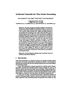
approaches such as Bayesian or regularisation techniques have been successfully used in the past to promote sparsity and condition the model learning. Those most relevant to our work are discussed in section 4. 2.2. Granger-causality Graphs Granger (1969) proposed a practical definition of causality in time series based on the accuracy of least-squares predictor functions. In brief, for two time series Z and Y , we say that Z Granger causes if, given all the other relevant information, a predictor function using the history of Z as input can forecast Y better (in the mean-square sense) than a function not using it. Similarly, a set of time series {Z1 , . . . , Zl } G-causes series Y if it can be predicted better using the past values of the set. The G-causal relationships can be described by a directed graph G = {V, E} (Eichler (2012)), where each node v ∈ V represents a time series in the system, and the directed edges represent the G-causal relationships between the series. In VARs the G-causality is captured within the W parameters matrix. When any of the parameters of the k-th task (k-th column of the W) referring to the p past values of the l-th input series is non-zero, we say that the l-th series G-causes series k, and we denote this in the G-causal graph by a directed edge el,k from vl to vk . w.,1 ↓ Fig. 1 shows a schema of the VAR parameters matrix W and the corresponding G-causal e 2,1 { graph for an example system of K = 7 series w with the number of lags p = 3. In 1(a) the gray cells are the non-zero elements, in 1(b) the circle nodes are the individual time series, the arrow edges are the G-causal links between the series1 . For example, the arrow from 2 to 1 indicates a) W matrix b) G-causal graph that series 2 G-causes series 1; correspondingly the cells for the 3 lags in the 2nd block-row and Figure 1: W and G-causal graph. e 2,1 ). Series 2 and the 1th column are shaded (w 5 are the leading indicators for the whole system, their block-rows are shaded in all columns in the W matrix schema and they have out-edges to all other nodes in the G-graph. One may question if calling the above notion causality is appropriate. Indeed, unlike other perhaps more philosophical approaches, e.g. Pearl (2009), it does not really seek to understand the underlying forces driving the relationships between the series. Instead, the concept is purely technical based on the series contribution to the predictive accuracy, ignoring also possible confounding effects of unobservables. Nevertheless, the term is well established in the time series community. Moreover, it fits very well our purposes, where the primary objective is to learn models with high forecast accuracy that use as inputs only those time series that contribute to improving the accuracy - the leading indicators. Therefore, acknowledging all the reservations, we stick to it in this paper always preceding it by Granger or G- to avoid confusion. 1. The self-loops corresponding to the block-diagonal elements in W are omitted for clarity of display.
4
Learning Predictive Leading Indicators
3. Learning VARs with Clusters around Leading Indicators We present here our new method for learning VAR models with task Clustering around Leading indicators (CLVAR). The method relies on the assumption that the generating process is sparse in the sense of there being only a few leading indicators within the system having an impact on the future developments. The leading indicators may be useful for predicting all or only some of the series in the systems. In this respect the series are clustered around their G-causing leading indicators. However, the method does not need to know the identity of the leading indicators nor the cluster assignments a priori and instead learns these together with the predictive models. In building our method we exploited the multi-task learning ideas (Caruana, 1997) and let the models benefit from learning multiple tasks together (one task per series). This is in stark contrast to other state-of-the-art VAR and graphical-Granger methods, e.g. Arnold et al. (2007); Lozano et al. (2009); Liu and Bahadori (2012). Albeit them being initially posed as multi-task (or multi-output) problems, due to their simple additive structure they decompose into a set of single-task problems solvable independently without any interaction and information sharing during the per-task learning. We, on the other hand, encourage the models to share information and borrow strength from one another in order to improve the overall performance by intertwining the model learning via structural constraints on the models derived from the assumptions outlined above. 3.1. Leading Indicators for Whole System For the sake of exposition we first concentrate on a simplified problem of learning a VAR with leading indicators shared by the whole system (without clustering). The structure we assume here is the one illustrated in Fig. 1. We see that the parameters matrix W is sparse with non-zero elements only in the block-rows corresponding to the lags of the leading indicators for the system (series 2 and 5 in the example in Fig. 1) and on the block diagonal. The block-diagonal elements of W are associated with the lags of each series serving as inputs for predicting its own 1-step-ahead future. It is a stylised fact that the future of a stationary time series depends first and foremost on its own past developments. Therefore in addition to the leading indicators we want each of the individual series forecast function to use its own past as a relevant input. We bring the above structural assumptions into the method by formulating novel fit-for-purpose constraints for learning VAR models with multi-task structured sparsity. 3.1.1. Learning Problem and Algorithm for Learning without Clusters We first introduce some new notation to accommodate for the necessary block structure across the lags of the input series in the input matrix X and the corresponding elements of the parameters matrix W. For each input vector xt,. (a row of X) we indicate by et,j = (yt−1,j , yt−2,j , . . . , yt−p,j )′ the p-long sub-vector of xt,. referring to the history (the p x lagged values preceding time t) of the series j, so that for the whole row we have xt,. = e′t,K )′ . Correspondingly, in each model vector w.,k (a column (xt,1 , . . . , xt,Kp )′ = (e x′t,1 , . . . , x e j,k the p-long sub-vector of the kth model parameters associated of W), we indicate by w e 2,1 is the block of the 3 shaded parameters in et,j . In Fig. 1, w with the input sub-vector x column 1 and rows {4, 5, 6} - the block of parameters of the model for forecasting the 1st 5
´ Kalousis Marchand-Maillet Gregorova
time series associated with the 3 lags of the 2nd time series (a leading indicator) as inputs. et,j and parameters w e j,k we can rewrite the inner products in Using these blocks of inputs x PK e b,k , x et,b i. the loss in (1) as hw.,k , xt,. i = b=1 hw Next, we associate each of the parameter blocks with a single non-negative scalar γb,k so e b,k = γb,k v eb,k . The Kp × K matrix V, composed of the blocks v eb,k in the same way that w e b,k , is therefore just a rescaling of the original W with the weights as W is composed of w γb,k used for each block. With this new re-parametrization the squared-error loss (1) is L(W) =
T X K K X X et,b i)2 . (yt,k − γb,k he vb,k , x t=1 k=1
(2)
b=1
Finally, we use the non-negative K × K weight matrix Γ = {γb,k | b, k = 1, . . . , K} to formulate our multi-task structured sparsity constraints. In Γ each element corresponds to a single series serving as an input to a single predictive model. A zero weight γb,k = 0 results e b,k = 0 and therefore the corresponding input sub-vectors in a zero parameter sub-vector w et,b (the past lags of series b for each time point t) have no effect in the predictive functions x for task k. Our assumption of only small number of leading indicators means that most series shall have no predictive effect for any of the tasks. This can be achieved by Γ having most of its rows equal to zero. On the other hand, the non-zero elements corresponding to the leading indicators shall form full rows of Γ. As explained in section 3.1, in addition to the leading indicators we also want each series past to serve as an input to its own forecast function. This translates to non-zero diagonal elements γi,i 6= 0. To combine these two contradicting structural requirements onto Γ (sparse rows vs. non-zero diagonal) we construct the matrix from two same size matrices Γ = A+B, one for each of the structures: A for the row-sparse of leading indicators, B for the diagonal of the own history. We now formulate the optimisation problem for learning VAR with shared leading indicators across the whole system and dependency on own past as the constrained minimisation PT PK PK et,j i)2 + λ||V||2F argminA,V vb,k , x (3) t=1 k=1 (yt,k − b=1 (αb,k + βb,k )he s.t.
1′K α = κ; α ≥ 0; α.,j = α, βj,j = 1 − αj,j ∀j = 1, . . . , K
,
where the links between the matrices A, B, Γ, V and the parameter matrix W of the VAR model are explained in the paragraphs above. In (3) we force all the columns of A to be equal to the same vector α2 , and we promote the sparsity in this vector by constraining it onto a simplex of size κ. κ controls the relative weight of each series own past vs. the past of all the neighbouring series. For identifiability reasons we force the diagonal elements of Γ to equal unity by scaling appropriately the diagonal βj,j elements. Lastly, while Γ is constructed and constrained to control for the structure of the learned models (as per our assumptions), the actual value of the final parameters W is the result of combining it with the other learned matrix V. To confine the overall complexity of the final model W we impose a standard ridge penalty (Hoerl and Kennard, 1970) on the model parameters V. 2. This does not excessively limit the capacity of the models as the final model matrix W is the result of combining Γ with the learned matrix V.
6
Learning Predictive Leading Indicators
The optimisation problem (3) is jointly non-convex, however, it is convex with respect to each of the optimisation variables with the other variable fixed. Therefore we propose to solve it by an alternating descent for A and V as outlined in algorithm 1 below. B is solved trivially applying directly the equality constraint of (3) over the learned matrix A as B = I − diag(A) which implies Γ = A + B = A − diag(A) + I. Algorithm 1: Alternating descent for VAR with system-shared leading indicators Input : training data Y, X; hyper-parameters λ, κ Initialise: α evenly to satisfy constraints in all columns of A; Γ ← A − diag(A) + I repeat // Alternating descent begin Step 1: Solve for V foreach task k do (k) et,b ∀ time point t and input series b re-weight input blocks zt,b ← γb,k x (k) 2 v.,k ← argminv ||y .,k − Z v||2 + λ||v||22 // standard ridge regression end end begin Step 2: Solve for A and Γ foreach task k do (k) et,b i ∀ time point t and input series b vb,k , x input products ht,b ← he (k)
task residuals after using own history rt,k ← yt,k − ht,k
∀ time point t
(k) ht,k
← 0 ∀ time point t remove own history from input products end concatenate vertically input product matrices H = vertcat(H(.) ) α ← argminα ||vec(R) − H α||22 , s.t. α on simplex // projected grad descent put α to all columns of A; Γ ← A − diag(A) + I end until objective convergence; To foster the intuition behind our method we provide links to other well-known learning problems and methods. First, we can rewrite the weighted inner product in the loss function et,b i. In this “feature learning” formulation the weights γb,k act on the (2) as he vb,k , γb,k x (k) et,b . These are original inputs and, hence, generate new task-specific features zt,b = γb,k x the ridge penalty actually used in Step 1 of our algorithm P we 2can express P 1. Alternatively, e b,k ||22 . In this “adaptive on V used in eq. (3) as ||V||2F = b,k ||e ||w vb,k ||22 = b,k 1/γb,k ridge” formulation the elements of Γ, which in our methods we learn, act as weights for the ℓ2 regularization of W. Equivalently, we can see this as the Bayesian maximum-a-posteriori with Guassian priors where the elements of Γ are the learned priors for the variance of the model parameters or (perhaps more interestingly) the random errors. 3.2. Leading Indicators for Clusters of Predictive Tasks After explaining in section 3.1 the simplified case of learning a VAR with leading indicators for the whole system, we now move onto the more complex (and for larger VARs certainly 7
´ Kalousis Marchand-Maillet Gregorova
more realistic) setting of the leading indicators being predictive only for parts of the system - clusters of predictive tasks. To get started we briefly consider the situation in which the cluster structure (not the leading indicators) is known a priori. Here the models could be learned by a simple modification of algorithm 1 where in step 2 we would work with cluster-specific vectors α and matrices H and R constructed over the known cluster members. In reality the clusters are typically not known and therefore our CLVAR method is designed to learn them together with the leading indicators. We use the same block decompositions of the input and parameter matrices X and W, and the structural matrices Γ = A+B = A−diag(A)+I and the rescaled parameter matrix V defined in section 3.1. However, we need to alter the structural assumptions encoded into the matrix A. In the cluster case A still shall have many rows equal to zero but it shall no longer have all the columns equal (same leading indicators for all the tasks). Instead, we learn it as a low rank matrix by factorizing it into two lower dimensional matrices A = DG: the K × r dictionary matrix D with the dictionary atoms (columns of D) representing the cluster prototypes of the dependency structure; and the r × K matrix G with the elements being the per-model dictionary weights, 1 ≤ r ≤ K. To better understand the clustering effect of the low-rank decomposition, Fig. 2 illustrates it for an imaginary system of K = 7 time series with rank r = 3. The d.,j j={1,2,3} columns in the top are the sparse cluster prototypes (the non-zero elements for the leading indicators are shaded). The (a) hard cluster (b) soft cluster ascircles in the bottom are the individual assignments signments learning tasks and the arrows are the permodel dictionary weights gi,j . Solid arrows Figure 2: Roles of D and G matrices in the low-rank decomposition A have weight 1, missing arrows have weight zero, dashed arrows have weight between 0 and 1. So for example, the solid arrow from the 2nd column to the 7th circle in Fig. 2(a) is the g2,7 element of matrix G. Since it is a full arrow, it is equal to 1. The arrow from the 3rd column to the 2nd circle in Fig. 2(b) is the g3,2 element of G. Since the arrow is dashed, we have 0 < g3,2 < 1. Fig. 2(a) uses a binary matrix G (no dashed arrows) reflecting hard clustering of the tasks consistent with our initial setting of a priori known clusters. Each task (circle at the bottom) is associated with only one cluster prototype (columns of D in the top). In contrast, Fig. 2(b) uses matrix G with elements between 0 and 1 to perform soft clustering of the tasks. Each task (circle at the bottom) may be associated with more than one cluster prototype (columns of D in the top). Our CLVAR is based on this latter approach of soft-clustering of the forecast tasks.
8
Learning Predictive Leading Indicators
3.2.1. Learning Problem and Algorithm for CLVAR We now adapt the minimisation problem (3) for the multi-cluster setting PT PK PK PK e′t,j i)2 + λ||V||2F (4) argminD,G,V v ′b,k , x t=1 k=1 (yt,k − b=1 ( j=1 db,j gj,k + βb,k )he s.t. 1′K d.,j = κ; d.,j ≥ 0; 1′r g.,j = 1; g.,j ≥ 0, βj,j = 1 − αj,j ∀j .
The relations of the optimisation matrices D, G, V to the parameter matrix W of the VAR model are as explained in the paragraphs above. The principal difference of the formulation (4) as compared to problem (3) is the low-rank decomposition of matrix A = DG using P the fact that ab,k = K d j=1 b,j gj,k . Similarly as for the single column α in (3) we promote sparsity in the cluster prototypes d.,j by constraining them onto the simplex. And we use the probability simplex constraints to sparsify the per-task weights in the columns of G so that the task are not based on all the prototypes. Algorithm 2: CLVAR - VAR with leading indicators for clusters of predictive tasks Input : training data Y, X; hyper-parameters λ, κ, r Initialise: D, G evenly to satisfy the constraints; A ← DG; Γ ← A − diag(A) + I repeat // Alternating descent begin Step 1: Solve for V same as in algorithm 1 end begin Step 2: Solve for D, G and Γ foreach task k do same as in algorithm 1 // projected grad desc g.,k ← argming ||r.,k − H(k) g||22 , s.t. g on simplex end concatenate vertically input product matrices H = vertcat(H(.) ) b ← G′ ⊗ 1T 1′ ; H b = 1′r ⊗ H expand matrices to match dictionary vectorization G K 2 b ⊙H b vec(D)|| // projected grad desc vec(D) ← argminD ||vec(R) − G 2 s.t. d.,j on simplex ∀j A = DG; Γ ← A − diag(A) + I end until objective convergence; We propose to solve problem (4) by alternating descent algorithm 2. While non-convex, the alternating approach for learning the low-rank matrix decomposition is known to perform well in practice and has been recently supported by new theoretical guarantees, e.g. Park et al. (2016). We solve the two sub-problems in step 2 by projected gradient descent with FISTA backtracking line search (Beck and Teboulle, 2009). The algorithm is O(T ) for increasing number of observation and O(K 3 ) for increasing number of time series. However, one needs to bear in mind that with each additional series the complexity of the VAR model itself increases by O(K). Nevertheless, the expensive scaling with K is an important bottleneck of our method and we are investigating options to address it in our future work.
9
´ Kalousis Marchand-Maillet Gregorova
4. Related Work We explained in section 2.2 how our search for leading indicators links to the Granger causality discovery in VARs. As shows the list of references in the survey of Liu and Bahadori (2012), this has been a rather active research area over the last several years. While the traditional approach for G-discovery was based on pairwise testing of candidate models or the use of model selection criteria such as AIC or BIC, inefficiency of such approaches for builidng predictive models of large time series system has long been recognised3 , e.g. Doan et al. (1984). As an alternative, variants of so-called graphical Granger methods based on regularization for parameter shrinkage and thresholding (along the lines of Lasso (Tibshirani, 2007)) have been proposed in the literature. We use the two best-established ones, the lasso-Granger (VARL1) of Arnold et al. (2007) and the grouped-lasso-Granger (VARLG) of Lozano et al. (2009), as the state-of-the-art competitors in our experiments. More recent adaptations of the graphical Granger method address the specific problems of determining the order of the models and the G-causality simultaneously (Shojaie and Michailidis, 2010; Ren et al., 2013), the G-causality inference in irregular (Bahadori and Liu, 2012) and subsampled series (Gong et al., 2015), and in systems with instantaneous effects (Peters et al., 2013). However, neither of the above methods considers or exploits any common structures in the G-causality graphs as we do in our method. Common structures in the dependency are assumed by Jalali and Sanghavi (2012) and Geiger et al. (2015) though the common interactions are with unobserved variables from outside the system rather then within the system itself. Also, the methods discussed in these have no clustering ability. Songsiri (2015) considers common structures across several datasets (in panel data setting) instead of within the dynamic dependencies of a single dataset. Huang and Schneider (2012) assume sparse bi-clustering of the G-graph nodes (by the in- and out- edges) to learn fully connected sub-graphs in contrast to our shared sparse structures. Most recently, Hong et al. (2017) proposes to learn clusters of series by Laplacian clustering over the sparse model parameters. However, the underlying models are treated independently not encouraging any common structures at learning. More broadly, our work builds on the multi-task (Caruana, 1997) and structured sparsity (Bach et al., 2012) learning techniques developed outside the time-series settings. Similar block-decompositions of the feature and parameter matrices as we use in our methods have been proposed to promote group structures across multiple models (Argyriou et al., 2007; Swirszcz and Lozano, 2012). Although the methods developed therein have no clustering capability. Various approaches for learning model clusters are discussed in Bakker and Heskes (2003); Xue et al. (2007); Jacob et al. (2009); Kang et al. (2011); Kumar and Hal Daume III (2012) of which the latest uses similar low-rank decomposition approach as our method. Nevertheless, neither of these approaches learns sparse models and builds the clustering on similar structural assumptions as our method does. 3. Due to the lack of domain knowledge to support the model selection and combinatorial complexity of exhaustive search.
10
Learning Predictive Leading Indicators
5. Experiments We present here the results of a set of experiments on synthetic and real-world datasets. We compare to relevant baseline methods for VAR learning: univariate auto-regressive model AR (though simple, AR is typically hard to beat by high-dimensional VARs when the domain knowledge cannot help to specify a relevant feature subset for the VAR model), VAR model with standard ℓ2 regularisation VARL2 (controls over-parametrisation by shrinkage but does not yield sparse models), VAR model with ℓ1 regularisation VARL1 (lasso-Granger of Arnold et al. (2007)), and VAR with group lasso regularisation VARLG (grouped-lassoGranger of Lozano et al. (2009)). We implemented all the methods in Matlab using standard state-of-the-art approaches: trivial analytical solutions for AR and VARL2, FISTA proximal-gradient (Beck and Teboulle, 2009) for VARL1 and VARLG. The full code together with the datasets amenable for full replication of our experiments is available from https://bitbucket.org/dmmlgeneva/var-leading-indicators. In all our experiments we simulated real-life forecasting exercises. We split the analysed datasets into training and hold-out sets unseen at learning and only used for performance evaluation. The trained models were used to produce one-step ahead forecasts by sliding through all the points in the hold-out. We repeated each experiments over 20 random re-samples. The reported performance is the averages over these 20 re-samples. The construction of the re-samples for the synthetic and real datasets is explained in the respective sections below. We used 3-folds cross-validation with mean squared error as the criterion for the hyper-parameter grid search. Unless otherwise stated below, the grids were: λ ∈ 15-elements grid [10−4 . . . 103 ] (used also for VARL2, VARL1 and VARLG), κ ∈ {0.5, 1, 2}, rank ∈ {1, 0.1K, 0.2K, K}. We preprocessed all the data by zero-centering and unit-standardization based on the training statistics only. For all the experiments and all the tested methods we fixed the lag of the learned models to p = 5. While the search for the best lag p has in the past constituted an important part of time series modelling4 , in high-dimensional settings the exhaustive search through possible sub-set model combinations is clearly impractical. Modern methods therefore focus on using VARs with sufficient number of lags to cater for the underlying time dependency and apply Bayesian or regularization methods to control the model complexity, e.g. Koop (2013). In our case, this is achieved by the ridge shrinkage on the parameter matrix V. 5.1. Synthetic Experiments We designed six generating processes for systems varying by number of series and the Gcausal structure. The first three are small systems with K = 10 series only, the next three increase the size to K = {30, 50, 100}. Systems 1 and 2 are unfavourable for our method, generated by processes not corresponding to our structural assumptions: in the 1st each series is generated from its own past only and therefore can be best modelled by a simple univariate AR model (the G-causal graph has no links); the 2nd is a fully connected VAR (all series are leading for the whole system). The 3rd system consists of 2 clusters with 5 series each, both depending on 1 leading indicator. Systems 4-6 are composed of {3, 5, 10} clusters respectively, each with 10 series concentrated around 2 leading indicators5 . 4. Especially for univariate models within the context of the more general ARMA class (Box et al., 1994). 5. For the last two, we fixed the rank in CLVAR training to the true number of clusters.
11
´ Kalousis Marchand-Maillet Gregorova
For each of the 6 system designs we first generated a random matrix of VAR coefficients with the required structure. We ensured the processes are stationary by controlling the roots of the model characteristic polynomials. We then generated 20 random realisation of the VAR processes with uncorrelated standard-normal noise. In each, we separated the last 500 observations into a hold-out set and used the previous T observations for training. Once trained, the same model was used for the 1-step-ahead forecasting of the 500 hold-out points by sliding forward through the dataset. The predictive performance of the methods in the 6 experimental settings for multiple training sizes T is summarised in Fig. 3(a)6 . We measure the predictive accuracy by the mean square error of 1-step-ahead forecasts relative to the forecasts produced by the VAR with the true generative coefficients (RelMSE). Doing so we standardize the MSE by the irreducible error of each of the forecast exercises. The closer to 1 (the gold standard) the better. The plots display the average RelMSE over the twenty replications of the experiments, the error bars are at ±1 standard deviation. In all the experiments the predictive performance improves with the increasing training size and the differences between the methods diminish. CLVAR outperforms all the other methods in the experiments with sparse structures as per our assumptions (mostly markedly). But CLVAR behaves well even in the unfavourable conditions of the first two systems. It still performs better than the other two sparse methods VARL1 and VARLG and the non-sparse VARL2 in the 1st completely sparse experiment7 , and it is on par with the other methods in the 2nd full VAR experiment. Ts=10, Clusters=1, Leading=0
1.8
15
1.6
1.6 10
1.4
1.4 5
1.2 1 50 2
RelMSE
0.5
70
90
110 130 150
50
Ts=30, Clusters=3, Leading=6
1.2
70
90
1 110 130 150 50
90
110 130 150
Ts=50, Clusters=5, Leading=10 Ts=100, Clusters=10, Leading=20 2 2
1.8
1.8
1.8
1.6
1.6
1.6
1.4
1.4
1.4
1.2
1.2
1.2
1 130 150 200 300 400 500 trainSize
AR
70
VARL2
VARLG
0.4
0.4
0.3
0.3
0.3
0.2
0.2
0.2
0.1
0.1
0.1
70
90
(a) Relative MSE over true model
110
130
0 50
150
Ts=30, Clusters=3, Leading=6
70
90
110
130
150
0 50
0.4
0.4
0.3
0.3
0.3
0.2
0.2
0.2
0.1
0.1
0.1
0 130
150
200 300 trainSize
400
70
90
110
130
150
Ts=50, Clusters=5, Leading=10 Ts=100, Clusters=10, Leading=20 0.5 0.5
0.4
AR
CLVAR
Ts=10, Clusters=1, Leading=10 Ts=10, Clusters=2, Leading=2 0.5 0.5
0.4
0.5
1 1 130 150 200 300 400 500 130 200 400 600 800 1000 trainSize trainSize
VARL1
Ts=10, Clusters=1, Leading=0
0 50
selection error
RelMSE
1.8
Ts=10, Clusters=1, Leading=10 Ts=10, Clusters=2, Leading=2 20 2
selection error
2
500
VARL2
0 130
150
200 300 trainSize
VARL1
400
0 500 130
VARLG
200
400 600 trainSize
800 1000
CLVAR
(b) Selection error of G-causal links
Figure 3: Results for synthetic experiments averaged over 20 experimental replications In Fig. 3(b) we show the accuracy of the methods in selecting the true generative Gcausal links between the series in the system. The selection error (the lower the better) is measured as the average of the false negative and false positive rates. We plot the averages with ±1 standard deviation over the 20 experimental replications. The CLVAR typically learned models structurally closer to the true generating process than the other tested methods, in most cases with substantial advantage. 6. Numerical results behind the plots are listed in the Supplement. 7. The AR model is in an advantage here since it has the true-process structure by construction.
12
Learning Predictive Leading Indicators
Ts=30, Clusters=3, Leading=6
To better understand the behaviour of TRUE VARL1 VARLG CLVAR the methods in terms of the structure they learn, we chart in Fig. 4 a synthesis of the model matrices W learned by the sparse learning methods for the largest training size in the 4th system8 . The displayed Figure 4: Synthesis of model parameters W structures correspond to the schema of the W matrix presented in Fig.1. For the figure, the matrices were binarised to simply indicate the existence (1) or non-existence (0) of a G-causal link. The white-to-black shading reflects the number of experimental replications in which this binary indicator is active (equal to 1). So, a black element in the matrix means that this G-causal link was learned in all the 20 re-samples of the generating process. White means no G-causality in any of the re-samples. Though none of the sparse method was able to clearly and systematically recover the true structures, VARL1 and VARLG clearly suffer from more numerous and more frequent over-selections than CLVAR which matches the true structure more closely and with higher selection stability (fewer light-shaded elements). Finally, we explored how the CLVAR scales with increasing sample size T and the number of time series K. The empirical results correspond to the complexity analysis of section 3.2: the run-times increased fairly slowly with increasing sample size T but were much longer for systems with higher number of series K. Further details are deferred to the Supplement. Overall, the synthetic experiments confirm the desired properties of CLVAR in terms of improved predictive accuracy and structural recovery. 20
20
15
15
10
10 5
5.2. Real-data Experiments We used two real datasets very different in nature, frequency and length of available observations. First, an USGS dataset of daily averages of water physical discharge9 measured at 17 sites along the Yellowstone (8 sites) and Connecticut (9 sites) river streams (source: Water Services of the US geological survey http://www.usgs.gov/). Second, an economic dataset of quarterly data on 20 major US macro-economic indicators of Stock and Watson (2012) frequently used as a benchmark dataset for VAR learning methods. More details on the datasets can be found in the Supplement. We preprocessed the data by standard stationary transformations: we followed Stock and Watson (2012) for the economic dataset; by year-on-year log-differences for the USGS. For the short economic dataset, we fixed the hold-out length to 30 and the training sizes from 50 to 130. For the much longer USGS dataset, the hold-out is 300 and the training size increases from 200 to 600. The re-samples are constructed by dropping the latest observation from the data and constructing the shifted train and hold-out from this curtailed dataset. The results of the two sets of experiments are presented in Fig. 5. The true parameters of the generative processes are unknown here. Therefore the predictive accuracy is measured in terms of the MSE relative to a random walk model (the lower the better), and the structural recovery is measured in terms of the proportion of active edges in the G-causal 8. For space reasons, results for the other experiments are deferred to the Supplement. 9. USGS parameter code 00060 - physical discharge in cubic feet per second.
13
´ Kalousis Marchand-Maillet Gregorova
Economic Ts=20
0.6
1
Economic Ts=20
Economic Ts=20
0.5
edges
RelMSE
VARL1
0.4
VARLG
CLVAR
0.5
20 15 10
0.3
50
70 90 110 USGS Ts=17
1.4
0 50
130
1
70 90 110 USGS Ts=17
5
130
edges
RelMSE
USGS Ts=17 1.2 1
VARL1
VARLG
CLVAR
20
0.5 15
0.8 0.6 200
300
400 500 trainSize
AR
VARL2
600 VARL1
0 200
10
300 VARLG
400 500 trainSize
600 5
CLVAR
(b) Synthesis of parameters W
(a) MSE and G-causal edges
Figure 5: Results for real-data experiments averaged over 20 experimental replications graph (the lower the better), always averaged across the 20 re-samples with ±1 standard deviation errorbar. Similarly as in the synthetic experiments, the predictive performance improves with increasing training size and the differences between the methods get smaller. In both experiments, the non-sparse VARL2 has the worst forecasting accuracy (which corresponds to the initial motivation that real large time-series systems tend to be sparse). CLVAR outperformed the other two sparse learning methods VARL1 and VARLG in predictive accuracy as well as sparsity of the learned G-causal graphs. In the economic experiment, the completely (by construction) sparse AR achieved similar predictive accuracy. CLVAR clearly outperforms all the other methods on the USGS dataset. Fig. 5(b) explores the effect of the structural assumptions on the final shape of the model parameter matrices W in the same manner as in Fig. 4. The CLVAR matrices are much sparser than the VARL1 and VARLG matrices, organised around a small number of leading indicators. In the economic dataset, the CLVAR method identified three leading indicators for the whole system. In the USGS dataset, the dashed red lines delimit the the Yellowstone (top-left) from the Connecticut (bottom-right) sites. In both these sets of experiments the recovered structure helped improving the forecasts beyond the accuracy achievable by the other tested learning methods.
6. Conclusions We presented here a new method for learning sparse VAR models with shared structures in their Granger causality graphs based on the leading indicators of the system, a problem that had not been previously addressed in the time series literature. The new method has multiple learning objectives: good forecasting performance of the models, and the discovery of the leading indicators and the clusters of series around them. Meeting these simultaneously is not trivial and we used the techniques of multi-task and structured sparsity learning to achieve it. The method promotes shared patterns in the structure of the individual predictive tasks by forcing them onto a lower-dimensional sub-space spanned by sparse prototypes of the cluster centres. The empirical evaluation confirmed the efficacy of our approach through favourable results of our new method as compared to the state-of-the-art. 14
Learning Predictive Leading Indicators
References A. Argyriou, T. Evgeniou, and M. Pontil. Multi-task feature learning. NIPS, 2007. Andrew Arnold, Yan Liu, and Naoki Abe. Temporal causal modeling with graphical granger methods. Proceedings of the 13th ACM SIGKDD - KDD ’07, 2007. Francis Bach, Rodolphe Jenatton, Julien Mairal, and Guillaume Obozinski. Structured Sparsity through Convex Optimization. Statistical Science, 2012. Mohammad Taha Bahadori and Yan Liu. On Causality Inference in Time Series. 2012 AAAI Fall Symposium Series, 2012. Bart Bakker and Tom Heskes. Task clustering and gating for bayesian multitask learning. Journal of Machine Learning Research, 2003. Amir Beck and Marc Teboulle. Gradient-based algorithms with applications to signal recovery. Convex Optimization in Signal Processing and Communications, 2009. George E. P. Box, Gwilym M. Jenkins, and Gregory C. Reinsel. Time Series Analysis: Forecasting and Control. Prentice-Hall International, Inc., 3rd edition, 1994. Rich Caruana. Multitask Learning. PhD thesis, Carnegio Mellon University, 1997. Thomas Doan, Robert Litterman, and Christopher Sims. Forecasting and conditional projection using realistic prior distributions. Econometric reviews, 3(1):1–100, 1984. Michael Eichler. Graphical modelling of multivariate time series. Probability Theory and Related Fields, 2012. Theodoros Evgeniou and Massimiliano Pontil. Regularized multi–task learning. Proceedings of the 10th ACM SIGKDD, 2004. P. Geiger, K. Zhang, M. Gong, D. Janzing, and B. Sch¨ olkopf. Causal Inference by Identification of Vector Autoregressive Processes with Hidden Components. ICML, 2015. Mingming Gong, Kun Zhang, Dacheng Tao, Philipp Geiger, and Intelligent Systems. Discovering Temporal Causal Relations from Subsampled Data. In ICML, 2015. CWJ W J Granger. Investigating Causal Relations by Econometric Models and Crossspectral Methods. Econometrica: Journal of the Econometric Society, 1969. Arthur E. Hoerl and Robert W. Kennard. Ridge regression: biased estimation for nonorthogonal problems. Technometrics, 1970. Dezhi Hong, Quanquan Gu, and Kamin Whitehouse. High-dimensional Time Series Clustering via Cross-Predictability. AISTATS, 2017. TK Huang and Jeff Schneider. Learning bi-clustered vector autoregressive models. 2012. Laurent Jacob, Francis Bach, and JP P Vert. Clustered multi-task learning: A convex formulation. In Advances in Neural Information Processing Systems (NIPS), 2009. 15
´ Kalousis Marchand-Maillet Gregorova
Ali Jalali and Sujay Sanghavi. Learning the dependence graph of time series with latent factors. In International Conference on Machine Learning (ICML), 2012. Zhuoliang Kang, Kristen Grauman, and Fei Sha. Learning with Whom to Share in Multitask Feature Learning. In ICML, 2011. Gary Koop. Forecasting with medium and large Bayesian VARs. Journal of Applied Econometrics, 203(28):177–203, 2013. Abhishek Kumar and Hal Daume III. Learning task grouping and overlap in multi-task learning. In International Conference on Machine Learning (ICML), 2012. Yan Liu and MT Bahadori. A Survey on Granger Causality: A Computational View. Technical report, University of Southern California, 2012. Aur´elie C. Lozano, Naoki Abe, Yan Liu, and Saharon Rosset. Grouped graphical Granger modeling for gene expression regulatory networks discovery. Bioinformatics, 2009. Helmut L¨ utkepohl. New introduction to multiple time series analysis. Springer, 2005. D. Park, A. Kyrillidis, C. Caramanis, and S. Sanghavi. Finding low-rank solutions to smooth convex problems via the Burer-Monteiro approach. In Allerton Conference on Communication, Control, and Computing, 2016. Judea Pearl. Causality. Cambridge University Press, 2009. Jonas Peters, Dominik Janzing, and Bernhard Sch¨ olkopf. Causal Inference on Time Series using Restricted Structural Equation Models. In NIPS, 2013. Yunwen Ren, Zhiguo Xiao, and Xinsheng Zhang. Two-step adaptive model selection for vector autoregressive processes. Journal of Multivariate Analysis, 2013. Ali Shojaie and George Michailidis. Discovering graphical Granger causality using the truncating lasso penalty. Bioinformatics (Oxford, England), 2010. Jitkomut Songsiri. Sparse autoregressive model estimation for learning Granger causality in time series. In Proceedings of the 38th ICASSP, 2013. Jitkomut Songsiri. Learning Multiple Granger Graphical Models via Group Fused Lasso. In IEEE Asian Control Conference (ASCC), 2015. James H. Stock and Mark W. Watson. Generalized Shrinkage Methods for Forecasting Using Many Predictors. Journal of Business & Economic Statistics, 2012. Grzegorz Swirszcz and Aurelie C Lozano. Multi-level Lasso for sparse multi-task regression. In International Conference on Machine Learning (ICML), 2012. Robert Tibshirani. Regression Shrinkage and Selection via the Lasso. Journal of the Royal Statistical Society. Series B: Statistical Methodology, 2007. Ya Xue, Xuejun Liao, Lawrence Carin, and Balaji Krishnapuram. Multi-task learning for classification with Dirichlet process priors. Journal of Machine Learning Research, 2007.
16
Learning Predictive Leading Indicators
Appendix A. Experimental data and transformations Table 1 lists the measurement sites of the Water Service of the US Geological Survey (http://www.usgs.gov/) whose data we use in the USGS experiments in section 5.2 of the main text. The original data are the daily averages of the physical discharge in cubic feet per second (parameter code 00060) downloaded from the USGS database on 9/9/2016. We have used the data up to 31/12/2014 and before modelling transformed them by taking the year-on-year log-differences. Table 1: Measurement sites for the river-flow data Code 06191500 06192500 06214500 06295000 06309000 06327500 06329500 01129200 01129500 01131500 01138500 01144500 01154500 01170500 01184000
Description Yellowstone River at Corwin Springs MT Yellowstone River near Livingston MT Yellowstone River at Billings MT Yellowstone River at Forsyth MT Yellowstone River at Miles City MT Yellowstone River at Glendive MT Yellowstone River near Sidney MT CONNECTICUT R BELOW INDIAN STREAM NR PITTSBURG, NH CONNECTICUT RIVER AT NORTH STRATFORD, NH CONNECTICUT RIVER NEAR DALTON, NH CONNECTICUT RIVER AT WELLS RIVER, VT CONNECTICUT RIVER AT WEST LEBANON, NH CONNECTICUT RIVER AT NORTH WALPOLE, NH CONNECTICUT RIVER AT MONTAGUE CITY, MA CONNECTICUT RIVER AT THOMPSONVILLE, CT
Table 3 lists the macro-economic indicators of Stock and Watson (2012) used in our economic experiment in section 5.2 in the main text. Before using for modelling we have applied the same pre-processing steps as in Stock and Watson (2012). We have • transformed the monthly data to quarterly by taking the quarterly averages (column Q in table 3); • applied the stationarizing transformations described in table 2 (column T in table 3); • cleaned the data from outliers by replacing observations with absolute deviations from median larger than 6 times the interquartile range by the median of the 5 preceding values.
Appendix B. Experimental results This section provides further details on experimental results not included in the main text due to space limitation.
17
´ Kalousis Marchand-Maillet Gregorova
Table 2: Stationarizing transformations T 1 2 3 4 5 6
Transformation yt = zt yt = zt − zt−1 yt = (zt − zt−1 ) − (zt−1 − zt−2 ) yt = log(zt ) yt = ln(zt /zt−1 ) yt = ln(zt /zt−1 ) − ln(zt−1 /zt−2 )
zt is the original data, yt is the transformed series
Table 3: Macro-economic data and transformations Code GDP251 CPIAUCSL FYFF PSCCOMR FMRNBA FMRRA FM2 GDP252 IPS10 UTL11 LHUR HSFR PWFSA GDP273 CES275R FM1 FSPIN FYGT10 EXRUS CES002
Q Q M M M M M M Q M M M M M Q M M M M M M
T 5 6 2 5 3 6 6 5 5 1 2 4 6 6 5 6 5 2 5 5
Description real gross domestic product, quantity index (2000=100) , saar cpi all items (sa) fred interest rate: federal funds (effective) (% per annum,nsa) real spot mrkt price idx:bls & crb: all commod(1967=100) depository inst reserves:nonborrowed,adj res req chgs(mil$ ,sa) depository inst reserves:total,adj for reserve req chgs(mil$ ,sa) money stock:m2 (bil$,sa) real personal consumpt expend, quantity idx (2000=100) , saar industrial production index - total index capacity utilization - manufacturing (sic) unemployment rate: all workers, 16 years & over (% ,sa) housing starts:nonfarm(1947-58),total farm& nonfarm(1959-) producer price index: finished goods (82=100,sa) personal consumption expenditures, price idx (2000=100) , saar real avg hrly earnings, prod wrkrs, nonfarm - goods-producing money stock: m1(bil$ ,sa) s& p’s common stock price index: industrials (1941-43=10) interest rate: u.s.treasury const matur,10-yr.(% per ann,nsa) united states,effective exchange rate(merm)(index no.) employees, nonfarm - total private
B.1. Synthetic experiments Fig. 6 shows the synthesis of the model parameter matrices W for the six synthetic experimental designs. The displayed structures correspond to the schema of the W matrix presented in Fig. 1 of the main text. For the figure, the matrices were binarised to simply indicate the existence (1) or non-existence (0) of a G-causal link. The white-to-black shading reflects the number of experimental replications in which this binary indicator is active (equal to 1). So, a black element in the matrix means that this G-causal link was learned in all the 20 re-samples of the generating process. White means no G-causality in any of
18
Learning Predictive Leading Indicators
the re-samples. Though none of the sparse method was able to clearly and systematically recover the true structures, VARL1 and VARLG clearly suffer from more numerous and more frequent over-selections than CLVAR which matches the true structures more closely and with higher selection stability (fewer light-shaded elements). The 4th experimental set-up is included in the main text as Fig. 4. Ts=10, Clusters=1, Leading=0 TRUE
VARL1
VARLG
Ts=10, Clusters=1, Leading=10 CLVAR
20
TRUE
VARL1
VARLG
VARL1
VARLG
CLVAR
20 15
10
10
5
5
Ts=30, Clusters=3, Leading=6 CLVAR
20
TRUE
VARL1
VARLG
CLVAR
20
15
15
10
10
5
5
Ts=50, Clusters=5, Leading=10 TRUE
VARLG
15
Ts=10, Clusters=2, Leading=2 TRUE
VARL1
Ts=100, Clusters=10, Leading=20 CLVAR
20
TRUE
VARL1
VARLG
CLVAR
20
15
15
10
10
5
5
Figure 6: Synthesis of model parameters W Fig. 7 summarises the scaling properties of the CLVAR method with increasing increasing sample size T and the number of time series K. In each experiment, we selected a single hyper-parameter combination (near the optimal) and measured the time in seconds (on a single Intel(R) Xeon(R) CPU E5-2680 v2 @ 2.80GHz) and the number of iterations needed till the convergence of the objective (with 10−5 tolerance) for the 20 data re-samples. We used the ℓ2 regularised solution as a warm start. The empirical results correspond to the theoretical complexity analysis of section 3.2 in the main text. For an experimental set-up with fixed number of series K (and G-causal structure), the run-time typically grows fairly slowly with the sample sizes T . However, the increases are much more important when moving to larger experiments, with higher K and more complicated structures. Here the growth in run-time is accompanied by higher number of iterations. From our experimental set-up it is difficult to separate the effect of enlarging the time-series systems in terms of higher K from the effect of more complicated structures in terms of higher number of clusters and leading indicators. In reality, we expect these to go hand-in-hand so in this sense our empirical analysis complements the theoretical asymptotic complexity analysis of section 3.2 of the main text Table 4 provides the numerical data behind the plots of Fig. 3(a) in the main text. The predictive accuracy is measured by mean squared error (MSE) of 1-step-ahead forecasts relative to the forecasts produced by the VAR with the true generative coefficients (the 19
´ Kalousis Marchand-Maillet Gregorova
Ts=10, Clusters=1, Leading=10
time (s)
10
10 4
3
10 4 10
10 2
10 3 10 2
1
1
10
10 2
10 0 10 -1
50
70
90
110
130
150
10
10 1 10 -1
time (s)
10 4
3
10
10 3 10 2 1
10 2
10 0 200 300 trainSize
400
70
90
110
130
150
10 1
500
10
10 4 10 3 10 2
10 0
10 1 10 -1 130
150
200 300 trainSize
time
400
10 4
10 3
10 3
10 2 10
1
10 2
10 0 10 -1
50
70
90
110
130
150
10 1
Ts=100, Clusters=10, Leading=20
3
1
150
50
10 4
10 2
10 -1 130
10 2
10 4
Ts=50, Clusters=5, Leading=10
10 4
10
10 3
10 0
Ts=30, Clusters=3, Leading=6
10
10 4
3
numIter
10 4
Ts=10, Clusters=2, Leading=2
500
10 1
10 4
10 4
10 3 10 2 10
10 3
1
10 2
10 0 10 -1 130
numIter
Ts=10, Clusters=1, Leading=0
200
400 500 trainSize
800
10 1 1000
numIter
Figure 7: Runtime and number of iterations irreducible error). The relative MSE is averaged over the 500 hold-out points (the models are fixed and the forecasts are produced by sliding forward over the dataset). The avg and std are the average and standard deviation calculated over the 20 re-samples of the data for each experimental design. Table 4: Synthetic experiments: Relative MSE over true model trainSize 50 70 90 110 130 150
50
stat avg std avg std avg std avg std avg std avg std avg
AR
VARL2
VARL1
VARLG
Ts=10, Clusters=1, Leading=0 1.225 3.113 1.974 2.513 0.102 0.637 0.310 0.515 1.143 2.570 1.503 1.868 0.063 0.474 0.162 0.304 1.098 2.186 1.324 1.545 0.043 0.353 0.125 0.203 1.071 1.926 1.232 1.368 0.030 0.268 0.086 0.133 1.052 1.745 1.172 1.267 0.020 0.230 0.062 0.096 1.043 1.617 1.143 1.214 0.017 0.178 0.050 0.076 Ts=10, Clusters=1, Leading=10 12.564 23.449 42.347 42.055 continues in next 20
CLVAR 1.772 0.643 1.395 0.328 1.219 0.082 1.160 0.055 1.121 0.038 1.102 0.034 22.319 page ...
Learning Predictive Leading Indicators
trainSize 70 90 110 130 150
50 70 90 110 130 150
130 150 200 300 400 500
130 150
stat std avg std avg std avg std avg std avg std avg std avg std avg std avg std avg std avg std avg std avg std avg std avg std avg std avg std avg std avg std
... continues from previous page AR VARL2 VARL1 VARLG CLVAR 5.258 18.273 32.893 32.115 15.458 12.649 12.712 9.610 9.634 11.692 4.507 4.565 3.681 3.472 4.769 12.281 4.905 4.943 4.897 4.934 4.697 1.545 1.513 1.547 1.584 12.583 3.569 3.565 3.562 3.509 4.316 0.940 0.939 0.940 0.917 12.028 2.527 2.523 2.519 2.477 3.762 0.480 0.479 0.477 0.486 11.637 2.195 2.194 2.189 2.158 3.157 0.417 0.417 0.414 0.433 Ts=10, Clusters=2, Leading=2 1.429 2.730 1.743 2.124 1.674 0.167 0.565 0.246 0.357 0.308 1.336 2.296 1.522 1.689 1.405 0.096 0.346 0.206 0.199 0.139 1.295 1.998 1.398 1.499 1.289 0.100 0.253 0.139 0.146 0.116 1.258 1.824 1.320 1.396 1.199 0.064 0.214 0.082 0.103 0.062 1.237 1.686 1.283 1.347 1.156 0.057 0.181 0.078 0.085 0.050 1.229 1.566 1.255 1.300 1.133 0.054 0.171 0.076 0.081 0.043 Ts=30, Clusters=3, Leading=6 1.532 2.424 1.355 1.490 1.261 0.142 0.361 0.091 0.131 0.081 1.512 2.245 1.319 1.414 1.225 0.129 0.308 0.081 0.111 0.062 1.471 1.861 1.257 1.289 1.172 0.113 0.205 0.062 0.069 0.048 1.451 1.586 1.164 1.224 1.100 0.103 0.135 0.039 0.051 0.031 1.438 1.375 1.119 1.151 1.073 0.100 0.086 0.028 0.036 0.024 1.434 1.298 1.097 1.116 1.059 0.099 0.068 0.023 0.027 0.018 Ts=50, Clusters=5, Leading=10 3.327 4.376 2.024 2.160 1.746 0.557 0.792 0.306 0.277 0.223 3.254 3.920 1.801 1.915 1.577 0.544 0.685 0.205 0.215 0.196 continues in next page ... 21
´ Kalousis Marchand-Maillet Gregorova
trainSize 200 300 400 500
130 200 400 600 800 1000
... continues from previous page stat AR VARL2 VARL1 VARLG CLVAR avg 3.200 3.203 1.583 1.620 1.324 std 0.506 0.523 0.146 0.145 0.109 avg 3.161 2.280 1.347 1.392 1.128 std 0.491 0.301 0.083 0.092 0.034 avg 3.123 1.844 1.228 1.299 1.091 std 0.478 0.192 0.053 0.070 0.025 avg 3.097 1.622 1.172 1.214 1.081 std 0.468 0.144 0.039 0.050 0.025 Ts=100, Clusters=10, Leading=20 avg 1.890 3.362 1.518 1.807 1.734 std 0.202 0.536 0.118 0.184 0.178 avg 1.845 2.855 1.350 1.478 1.415 std 0.189 0.420 0.078 0.106 0.109 avg 1.801 2.196 1.225 1.268 1.180 std 0.177 0.264 0.050 0.059 0.049 avg 1.783 1.820 1.137 1.191 1.108 std 0.172 0.182 0.031 0.043 0.026 avg 1.777 1.644 1.104 1.129 1.084 std 0.170 0.142 0.023 0.029 0.021 avg 1.774 1.501 1.090 1.100 1.065 std 0.170 0.115 0.020 0.022 0.019
Table 5 provides the numerical data behind the plots of Fig. 3(b) in the main text. The selection accuracy of the true G-causal links is measured by the average between the false negative and false positive rates. The avg and std are the average and standard deviation calculated over the 20 re-samples of the data for each experimental design. Table 5: Synthetic experiments: Selection errors of true Gcausal links trainSize 50 70 90 110
stat avg std avg std avg std avg std
AR
VARL2
VARL1
VARLG
Ts=10, Clusters=1, Leading=0 0.000 0.500 0.268 0.316 0.000 0.000 0.062 0.072 0.000 0.500 0.245 0.318 0.000 0.000 0.027 0.056 0.000 0.500 0.207 0.301 0.000 0.000 0.027 0.026 0.000 0.500 0.172 0.285 0.000 0.000 0.026 0.027 continues in next 22
CLVAR 0.151 0.153 0.119 0.094 0.118 0.043 0.122 0.034 page ...
Learning Predictive Leading Indicators
trainSize 130 150
50 70 90 110 130 150
50 70 90 110 130 150
130 150 200 300 400 500
stat avg std avg std
AR 0.000 0.000 0.000 0.000
... continues from previous page VARL2 VARL1 VARLG CLVAR 0.500 0.141 0.268 0.138 0.000 0.017 0.029 0.036 0.500 0.120 0.245 0.143 0.000 0.019 0.027 0.041
Ts=10, Clusters=1, Leading=10 0.450 0.000 0.027 0.031 0.000 0.000 0.084 0.095 0.450 0.000 0.013 0.013 0.000 0.000 0.054 0.058 0.450 0.000 0.001 0.000 0.000 0.000 0.005 0.000 0.450 0.000 0.000 0.000 0.000 0.000 0.000 0.000 0.450 0.000 0.000 0.000 0.000 0.000 0.000 0.000 0.450 0.000 0.000 0.000 0.000 0.000 0.000 0.000 Ts=10, Clusters=2, Leading=2 avg 0.222 0.500 0.190 0.268 std 0.000 0.000 0.041 0.041 avg 0.222 0.500 0.179 0.248 std 0.000 0.000 0.072 0.039 avg 0.222 0.500 0.159 0.222 std 0.000 0.000 0.067 0.030 avg 0.222 0.500 0.155 0.200 std 0.000 0.000 0.086 0.031 avg 0.222 0.500 0.192 0.205 std 0.000 0.000 0.107 0.076 avg 0.222 0.500 0.210 0.196 std 0.000 0.000 0.118 0.064 Ts=30, Clusters=3, Leading=6 avg 0.321 0.500 0.175 0.204 std 0.000 0.000 0.015 0.017 avg 0.321 0.500 0.165 0.192 std 0.000 0.000 0.016 0.018 avg 0.321 0.500 0.178 0.183 std 0.000 0.000 0.046 0.014 avg 0.321 0.500 0.225 0.166 std 0.000 0.000 0.012 0.027 avg 0.321 0.500 0.202 0.242 std 0.000 0.000 0.013 0.012 avg 0.321 0.500 0.184 0.220 continues in next avg std avg std avg std avg std avg std avg std
23
0.043 0.112 0.010 0.026 0.017 0.042 0.000 0.000 0.000 0.000 0.000 0.000 0.168 0.103 0.096 0.061 0.094 0.051 0.058 0.044 0.067 0.054 0.054 0.034 0.173 0.037 0.176 0.027 0.165 0.029 0.107 0.034 0.098 0.029 0.095 page ...
´ Kalousis Marchand-Maillet Gregorova
trainSize
130 150 200 300 400 500
130 200 400 600 800 1000
... continues from previous page AR VARL2 VARL1 VARLG CLVAR 0.000 0.000 0.009 0.013 0.022 Ts=50, Clusters=5, Leading=10 avg 0.321 0.500 0.226 0.226 0.123 std 0.000 0.000 0.040 0.010 0.032 avg 0.321 0.500 0.211 0.217 0.110 std 0.000 0.000 0.039 0.011 0.035 avg 0.321 0.500 0.212 0.196 0.077 std 0.000 0.000 0.047 0.009 0.027 avg 0.321 0.500 0.257 0.169 0.038 std 0.000 0.000 0.011 0.021 0.008 avg 0.321 0.500 0.236 0.183 0.034 std 0.000 0.000 0.012 0.047 0.011 avg 0.321 0.500 0.224 0.218 0.033 std 0.000 0.000 0.011 0.033 0.011 Ts=100, Clusters=10, Leading=20 avg 0.321 0.500 0.120 0.164 0.260 std 0.000 0.000 0.006 0.009 0.054 avg 0.321 0.500 0.098 0.132 0.159 std 0.000 0.000 0.006 0.006 0.028 avg 0.321 0.500 0.158 0.094 0.121 std 0.000 0.000 0.006 0.006 0.016 avg 0.321 0.500 0.129 0.175 0.104 std 0.000 0.000 0.004 0.005 0.011 avg 0.321 0.500 0.110 0.154 0.100 std 0.000 0.000 0.004 0.005 0.011 avg 0.321 0.500 0.096 0.137 0.090 std 0.000 0.000 0.004 0.004 0.013
stat std
B.2. Real-data experiments Table 6 provides the numerical data behind the plots of Fig. 5(a) in the main text. The predictive accuracy is measured by mean squared error (MSE) of 1-step-ahead forecasts relative to the forecasts produced random walk model (= uses the last observed value as the 1-step-ahead forecast). The relative MSE is averaged over the 30 and 300 hold-out points for the Economic and the USGS dataset respectively (the models are fixed and the forecasts are produced by sliding forward over the dataset). The avg and std are the average and standard deviation calculated over the 20 re-samples of the data for each experimental dataset.
24
Learning Predictive Leading Indicators
Table 6: Real-data experiments: Relative MSE over random walk trainSize 50 70 90 110 130
200 300 400 500 600
stat avg std avg std avg std avg std avg std avg std avg std avg std avg std avg std
AR
VARL2
VARL1
Economic Ts=20 0.413 0.573 0.498 0.035 0.026 0.016 0.419 0.489 0.456 0.028 0.025 0.041 0.400 0.455 0.420 0.025 0.024 0.023 0.384 0.424 0.379 0.022 0.024 0.022 0.380 0.406 0.368 0.023 0.026 0.022 USGS Ts=17 0.912 1.857 1.222 0.013 0.098 0.058 0.881 1.320 0.876 0.003 0.040 0.012 0.858 0.934 0.760 0.001 0.030 0.026 0.855 0.855 0.754 0.003 0.021 0.011 0.862 0.858 0.747 0.002 0.004 0.004
VARLG
CLVAR
0.498 0.018 0.470 0.027 0.442 0.021 0.395 0.029 0.368 0.026
0.436 0.036 0.409 0.025 0.392 0.025 0.370 0.025 0.367 0.024
1.222 0.046 0.922 0.019 0.756 0.012 0.714 0.007 0.729 0.020
0.980 0.069 0.746 0.035 0.708 0.019 0.675 0.015 0.679 0.024
Table 7 provides the numerical data behind the plots of Fig. 5(b) in the main text. The sparsity of the learned models is measured by the proportion of active edges in the learned G-causality graph. The avg and std are the average and standard deviation calculated over the 20 re-samples of the data for each experimental dataset. Table 7: Real-data experiments: proportion of G-causal graph edges trainSize
stat
AR
50
avg std avg std
0.050 0.000 0.050 0.000
70
VARL2
VARL1
VARLG
Economic Ts=20 1.000 0.127 0.207 0.000 0.092 0.012 1.000 0.394 0.172 0.000 0.177 0.012 continues in next 25
CLVAR 0.115 0.024 0.110 0.026 page ...
´ Kalousis Marchand-Maillet Gregorova
trainSize 90 110 130
200 300 400 500 600
stat avg std avg std avg std
AR 0.050 0.000 0.050 0.000 0.050 0.000
avg std avg std avg std avg std avg std
0.059 0.000 0.059 0.000 0.059 0.000 0.059 0.000 0.059 0.000
... continues from previous page VARL2 VARL1 VARLG CLVAR 1.000 0.505 0.166 0.138 0.000 0.100 0.011 0.053 1.000 0.502 0.412 0.182 0.000 0.009 0.204 0.040 1.000 0.507 0.570 0.199 0.000 0.007 0.096 0.042 USGS Ts=17 1.000 0.618 0.465 0.363 0.000 0.117 0.061 0.057 1.000 0.581 0.641 0.369 0.000 0.018 0.010 0.081 1.000 0.629 0.625 0.412 0.000 0.143 0.005 0.060 1.000 0.823 0.640 0.431 0.000 0.061 0.009 0.057 1.000 0.801 0.632 0.450 0.000 0.014 0.090 0.020
26