Learning to Move Amid Uncertainty - CiteSeerX

Learning to Move Amid Uncertainty ROBERT A. SCHEIDT,1,2 JONATHAN B. DINGWELL,2 AND FERDINANDO A. MUSSA-IVALDI2 1 Department of Biomedical Engineering, Marquette University, Milwaukee, Wisconsin 53201; and 2Sensory Motor Performance Program, Rehabilitation Institute of Chicago, Chicago, Illinois 60611 Received 27 November 2000; accepted in final form 3 May 2001

Scheidt, Robert A., Jonathan B. Dingwell, and Ferdinando A. Mussa-Ivaldi. Learning to move amid uncertainty. J Neurophysiol 86: 971–985, 2001. We studied how subjects learned to make movements against unpredictable perturbations. Twelve healthy human subjects made goal-directed reaching movements in the horizontal plane while holding the handle of a two-joint robotic manipulator. The robot generated viscous force fields that perturbed the limb perpendicular to the desired direction of movement. The amplitude (but not the direction) of the viscous field varied randomly from trial to trial. Systems identification techniques were employed to characterize how subjects adapted to these random perturbations. Subject performance was quantified primarily using the peak deviation from a straight-line hand path. Subjects adapted their arm movements to the sequence of random force-field amplitudes. This adaptive response compensated for the approximate mean from the random sequence of perturbations and did not depend on the statistical distribution of that sequence. Subjects did not adapt by directly counteracting the mean field strength itself on each trial but rather by using information about perturbations and movement errors from a limited number of previous trials to adjust motor commands on subsequent trials. This strategy permitted subjects to achieve near-optimal performance (defined as minimizing movement errors in a least-squares sense) while maintaining computational efficiency. A simple model using information about movement errors and perturbation amplitudes from a single previous trial predicted subject performance in stochastic environments with a high degree of fidelity and further predicted key performance features observed in nonstochastic environments. This suggests that the neural structures modified during motor adaptation require only short-term memory. Explicit representations regarding movements made more than a few trials in the past are not used in generating optimal motor responses on any given trial.

A remarkable and well-studied ability of the human brain is that of adapting the execution of limb movements to physical changes in operating conditions such as those that naturally occur during growth, aging, and exposure to altered mechanical environments (Bock 1990; Conditt et al. 1997a; Dizio and Lackner 1995; Goodbody and Wolpert 1998; Happee 1993; Lackner and Dizio 1994; Scheidt and Rymer 2000; Shadmehr and Mussa-Ivaldi 1994; Thoroughman and Shadmehr 1999). This process is known as motor adaptation. Motor adaptation is a form of learning that evolves over a series of movements whereby some original performance of a given task is restored in the presence of an external perturbation. This ability to adapt to environmental changes has played an important role in

human survival. A species unable to compensate for prevailing winds or the refraction of light through water would be ill suited to use the basic tools (such as spears and nets) necessary for fighting off foes and obtaining food. In such instances, environmental perturbations influence the control of upper limb movement in an unpredictable way. A number of studies have investigated the processes involved in motor adaptation by exposing subjects to specific perturbations and quantifying the changes in their responses over time. For example, some experiments have explored the changes in reaching and pointing movements of the hand induced by displacements or deformations of the visual field (Flanagan and Rao 1995; Held and Freedman 1963; Helmholtz 1925; Wolpert et al. 1995). Other experiments have perturbed the moving arm with mechanical disturbances that emulated the effects of inertial loads and/or viscoelastic media (Bock 1990; Lackner and Dizio 1994; Shadmehr and Brashers-Krug 1997; Shadmehr and Mussa-Ivaldi 1994). Each of these studies employed perturbations with fixed and repeatable structures. For example, Shadmehr and Mussa-Ivaldi (1994) used a robotic device to apply mechanical forces to the hand. These forces had a fixed linear dependence on the speed of the subject’s hand. However, the perturbations that people encounter in everyday life do not always have a repeatable and consistent structure. Consider, for example, a worker whose job might be to sort packages of varying size and weight into bins, bags, or slots. Each of these packages will have different inertial properties and will impose different loads on the arm as it moves toward the desired target position. If the worker carries out this task for a prolonged time, is it reasonable to expect some adaptation to take place? In this case, the perturbations are not fixed but vary from object to object and follow a given statistical distribution depending both on the object properties and on the sequence of movements in the task. Can the motor system adapt to a variable environment? And if so, how is this adaptation accomplished? Does the motor system use information it acquires on a trial-by-trial basis, or does it attempt to extract some definable statistical property about the perturbations it encounters, such as the mean or the most likely (i.e., the mode) perturbation? Can subject behavior in a stochastic environment reveal how the neural mechanisms involved in motor adaptation use information from previous trials to modify motor commands on subsequent trials? These questions were

Address for reprint requests: R. A. Scheidt, Dept. of Biomedical Engineering, Olin Engineering Center, 303, PO Box 1881, Marquette University, Milwaukee, WI 53201-1881 (E-mail: [email protected]).

The costs of publication of this article were defrayed in part by the payment of page charges. The article must therefore be hereby marked ‘‘advertisement’’ in accordance with 18 U.S.C. Section 1734 solely to indicate this fact.

INTRODUCTION

www.jn.org

0022-3077/01 $5.00 Copyright © 2001 The American Physiological Society

971

972

R. A. SCHEIDT, J. B. DINGWELL, AND F. A. MUSSA-IVALDI

addressed in a set of experiments that employed engineering methods of systems identification and a robotic system to generate sequences of perturbing force fields having magnitudes that varied randomly from trial to trial. In the present experiments, adaptation was examined in the context of goal-directed reaching movements. Twelve subjects executed reaching movements between two targets in the horizontal plane while holding the handle of a two-joint robotic manipulator. The robot applied perturbing forces to the arm during each movement. The amplitude (but not the direction) of the perturbing force field varied randomly from trial to trial. Each subject’s motor response to the sequence of perturbing fields was quantified using the peak deviation from a straightline hand path. The trial-to-trial sequences of motor errors were analyzed, and the results demonstrated that subjects did adapt their motor behavior in response to the random sequences of force fields presented at the hand. Furthermore subjects compensated for the approximate mean field of the stochastic sequence. This behavior did not depend on specific distribution properties of the sequence. Finally, subjects accomplished this adaptation by using memories of the most recent perturbations and the most recent performances only. Adaptation was not accomplished by directly counteracting the mean field strength on each individual trial. The present findings are consistent with recent experiments that suggested a prominent function of prefrontal cortex in the early stages of motor adaptation to perturbing fields (Shadmehr and Holcomb 1997). METHODS

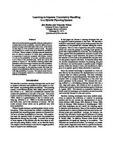
Twelve human subjects with no known neuromotor disorders consented to participate in this study. Subjects executed half-second, 20-cm reaching movements with their dominant arm in the horizontal plane while holding the handle of a two-joint, robotic manipulator (Fig. 1A). The robot was comprised of a five-bar linkage with torque motors controlled by a dedicated PC (Scheidt et al. 2000). Subjects were instructed to “reach from the beginning target to the ending target in one half second.” The computer provided qualitative feedback of movement duration after each trial (either too fast: ⬍0.45 s, too slow: ⬎0.55 s, or just right: 0.45– 0.55 s). Subjects were instructed to relax after each movement while the manipulandum moved the hand slowly back to the beginning target. This protocol was designed for allowing subjects to experience the limb’s mechanical environment along a limited set of trajectories. Reaching movements were

directed away from the subject’s body along a line (the positive y axis) passing through the center of rotation of the shoulder. The subjects’ arms were supported against gravity by a sling attached to the 8-ft ceiling. The support was adjusted so that the upper arm was abducted by 90°. The shoulders were restrained using a Velcro torso support. “Beginning” and “end” targets corresponding to a 20-cm reach in the plane of the arm were presented on a computer monitor just above the manipulandum. The position of the hand was displayed as a small cursor on the overhead monitor. Subjects could see both their arm and the cursor representing it at all times. The robotic manipulator applied perturbing force fields to the arm during each movement. A perpendicular viscous field was designed to deflect the hand perpendicularly from its intended path with a force proportional to hand velocity along its path (Fig. 1B). The forces applied to the subject’s hand during the ith movement were defined

冋 册 冋 FX FY

⫽ Bi

0 0

⫺1 0

册冋 册 x˙ y˙

(1)

where x˙ and y˙ were the two components of the hand velocity along the medial/lateral (x) and proximal/distal (y) directions, FX and FY were the two components of the force applied by the robot along the same directions. Bi was a random real number between 0 and 30 Newton second/meter (Ns/m) such that the amplitude (but not the direction) of the perturbing force field varied randomly from trial to trial. Movements were always made along the positive y direction, and perturbing forces were always directed to the left. It must be stressed that during each movement, subjects experienced variable forces that depended linearly on their instantaneous hand speed. However, the magnitude of the environmental impedance, Bi, remained constant for the duration of each individual movement and changed only between trials. Subjects could experience peak hand forces up to 30 or 40 N in this field. Subjects could perform the task easily in the time allotted; however, reaching accuracy was influenced by the perturbations. During each trial, instantaneous hand positions were recorded using rotational encoders on the robot’s motors and hand forces were recorded using a 6 degree-of-freedom load cell mounted at the handle of the robot. Two stochastic perturbation sequences were used. In experiment 1, four subjects were presented with a sequence of 200 trials in which the force-field gain, Bi (Fig. 2A), followed a Gaussian distribution (Fig. 2B). This distribution had a nonzero mean corresponding to information about the perturbation sequence that subjects might learn. The mean perturbation amplitude was 15.2 Ns/m with a variance of 24.7 Ns/m. This sequence was designed to ensure insignificant correlation between perturbation magnitudes on consecutive trials separated by more than 40 trials (Fig. 2C). The significance of each correlation term was evaluated by comparing the correlation magnitude at each

FIG. 1. A: schematic representation of the 2 degree-of-freedom robotic manipulandum used in the present experiments. B: graphical representation of the perpendicular field presented to the subjects. Perturbing forces were directed perpendicular to the direction of intended motion with amplitudes proportional to hand velocity along the intended movement direction. Force-field gains (but not direction) varied randomly from trial to trial.

J Neurophysiol • VOL

86 • AUGUST 2001 •

www.jn.org

LEARNING TO MOVE AMID UNCERTAINTY

973

FIG. 2. A: the trial-to-trial sequence of force-field gains (Bi) used in experiment 1 (4 subjects). B: unimodal Gaussian probability density function used to generate the random sequence in A. C: autocorrelation of the Gaussian sequence shown in A. The two horizontal lines correspond to the 95% confidence interval bounds (i.e., the 2␴ limits) on the correlation magnitudes. Note that no correlation term within the 1st 40 trials (except the unit autocorrelation at 0 lag) exceeded the 95% bounds to attain significance at the P ⬍ 0.05 level. D: the trial-to-trial sequence of force-field gains (Bi) used in experiment 2 (8 subjects). E: bimodal probability density function used to generate the random sequence in D. F: autocorrelation of the bimodal sequence shown in D. The two horizontal lines correspond to the 95% confidence interval bounds on the correlation magnitudes. While each unimodal subpopulation contained no significant correlations within 40 trials, the shuffling process used to combine the 2 individual populations gave rise to spurious correlations at trial lags ⬍40 trials.

integer lag value to an estimate of the 95% confidence interval bounding zero correlation (2␴ ⬵ 2/公N) (Box et al. 1994). All four subjects were exposed to the same sequence of perturbations. In experiment 2, eight subjects were presented with a sequence of 400 J Neurophysiol • VOL

trials with a bimodal probability density function (Fig. 2, D and E). This bimodal sequence was constructed by shuffling together two unimodal sequences with individual Gaussian distributions having means of 6 Ns/m (175 trials) and 25 Ns/m (225 trials), respectively.

86 • AUGUST 2001 •

www.jn.org

974

R. A. SCHEIDT, J. B. DINGWELL, AND F. A. MUSSA-IVALDI

While each individual subpopulation contained no significant correlations between perturbations separated by as many as 40 trials, the shuffling process used to construct the bimodal population gave rise to spurious correlations at trial lags ⬍40 trials (Fig. 2F). All eight subjects were exposed to the same sequence of perturbations. This bimodal stochastic perturbation sequence had greatly differing mean (15.5 Ns/m) and mode (25 Ns/m) values and was constructed to distinguish whether subjects adapt more closely to the mean or the mode of a given perturbation sequence or whether adaptation gets “trapped” in the smaller, local maximum designed into the bimodal probability distribution function.

Data analysis Simple measures of kinematic and kinetic behavior were used to assess subject motor performance on each trial during this goaldirected reaching task. “Movement error” was defined as the peak deviation of the hand from a straight-line trajectory passing between the initial and final targets (Krakauer et al. 1999). Movement error was used to quantify kinematic performance, assuming that subjects intended to make straight-line movements of their hands. This measure of motor performance has previously been found to motivate motor adaptation during reaching (Scheidt et al. 2000). The peak hand force that was generated perpendicular to the direction of movement quantified dynamic performance. An exponential function was fitted to the trial series of movement errors to characterize the rate at which subjects compensated for the random sequence of perturbation gains. This model had three free parameters: gain, A, time-constant, ␭, and offset, C E i ⫽ Ae共⫺i/␭兲 ⫹ C

(2)

where Ei was the computed movement error on trial i. The exponential captured the overall rate of change in movement error, while the constant (C) described any steady-state bias in these time series. The free parameters of this model were fit using a simplex search algorithm (Press et al. 1988). A regression analysis of movement error versus perturbation amplitude was performed to determine the field strength (i.e., perturbation gain) that subjects adapted to. The strength of correlation between these two variables and the linearity of this relationship were also evaluated. The amplitude of the field strength to which subjects adapted was estimated from the zero crossing of the resulting regression line since the perturbation gain value at which the regression line passed through zero error indicated the field strength at which subjects would exhibit error-free (straight line) trajectories. This analysis, however, provides no explanation for how subjects adapted to this particular field strength. Subjects could adapt by directly counteracting this “zero error” perturbation magnitude itself on each and every trial; i.e., by executing a control strategy that anticipated the same constant field trial after trial. If so, movement errors would vary linearly with perturbation strength. Alternatively, subjects could employ a continuously evolving strategy of using information about perturbations and movement errors from a limited number of previous trials to adjust performance on subsequent trials. Because such a strategy could also result in a linear relationship between movement error and perturbation strength, the regression analysis described in the preceding text could not distinguish these two possibilities. The preceding regression analysis was extended to evaluate the dependence of movement errors on previous perturbations and previous errors using autocorrelation and cross-correlation analyses. Specifically, the autocorrelation profile of the movement error trial sequence and the cross-correlation between the error and perturbation gain trial sequences were calculated. If subjects anticipate a constant field strength when exposed to an uncorrelated sequence of perturbations (e.g., the mean field strength), then their performance on each trial must also be uncorrelated with that of previous trials. This hypothesis was directly tested by this analysis. J Neurophysiol • VOL

These correlation analysis results were then used to guide construction of a model of motor adaptation during reaching. Specifically, movement error on each trial was modeled as a linear combination of previous movement errors as well as present and previous perturbation amplitudes. The result was a parametric model of motor adaptation that was linear in its inputs

冘 i⫺L

⑀i ⫽

冘

i⫺M

aj ⑀i⫺j ⫹

j⫽1

bk Bi⫺k

(3)

k⫽0

where aj and bk were coefficients weighting the relative importance of previous errors (⑀i-j) and previous perturbation magnitudes (Bi-k) on subsequent errors, j and k were indices of summation while L and M were limits on the number of significant terms in the model. Values for L and M were obtained directly from the correlation analysis. This model represents an autoregressive process with external input (i.e., an ARX model) (Ljung 1999). Terms with nonzero aj coefficients are autoregressive terms because they define the dependence of the current movement error on previous movement errors. Terms with nonzero bk coefficients are moving average terms of the external input because they define the dependence of the current movement error on a sliding window average of current and previous perturbation amplitudes. Because Eq. 3 defines a discrete-time difference equation, the stability and steady-state behavior of this model of motor adaptation was analyzed using z transform techniques (Oppenheim and Schafer 1989). The capacity of this model to predict subjects’ adaptation to the random sequence of perturbations was evaluated. These predictions were compared with the predictions of two alternate, but viable, learning algorithms. The first alternative model accumulated an explicit representation of the mean perturbation strength by “memorizing” the perturbation sequence trial by trial. This explicit representation of the running-average mean perturbation was used to compensate for the perturbation on the next trial. The second alternative model was an incremental learning algorithm that utilized local weighting of the most recent movement errors to predict and compensate for the magnitude of the next perturbation. This model included the possibility of nonuniform and nonlinear attention models whereby learning could either attend closely to or ignore trials where the perturbation amplitude was “surprising” or “irrelevant” (Atkeson et al. 1997). Each model was first fit from the subjects’ data from the initial 100 movements in the experiments. The performance of each model was then evaluated according to its ability to predict subject movement errors on the last 100 movements. Model performance was quantified using the variance accounted for (VAF) as a measure of goodness-of-fit VAF ⫽ 1 ⫺

var 共residuals兲 var 共data兲

(4)

RESULTS

Subjects compensate for the approximate mean of the random trial sequence of perturbations An overhead view of averaged hand paths made during experiment 1 (Fig. 3A; unimodal perturbation sequence) shows that subjects exhibited substantial kinematic deviations to both the left and right even though they experienced forces that pushed only to the left. To compare across trials, hand-path data were aligned with respect to the onset of movement (the point in time when hand speed first exceeded 0.1 m/s; Fig. 3B) and averaged into six “bins” of 5 Ns/m width each (0 –5, 5–10, 10 –15, etc.). Movements from trials with field strengths ⬎20 Ns/m resulted in trajectories that deviated markedly to the left (i.e., in the direction of the applied force). However, hand-path deviations were con-

86 • AUGUST 2001 •

www.jn.org

LEARNING TO MOVE AMID UNCERTAINTY

975

FIG. 3. Results from experiment 1 (unimodal perturbation sequence). A: overhead view of averaged hand paths from 1 subject across the entire experiment. Trials were averaged into 6 “bins” of 5 Ns/m width (0 –5, 5–10, 10 –15, etc.). Trials with field strengths ⱖ25 Ns/m were undercompensated (left-most profile), while trials with field strengths ⱕ5 Ns/m were overcompensated (right-most profile). Movements were truncated at the point of time near the end of movement where the hand speed profile reached a transient minimum. Average trajectories after the time of truncation are shown with triangular symbols. B: average hand speed profiles for the same subject. The vertical dashed line indicates the approximate time at which hand speed reached a transient minimum, separating the hand speed profile into 2 peaks. C: movement errors for this subject plotted against trial number. The dark, solid line represents the exponential best-fit estimate of movement error (Eq. 2). D: perpendicular hand force profiles obtained by averaging the data in the same manner as in A and B. E: scatter plot of movement error vs. perturbation strength, exhibiting a nearly linear relationship (r ⫽ 0.82). F: best-fit linear regressions from the scatter plots of all subjects from experiment 1 (0.73 ⬍ r ⬍ 0.84).

sistently toward the right (i.e., opposite to the direction of the applied force) for fields with gains ⬍10 Ns/m. Movements made in weaker fields had hand-path errors that were approximately mirror symmetric to those made in stronger fields. Kinematic errors made in the weakest fields were nearly identical to responses observed when perturbing force fields were unexpectedly removed after adaptation (Scheidt et al. 2000). This finding is consistent with traditional measures of aftereffects of adaptation J Neurophysiol • VOL

(Shadmehr and Mussa-Ivaldi 1994). These aftereffects are a clear indication that subjects compensated for the perturbations by adopting some automatic and predictive mechanism. Force fields roughly corresponding to both the mean (average) and mode (most likely) disturbance (10 –15 Ns/m) resulted in movements with the least curvature. Note that these movements were only approximately straight, corresponding to the steady-state bias in movement error (constant C in Eq. 2).

86 • AUGUST 2001 •

www.jn.org

976

R. A. SCHEIDT, J. B. DINGWELL, AND F. A. MUSSA-IVALDI

Average hand speed profiles (Fig. 3B) typically demonstrated two distinct peaks. The secondary peak in the hand speed profile could be the result of several mechanisms including, but not limited to, active correction under visual feedback, reflex-mediated adjustments due to the mismatch between the intended and actual final joint posture (the mismatch being due to the perturbation) or the interaction of limb and manipulandum dynamics (Shadmehr and Mussa-Ivaldi 1994). The present experiment was not designed to distinguish between these alternatives. Therefore movements were truncated at the point of time near the end of movement where the hand speed profile reached a transient minimum (vertical line in Fig. 3B, solid lines in Fig. 3A returning to final target location). This limited subsequent analysis to the portion of movement that was predominantly feedforward. An exponential function (Eq. 2) was fit to the movement error trial series (dark solid line in Fig. 3C), confirming the presence of a steady-state bias in movement error. Figure 3C shows a rapid decrease in movement error within the first 10 –20 trials (time constant ⫽ 2.4 trials). Time constants (␭ in Eq. 2) for all four subjects averaged 3.2 ⫾ 0.74 trials (mean ⫾ SE mean). The residual steady-state movement error (constant C in Eq. 2) was observed in all four subjects (average 12.3 ⫾ 2.7 mm), indicating that subjects compensated only approximately for the mean of the random trial sequence. These observations were consistent across all four subjects exposed to the unimodal perturbation sequence. Subjects did indeed adapt in response to the random sequence of perturbations. Profiles of the hand forces generated perpendicular to the direction of movement (Fig. 3D) provide further evidence of adaptation to the stochastic sequence of perturbations. Subjectgenerated forces dominated movements made in the weakest fields (the smallest force profile with biphasic shape), whereas robot-generated forces dominated movements made in the strongest fields (the largest profile with monophasic shape). The initial peak in perpendicular force generated by the subject in the weakest field (⬃12 N) was directed opposite to the forces imposed by the robot and was not necessary to move the hand toward the target. This excessive force caused the limb to deviate substantially from the target, producing a kinetic aftereffect of adaptation. Consequently, restoring forces (the negatively directed peak in Fig. 3E) were required to move the limb to the final target. An analysis of movement error versus perturbation amplitude (Fig. 3, E and F) indicated that these two variables were well fit by a linear relationship within the range of our experiment (r ⫽ 0.82 in Fig. 3E; 0.73 ⬍ r ⬍ 0.84 for all 4 subjects). The point of zero error on these regression lines indicates the field strength that was best compensated for through the adaptive process (13.5 Nm/s in Fig. 3E; 12.9 ⫾ 1.2 Ns/m for all 4 subjects in Fig. 3F). This adapted field strength approximated, but did not quite attain, the mean value of the distribution (P ⬍ 0.01; Student’s t-test rejecting the null hypothesis H0: Badapt ⫽ B៮ ⫽ 15.2 Ns/m). Thus subjects compensated for force fields somewhat less than (but coarsely approximating) the mean gain (i.e., Bi ⬇ B៮ ), greatly undercompensated large force-field gains (i.e., Bi ⬎⬎ B៮ ), and greatly overcompensated small forcefield gains (i.e., Bi ⬍⬍ B៮ ). J Neurophysiol • VOL

Adaptation to the approximate mean, not to the mode An overhead view of averaged hand paths made by one subject from experiment 2 (Fig. 4A; bimodal perturbation sequence) shows that again, movements were either deflected to the left or to the right. Average hand speed profiles (Fig. 4B) exhibited the same biphasic pattern found in experiment 1. Consequently, the data from experiment 2 were truncated in same way as in experiment 1. The truncated and averaged hand movements (Fig. 4A) exhibited consistent deviations toward the right when movements were made in fields with strengths of ⱕ10 Ns/m and toward the left when movements were made in fields with strengths of ⱖ20 Ns/m. Force fields roughly corresponding to the mean disturbance (10 –15 Ns/m) resulted in trajectories with the least curvature although they were not ideally straight. These results demonstrate that adaptation to a sequence of perturbations with randomly varying magnitudes converges to the approximate mean perturbation magnitude rather than the most likely magnitude. Fitting an exponential function (Eq. 2) to the movement error trial series (dark solid line in Fig. 4C) produced results that varied widely across subjects [time constant ␭ ⫽ 54.8 ⫾ 18.2 (SE) trials; range ⫽ [11.2, 167] trials; n ⫽ 8]. Consequently, this traditional measure of learning suggests that the bimodal perturbation sequence abolished (or at least slowed) the initial rapid learning observed in experiment 1. However, as shown in the following text, subject performance in both experiments can be described using a single, parsimonious description of motor adaptation. Figure 4D displays average perpendicular hand force profiles measured at the handle in the bimodal experiment. The overall shape of the profiles was similar to those observed in the unimodal experiment with the initial peak in perpendicular force generated in the weakest fields giving rise to the undesirable deviation from the target indicative of aftereffects of adaptation. Again this is a kinetic aftereffect of adaptation similar to that observed in the first experiment. As in the unimodal experiment, the hand force profiles were smooth and the restoring forces generated at the end of the movement did not appear to be distinct pulses. As in the unimodal experiment, subjects exposed to the bimodal perturbation sequence exhibited a linear relationship between movement error and perturbation strength (r ⫽ 0.85 in Fig. 4E; 0.83 ⬍ r ⬍ 0.94 for all 8 subjects). Again, the point of zero error on these regression lines was taken as the field strength that was best compensated for through the adaptive process. These eight subjects adapted to an average field strength of 11.33 Ns/m with a 95% confidence interval of [8.61, 14.04] Ns/m (Fig. 4F). For all eight subjects, the major and minor peaks of the bimodal probability density function (6 and 25 Ns/m, respectively) both fell outside this 95% confidence interval. However, although the adapted field strength in the bimodal sequence was substantial, subjects did not quite compensate for the mean perturbing field (B៮ ⫽ 15.5 Ns/m), even after 300 – 400 movements. Somewhat paradoxically, subjects actually adapted to a perturbing field strength that was experienced rarely. Only recent memories contribute to adaptation The Gaussian-distributed random trial sequence (Fig. 2, A and B) was used to perturb subjects while adapting because this

86 • AUGUST 2001 •

www.jn.org

LEARNING TO MOVE AMID UNCERTAINTY

977

FIG. 4. Results from experiment 2 (bimodal perturbation sequence). A: overhead view of averaged hand paths from 1 subject. Trials were averaged into 6 bins of 5 Ns/m width (0 –5, 5–10, 10 –15, etc.). As in experiment 1, trials with field strengths ⱖ25 Ns/m were undercompensated (left-most profile), whereas trials with field strengths ⱕ5 Ns/m were overcompensated (right-most profile). Movements were truncated at the point of time near the end of movement where the hand speed profile reached a transient minimum. Average trajectories after the time of truncation are shown with triangular symbols. B: average hand speed profiles for the same subject. The vertical dashed line indicates the approximate time at which hand speed reached a transient minimum, separating the hand speed profile into 2 peaks. C: movement errors for this subject plotted against trial number. The dark, solid line represents the exponential best-fit estimate of movement error (Eq. 2). Note that movement error was not well fit by a falling exponential function in the bimodal experiment. D: perpendicular hand force profiles obtained by averaging the data in the same manner as in A and B. E: scatter plot of movement error vs. perturbation strength, exhibiting a nearly linear relationship (r ⫽ 0.85). F: best-fit linear regressions from the scatter plots of all subjects from experiment 2 (0.83 ⬍ r ⬍ 0.94).

input to the motor adaptation process was both uncorrelated from trial to trial (up to a lag of 40 trials; Fig. 2C) and “rich” spectrally (Marmarelis and Marmarelis 1978). Driving each subject’s motor system with an uncorrelated trial sequence ensured that any trial-to-trial correlations observed in that subject’s motor output did not originate from the perturbation sequence but rather from information processing within the J Neurophysiol • VOL

neuromotor controller. Despite this lack of correlation in the sequence of perturbing fields, significant trial-to-trial correlations were observed in subjects’ motor output (Fig. 5). Correlations between movement error and perturbation gain (Fig. 5A) exceeded statistical significance (⬎95% CI) not only on concurrent trials (i.e., lag ⫽ 0) but also on the preceding trial (lag ⫽ ⫹1). The sign of the correlation at lag 1 was opposite

86 • AUGUST 2001 •

www.jn.org

978

R. A. SCHEIDT, J. B. DINGWELL, AND F. A. MUSSA-IVALDI

FIG. 5. Correlation analysis of motor performance during adaptation for a typical subject from experiment 1. A: cross-correlation magnitude between movement error and perturbation gain. Horizontal lines correspond to 95% confidence interval bounds (i.e., the 2␴ limits) on the correlation magnitudes. Movement error on a given trial correlated with perturbation gain on that same trial and with perturbation gain on the previous trial as subjects compensated for the most recently experienced perturbation. B: autocorrelogram of movement error. Movement error on a given trial correlated with movement error on the previous trial. C: cross-correlation magnitude between peak perpendicular hand force and the perturbation gain, exhibiting a lag-1 correlation with perturbation amplitude. D: cross-correlation magnitude between peak perpendicular hand force and movement error, which also exhibited a significant correlation with previous movement error (lag ⫽ ⫹1), consistent with A.

that at lag 0, indicating that subjects attempted to reduce movement error on each trial by countering the previous perturbation. Significant correlations between movement error and perturbation gain extended back no more than two trials for all of the four subjects exposed to the perturbation sequence with the unimodal distribution. Movement errors on a given trial also exhibited substantial correlations with errors generated in the preceding trial (Fig. 5B). By definition, the autocorrelation function is symmetric about 0 lag. Thus correlations at any given lag are reflected at the corresponding lead with no violation of causality. Significant autocorrelation terms were found at a lag of one trial for three of the four subjects (the remaining subject showed no significant correlations beyond lag 0). Again, the sign of this correlation was negative indicating that subjects attempted to reduce movement errors on each trial by countering movement errors generated on the previous trial. Similar correlation analyses were performed on the peak hand forces generated perpendicular to the intended direction of movement (Fig. 5, C and D). Correlations between peak hand force and perturbation gain (Fig. 5C) exceeded statistical J Neurophysiol • VOL

significance (⬎95% CI) only on concurrent trials (i.e., at 0 lag) and at a lag of one trial. Significant correlations between peak hand force and perturbation gain extended back no more than two trials for all four subjects in experiment 1. Correlations between movement error and peak hand force (Fig. 5D) exceeded statistical significance only on concurrent trials and, at a lag of one trial, a result entirely consistent with the findings of Fig. 5A. The significant correlations at zero lag (Fig. 5, A, C, and D) were due in part to mechanical interaction between the robot and the finite impedance of the subject’s arm. Larger forces imposed by the robot on the hand resulted in both larger deviations of the hand from its intended path and in greater forces being recorded at the handle. However, significant correlations at nonzero lags cannot be explained by mechanical interactions. These lag 1 correlations indicate that subjects used explicit information regarding the strength of the perturbation from the previous trial to preprogram the motor response on each subsequent trial. Subjects also utilized information about previous performance to update motor behavior on subsequent trials. The lack of significant correlations be-

86 • AUGUST 2001 •

www.jn.org

LEARNING TO MOVE AMID UNCERTAINTY

yond two previous trials indicates that explicit memory representation of more remote trials was not used during motor adaptation. Had subjects adapted to the stochastic sequence of perturbations by directly counteracting some constant field strength on each trial (e.g., the mean), their motor output would likewise be uncorrelated with the input. This hypothesis is clearly refuted by the present findings. These findings support the hypothesis that explicit information of only one or two previous trials is sufficient to allow subjects to compensate for the approximate mean field strength in a random sequence of perturbations. Predicting motor performance The preceding analyses suggest that subject performance (quantified by movement error) exhibited on any given trial, i can be predicted solely from the field strength on that trial (Bi) and from the field strength and error exhibited on the previous trial (Bi-1 and ⑀i-1, respectively) ⑀ i ⫽ a1⑀i⫺1 ⫹ b0Bi ⫹ b1 Bi⫺1

(5)

Regression coefficients (a1, b0, b1) were estimated over the initial 100 trials for each subject in experiments 1 and 2 by performing a multi-linear regression of movement error on previous movement errors, previous perturbations and concurrent perturbations (Table 1). The ability of this model to predict movement error in the last 100 movements in each experimental session was evaluated to determine how well the model would generalize beyond the data set used to determine model coefficients. The ability of this model to predict performance for greatly differing perturbations sequences (i.e., unimodal vs. bimodal distribution) was also evaluated. Model performance was quantified using the variance accounted for (VAF; Eq. 4). The percentage of VAF by this model from the unimodal experiment was 79% for the subject shown in Fig. 6A and 71 ⫾ 3% (mean ⫾ 1 SE) for all four subjects. The percentage of VAF by this model from the bimodal experiment was 86% for the subject shown in Fig. 6B and 84 ⫾ 2% for all eight subjects. Thus a model incorporating limited explicit memory of subject performance and perturbation magnitudes can predict movement errors with a high degree of fidelity. This strongly suggests that motor adaptation is a continuously evolving process whereby the average field in a sequence of TABLE

Subject U1 U2 U3 U4 B1 B2 B3 B4 B5 B6 B7 B8 U B

979

perturbations is compensated using properly weighted cancellation of both previous perturbation amplitudes and previous movement errors. Step response analysis Although the model performed quite well in response to the stochastic input sequences from which it was originally derived, it was also important to determine how well this model could predict behavior exhibited in response to nonstochastic sequences of input perturbations. Equation 5 was used to simulate movement errors in response to a step increase in perturbation strength that included a simulated “catch trial” near the end of the input sequence (Fig. 7A, top). This input sequence was specifically designed to mimic the constant force field gains and catch trials used in previous motor adaptation experiments (e.g., Shadmehr and Mussa-Ivaldi 1994). Average coefficient values from the unimodal experiment (Table 1) were used to define the model parameters. When presented with a step increase in perturbation strength, the simulated movement errors rapidly approached their asymptotic value (within 3– 4 trials) and exhibited a small steady-state error at large trial numbers as did subjects in both experiments. The model output also exhibited the classic behavior of an “aftereffect” (Shadmehr and Mussa-Ivaldi 1994) when the catch trial was introduced at trial number 75. Furthermore, this model was also able to account for the observations of Thoroughman and Shadmehr (2000) that a single catch trial can transiently degrade the adapted state generated in response to a consistent perturbing field. Consequently, this very simple model of motor adaptation succinctly captures the fundamental behavioral characteristics exhibited in both the present experiment and in more traditional experiments of motor adaptation. Interpretation of model coefficients To investigate how each term of the model related to observed behaviors, the output of the model in response to the same step input (Fig. 7A) was analyzed for various combinations of model parameters (Fig. 7B). A model that does not rely on prior experience, and thus has no memory (i.e., a1 ⫽ b1 ⫽ 0; trace 1), can only respond to the current perturbation and fails to adapt. This is the response one would expect if subjects were only co-contracting their limb in response to the pertur-

1. Equation 5 regression coefficients and goodness-of-fit measures for both the unimodal and bimodal experiments n

a1

b0

b1

VAF

r

4 8

0.29 0.43 0.45 0.09 0.53 0.52 0.39 0.49 0.29 0.52 0.53 0.62 0.31 ⫾ 0.11 0.49 ⫾ 0.04

⫺2.43 ⫺3.99 ⫺5.37 ⫺3.84 ⫺4.29 ⫺2.55 ⫺4.32 ⫺4.40 ⫺3.27 ⫺3.25 ⫺3.92 ⫺5.59 ⫺3.91 ⫾ 0.60 ⫺3.95 ⫾ 0.33

1.94 3.73 4.66 2.85 2.23 2.62 3.47 3.35 1.94 2.68 3.27 4.57 3.29 ⫾ 0.58 3.02 ⫾ 0.29

0.62 0.73 0.77 0.70 0.87 0.80 0.86 0.86 0.81 0.77 0.86 0.92 0.71 ⫾ 0.03 0.84 ⫾ 0.02

0.79 0.85 0.88 0.84 0.93 0.89 0.93 0.93 0.90 0.88 0.93 0.96 0.84 ⫾ 0.02 0.92 ⫾ 0.01

U and B values are means ⫾ SE. J Neurophysiol • VOL

86 • AUGUST 2001 •

www.jn.org

980

R. A. SCHEIDT, J. B. DINGWELL, AND F. A. MUSSA-IVALDI DISCUSSION

The present experiments investigated the ability of unimpaired humans to adapt to a viscous, perpendicular, force-field environment having force-field gains that were unpredictable (and uncorrelated) from trial to trial. Experiments were designed to determine if subjects adapted to the mean force field gain, the most likely field, or whether adaptation would depend on other features of the perturbation sequence’s probability density function. Correlation analyses were performed to determine how much motor performance on any given trial was correlated with performance on previous trials. It was found that 1) subjects adapted their motor behavior in response to the random sequence of force field gains, 2) subjects compensated

FIG. 6. Within-subject comparison of predicted (ARX model; Eq. 5) movement errors with actual movement errors during the final 100 movements of the experiment. Model parameters were evaluated from the 1st block of 100 trials. A: prediction of performance for a typical subject in the unimodal perturbation sequence. The dark line represents actual subject performance, while the thin line represents the model prediction. The model accounted for 79% of the data variance. B: prediction of subject performance in the bimodal perturbation sequence (same line types as in A). The model accounted for 89% of the data variance.

bations. Increased co-contraction might decrease the magnitude of the b0 term, but unless the limb stiffness became exceedingly large, a substantial residual offset would remain. The amount of residual steady-state error in the adaptive response is determined by the relative magnitudes of b0 and b1. When b0 ⫽ ⫺b1 (trace 2), then the residual steady-state error is eliminated. On the other hand, when the autoregressive term in the model is removed (a1 ⫽ 0; trace 3), the dynamics associated with initial exposure to the perturbation are eliminated while the steady-state error is reduced relative to the full model (Fig. 7A). If this autoregressive term is instead doubled (trace 4), the initial transients are extended and the steady-state error is increased. Changing the sign of a1 (traces 5 and 6) does not alter the time course of adaptation but causes the model’s response to oscillate within the envelope defined in Fig. 7, A (bottom) and B (trace 4), respectively. Note, however, that changing the sign of a1 does in fact reduce (but not eliminate) the steady-state error. Finally, not all choices of parameters yield stable learning. Setting a1 ⬎ 1.0 yields an unstable algorithm that never adapts (trace 7). J Neurophysiol • VOL

FIG. 7. Step response analysis of a family of autoregressive models based on Eq. 5. The coefficients for each model are described above the corresponding response curves. A, top: input sequence corresponding to a step increase in the strength of force-field perturbation, similar to the perturbations traditionally used to study motor adaptation. Note that a “catch trial” (impulse) was included near the end of the sequence to allow a direct comparison of the model’s response to catch trial behavior described in the text. A, bottom: response of a model derived from the average coefficients of the 4 subjects participating in the unimodal experiment. Note that the model exhibits a steady-state error as trial numbers become large as did subjects in both experiments. B: 1: step response of a model with no memory; the response on any given trial is only dependent on the current perturbation magnitude; 2: response of a model that precisely compensates for the most recent perturbation without either attenuation or amplification; b1 ⫽ b0. 3: response of a model with no autoregressive term; a1 ⫽ 0. 4: response of a model with its autoregressive term doubled; 5: model response when the sign of the autoregressive term has been inverted; 6: model response when the autoregressive term has been both inverted and doubled. 7: response of an unstable model a1 ⬎ 1.0.

86 • AUGUST 2001 •

www.jn.org

LEARNING TO MOVE AMID UNCERTAINTY

for the approximate mean field of the stochastic sequence, not the most likely field, and 3) subjects compensated using memories of only the most recent perturbations and the most recent performances. What did subjects adapt to? Subjects experienced perturbing forces that were always directed toward their left. If no adaptation had occurred, then all movement errors would likewise have been directed toward the left. However, for field strengths of ⬍10 Ns/m, hand-path deviations were made consistently toward the right in both experiments (Figs. 3A and 4A). The presence of these oppositely directed errors (i.e., to the right) indicates that subjects were directly opposing forces they anticipated encountering and precludes the possibility that they were merely stiffening the arm around some reference trajectory (Conditt et al. 1997a; Flash 1987; Shadmehr and Mussa-Ivaldi 1994). Furthermore movements made in stronger-than-average force fields were undercompensated, whereas movements made in weaker-thanaverage force fields were overcompensated, suggesting that subjects were compensating approximately for the mean perturbing force field in both experiments. This finding was confirmed by linear regression analysis (Figs. 3E and 4E). Learning rates in the present study (Figs. 3C and 4C) were slower than rates reported for compensation of inertial loads (within 1 trial) (Bock 1993) but were substantially faster than learning rates reported for consistent (but geometrically complex) viscous environments when subjects were required to reach in several different directions (more than 100 trials) (Bhushan and Shadmehr 1999). Remarkably, the learning rates observed in experiment 1 were almost identical to the rates at which subjects regained adaptation to a predictable perturbing environment after a single “catch trial” in which the perturbing environment was unexpectedly removed (⬃3 trials) (Thoroughman and Shadmehr 2000). Clearly, subjects adapted to these stochastic environments. Adaptation modeled as an autoregressive process with external input (ARX process) Although the linear regression results demonstrated that subjects compensated for the approximate mean perturbation strength in both force-field environments, they did not suggest how the central nervous system accomplished this adaptation. Mathematically, the mean perturbation magnitude is defined as the sum of the individual magnitudes divided by the number of perturbations. Since subjects had no way of knowing all of the perturbation magnitudes until the experiment was completed, it was not possible for them to directly compute the mean field strength. Subjects could have evaluated a “running average” of all trials they experienced so far. However, this strategy would require subjects to retain either explicit working memory of all previously encountered perturbations or explicit memory of the average of all previous perturbations along with a running total of the number of previous perturbations. In either case, the relative importance of the most recent perturbation would decrease linearly as a function of the number of perturbations. A less demanding alternative would be for subjects to rely only on explicit information regarding only recent experiences. Motor performance (and consequently motor adaptation) may J Neurophysiol • VOL

981

rely on information about past movement performance and/or past perturbations derived from a variety of sensory sources (e.g., muscle spindles, Golgi tendon organs, slowly adapting hand mechanoreceptors, vision, etc.). A general form of this model, one that depends only on information regarding movement errors and perturbation amplitudes (Eq. 3) was examined in the present experiment. One important aspect of this model is that information about experiences in the distant past is retained implicitly in the autoregressive terms (i.e., if Eq. 3 contains at least one nonzero aj term). The correlation analyses (Fig. 5) demonstrated that movement error on a given trial i was well predicted from the field strength on that trial (Bi) and from the field strength (Bi-1) and movement error (⑀i-1) exhibited on the previous trial (Eq. 5). Why do subjects compensate for previous movement errors when the step response analysis suggests that learning would be more rapid and effective if those errors were disregarded altogether (i.e., set a1 ⫽ 0 in Eq. 5) and the most recent perturbation was canceled exactly (i.e., set b1 ⫽ ⫺b0 in Eq. 5; Fig. 7B, trace 2)? Are there unavoidable history dependencies in the proprioceptive and/or visual sensory pathways that constrain the motor learning mechanisms in their “choice” of compensatory strategies? It has been suggested that cancellation of prior movement errors is important to motor adaptation (e.g., Flanagan and Rao 1995; Scheidt et al. 2000; Wolpert et al. 1995). Equation 5 suggests that compensating for the most recent movement error exactly (i.e., a1 ⫽ ⫺1 in Eq. 5) would be a counter-productive strategy since Eq. 5 becomes unstable when 兩a1兩 ⱖ 1. This can be seen by examining the stability of Eq. 5 in the complex z-domain (Oppenheim and Schafer 1989). The z transform of Eq. 5 is E共z兲 ⫽ a1z⫺1E共z兲 ⫹ b0B共z兲 ⫹ b1z⫺1B共z兲

(6)

Consequently, the model’s transfer function H(z) is H共z兲 ⫽

E共z兲 共b0 ⫹ b1z⫺1兲 ⫽ B共z兲 共1 ⫺ a1z⫺1兲

(7)

H(z) has a zero at z ⫽ ⫺b1/b0 (see Fig. 7B, trace 2) and a single, real pole situated at z ⫽ a1. The location of the zero in the unimodal and bimodal experiments was not significantly different at the P ⬍ 0.05 level (P ⫽ 0.39; 2-sample t-test), and the location of the system pole in the two experiments was also not significantly different (P ⫽ 0.13). Therefore to the extent that this linear model captures the mechanisms of adaptation, we conclude that the process of adaptation is not sensitive to the details of the distribution of the perturbing forces (e.g., mode, skewness, etc.), but only to its mean. The location of the zero at z ⫽ ⫺b1/b0 is significant because in the steady state (i.e., when z ⫽ 1) the transfer function is minimized when b1 ⫽ ⫺b0. Furthermore, for any linear system to be stable, all the poles of its transfer function must lie within the unit circle defined in the complex z plane (i.e., 兩z兩 ⬍ 1) (Oppenheim and Schafer 1989). Therefore 兩a1兩 ⬍ 1 must be satisfied for Eq. 5 to be stable. Perfect cancellation of the most recent movement error (i.e., a1 ⫽ 1) would cause the motor adaptation process to become unstable (e.g., Fig. 7B, trace 7). Explicit representation of the internal model Since the relationship between movement error and perturbation gain was reasonably well fit by a straight line (Figs. 3E

86 • AUGUST 2001 •

www.jn.org

982

R. A. SCHEIDT, J. B. DINGWELL, AND F. A. MUSSA-IVALDI

and 4E), the ARX model of subject performance (Eq. 5) was rearranged to yield an expression for the internal model of the perturbing environment. Specifically, movement error generated on trial i was regarded as a function of the mismatch between the actual perturbation experienced on that trial and the expected (or adapted) perturbation magnitude: ⑀i ⫽ f(Bi ⫺ Badapted). Figures 3E and 4E demonstrate that this relationship was reasonably described by a linear function ⑀ i ⫽ k共Bi ⫺ Badapted兲

(8)

Re-arranging Eq. 5 into the form of Eq. 8 yields

冉

⑀ i ⫽ b0 Bi ⫹

冊

a1 b1 ⑀i⫺j ⫹ Bi⫺k b0 b0

⫽ b 0共Bi ⫺ Badaptedi兲

(9A) (9B)

where B adaptedi ⫽ ⫺共a1/b0兲⑀i⫺1 ⫺ 共b1/b0兲Bi⫺1.

(10)

Equation 10 provides a very simple representation of the subject’s prediction of the perturbation magnitude on trial i based solely on explicit information about the error and perturbation magnitude on the most recent trial. However, even this simple representation faithfully reproduced subjects’ behavior in the present experiment (Fig. 6). It is worth noting that parameters estimated from the first 100 trials adequately accounted for the time series of errors up to 300 trials following parameter estimation. Thus the adaptive behaviors observed in both the unimodal and bimodal experiments (Figs. 3 and 4) were a consequence of the dynamics of a quasi-stationary process with very limited memory. Motor performance would be optimized by tuning the coefficients a1, b0, and b1. Both the rate of adaptation and the steady-state error can be altered by appropriate modification of these coefficients (Fig. 7).

ing the most recent perturbation strength would be to do so indirectly and recursively, using only the most recent movement error to update the previous estimation of the perturbing field. In this case, Eq. 10 can be reformulated B adaptedi ⫽ ⫺共a1/b0兲⑀i⫺1 ⫺ 共b1/b0兲Badaptedi⫺1

Here, movement errors drive the formation of the internal model of the perturbations. Substituting the z transform of Eq. 11 into the z transform of Eq. 9B for Badapted (z) yields a transfer function that is identical in structure to Eq. 7 except that the algorithm’s single pole location is shifted to z ⫽ a1 ⫺ (b1/b0). The coefficient values that ensure stability of the system are therefore: 兩a1 ⫺ (b1/b0)兩 ⬍ 1. Using Eq. 11 and the modified Eq. 9B to fit subject U2’s movement error data yields the coefficients: a1 ⫽ ⫺0.34, b0 ⫽ ⫺4.2, b1 ⫽ 4.0. The effective pole location for this system was z ⫽ 0.62 (compare to Fig. 7B, trace 4). Since recursive estimation of Bi-1 via Eq. 11 does not alter the transfer function structure of Eq. 7, the correlation analyses of Fig. 5 cannot distinguish between recursive estimation of Badapted (Eq. 11) and estimation of Badapted via proprioception of Bi-1 (Eq. 10). Consequently, while force feedback gain from Golgi tendon organs is likely to be quite low (cf. Houk and Rymer 1981), such information is not necessary to construct an internal model of the perturbing force field environments. Comparison of the simple autoregressive model with alternative learning strategies If movement error is linearly related to the perturbing field amplitude, ⑀i ⫽ k(Bi ⫺ Badapted), then the optimal internal model in terms of least square error (i.e., the Badapted that minimizes the sum of ⑀2i ) is given by the mean field B optimali ⫽

How do the motor adaptation mechanisms estimate the most recent movement error and perturbation strength? Constructing the internal representation of the perturbing field strength via Eq. 5 requires accurate estimation of ⑀i-1 and Bi-1. Movement error is likely to be sensed both visually (e.g., Wolpert et al. 1995) and proprioceptively (Dizio and Lackner 2000; Shadmehr and Mussa-Ivaldi 1994). The current experiments were not designed to evaluate the relative contributions of different feedback modalities to motor adaptation but rather to explore how the neural mechanisms involved in motor adaptation use information from previous movements (however that information is sensed) to modify motor commands on subsequent movements. Both visual and proprioceptive feedback appear to be important (Conditt et al. 1997b), although it is not yet clear how this feedback information is combined in driving motor adaptation. There are at least two ways the CNS could estimate the most recent perturbation strength in keeping with the spirit of Eq. 10. The first strategy would be to estimate the field strength directly using sensory organs sensitive to the kinetic demands of the task (e.g., Golgi tendon organs, hand mechanoreceptors, and indirectly, muscle spindle receptors since they are coupled to the perturbation through limb tissues with finite impedance). In this case, Bi-1 would be “measured” directly and Eq. 10 would be implemented as written. The second way of estimatJ Neurophysiol • VOL

(11)

1 i⫺1

冘 i⫺1

Bj

(12)

j⫽1

In the present study, movement errors were linearly related to perturbation amplitude (Figs. 3E and 4E). This finding supports the empirical claim that subjects adapted their reaching movements so as to minimize deviations from a rectilinear path (Shadmehr and Mussa-Ivaldi 1994). One plausible alternative to the learning strategy described by Eq. 5 would be for subjects to “explicitly” learn the mean. In this case, Eq. 12 is substituted into Eq. 5 for Bi-1 while the dependence on previous movement errors (the ⑀i-1 term) is dropped ⑀ i ⫽ b0 Bi ⫹ b1 Boptimal

(13)

Equation 13 was fit to subject U2’s initial perturbation and movement error data set (1st 100 movements). The model’s performance was then evaluated in the final 100 movements of the experiment (Fig. 8A). This algorithm performed respectably when perfect memory of all perturbations encountered was available (VAF ⫽ 70%). This algorithm also quickly converged to the (ideally) linear relationship between perturbation gain and movement error (Fig. 8B). However, this model failed to exhibit the significant lag 1 correlations between movement error and perturbation amplitude observed experimentally (compare Fig. 8C to Fig. 5A). The absence of these lag 1 correlations arises from the fact that when all previous movements are considered explicitly, the contribution

86 • AUGUST 2001 •

www.jn.org

LEARNING TO MOVE AMID UNCERTAINTY

of any one individual perturbation to the internal model of the mean field becomes vanishingly small after only a few trials. Therefore the simple adaptive mechanism of Eq. 10 permits subjects to achieve near optimal performance (i.e., approximately minimizing squared errors) while maintaining computational efficiency since the autoregressive Eq. 10 approximates the ideal average of Eq. 12 with a very limited number of memory elements. (The autoregressive term in Eq. 10 retains indirect and exponentially weighted memory of all past perturbations due to the nested dependence of ⑀i-1 on previous errors.) Note also that Eq. 12 defines optimal performance only

983

when the underlying distribution of Bi is stationary. In the nonstationary case (such as the step input of Fig. 7A), the model of Eq. 12 would respond very slowly since the incremental contribution from each subsequent trial decreases progressively as the number of trials increases. Consequently, adaptation in the sense of Eq. 5 strikes a desirable compromise between decreasing movement errors in a stationary but potentially unpredictable environment while allowing the motor system to respond rapidly and appropriately to long-term changes in the perturbing environment (Fig. 7A). A second alternative learning strategy describes what could be called “careless learning” and was motivated in part by the observation that subjects never made ideally straight movements and almost always had peak hand deviations exceeding ⬃1 cm (Figs. 3E and 4E). Perhaps subjects considered movements with such small errors “good enough” for the specified task? This form of learning is careless in the sense that the learner does not attend to small movement errors. The internal representation of the perturbation in a careless learning model would be updated only when the learner is “surprised” (i.e., when the movement errors experienced on a given trial exceed a minimum threshold value, ⑀threshold). An attention model that describes how well movement errors are attended to is U共⑀i兲 ⫽ u共⑀i ⫺ ⑀threshold兲

(14)

where u(䡠) is the unit step function. The update rule for the internal model then becomes

冋冉

Bˆ adaptedi ⫽ Bˆadaptedi⫺1 ⫹ U共⑀i兲

冊

册

a1 ⫺b1 ⫺ 1 Badaptedi⫺1 ⫺ ⑀i⫺1 b0 b0

(15)

Note that if ⑀threshold ⫽ 0, then the update rule of Eq. 15 simply reverts to that of Eq. 11. The selection of ⑀threshold specifies how “attentive” the adaptation process is to small movement errors. Setting ⑀threshold large implies that the internal representation of the perturbation will adapt only on “exceptional” trials where large movement errors indicate that the model’s prediction of the most recent perturbation was grossly inaccurate. The attention model of Eq. 14 with ⑀threshold ⫽ 5 mm is shown in Fig. 9A. The careless learning algorithm (Eq. 15) was fit to subject U2’s initial movement error data (1st 100 movements). The model’s performance was then evaluated in the final 100 movements (Fig. 9B). Even though the algorithm neglected the smallest movement errors, overall performance was respectable when driven by the unimodal perturbation sequence (VAF ⫽ 64%). However, when the same model was FIG. 8. Simulation results of a learning algorithm that accumulates an explicit representation of the mean perturbing field (Eq. 12). A: model performance in the unimodal perturbation sequence. The thick line represents subject performance while the thin line represents the model prediction. The model accounted for 70% of the data variance. B: scatter plot of algorithm predictions of movement errors (triangles) and subject performance (filled dots) vs. perturbation amplitude in the unimodal sequence of perturbations. Thick lines represent the linear regressions fitting the dependence of algorithm-predicted movement errors and subject-generated movement errors on perturbation amplitude (0 crossings of 14.4 and 14.6 Ns/m, respectively) C: cross-correlation magnitude between simulated movement error and perturbation gain for the learning algorithm that accumulates an explicit representation of the mean perturbing field. The two horizontal lines correspond to the 95% confidence interval bounds (i.e., the 2␴ limits) on the correlation magnitudes. Compensation for the explicit average perturbation did not predict the significant lag-1 correlation between movement errors and perturbation gain seen in the subjects’ data (e.g., Fig. 5A).

J Neurophysiol • VOL

86 • AUGUST 2001 •

www.jn.org

984

R. A. SCHEIDT, J. B. DINGWELL, AND F. A. MUSSA-IVALDI

driven by the bi-modal sequence, the algorithm’s performance suffered (Fig. 9C). Movement errors were negatively biased, indicating an inability of the model to compensate for the sequence of perturbations as well as the subject did. With ⑀threshold ⫽ 5 mm, the careless learning algorithm compensated only for the approximate mean of the minor peak in the bimodal distribution (4.9 Ns/m, Fig. 9D). Consequently, a learning algorithm that performs well in the unimodal sequence may perform poorly in the bimodal sequence unless movement errors are attended to carefully. The residual curvature observed while reaching in both stochastic perturbation sequences was likely due to biomechanical constraints and/or information processing within the motor control systems and not due to inattention to very small movement errors.

Relation to studies requiring adaptation to consistent perturbation sequences A recent study of reaching movements by Thoroughman and Shadmehr (2000) examined movement errors generated by subjects exposed to predictable perturbing environments with periodic “catch trials” where the predictable perturbation was unexpectedly removed. Movement errors generated in the constant-gain curl-field just after exposure to a catch trial were substantially larger than errors generated just prior to the catch trial. This increase in error was attributed to an “unlearning” of the internal model of the environment. This increase in error decayed on subsequent movements to the same target and was undetectable by about the third trial following a catch trial.

FIG. 9. Simulation results of a learning algorithm that updates its internal model when the field strength experienced on a given trial deviates from the predicted field by more than some minimum value (Eq. 15). A: the attention model U(⑀i) for a learning algorithm that attends only to movement errors that exceeded ⑀threshold ⫽ 5 mm. B: comparison of algorithm and subject performance in the unimodal sequence of perturbations. The thick line represents actual subject performance while the thin line represents the model’s prediction of subject performance. The model accounted for 64% of the data variance. C: comparison of algorithm and subject performance in the bimodal perturbation sequence. Line types are as in B. D: scatter plot of algorithm predictions of movement errors (triangles) and subject performance (filled dots) vs. perturbation amplitude in the bimodal sequence. The thick lines represent the linear regressions of algorithm-predicted movement errors on perturbation amplitude (left-most diagonal line) and that of subject-generated movement errors on perturbation amplitude (right-most diagonal line).

J Neurophysiol • VOL

86 • AUGUST 2001 •

www.jn.org

LEARNING TO MOVE AMID UNCERTAINTY

This decay rate was comparable to the rate of adaptation observed in experiment 1 from the present study, even though the perturbation sequence used in experiment 1 was random. The decay rates obtained experimentally were comparable to the rate predicted by Eq. 5 (Fig. 7A). Thoroughman and Shadmehr fit a system of equations to their movement error data that captured this experimentally observed unlearning behavior. Following a rearrangement of terms and substitution of indices, it can be shown that their system of equations can be represented in the form of Eq. 5. The similarity in experimental observations and the successes in equivalent modeling techniques between the present study and that of Thoroughman and Shadmehr (2000) suggest that the processes involved in adapting to consistent perturbing environments are the same as those involved in adapting to stochastic perturbing environments. In conclusion, a sequence of perpendicular viscous force fields with stochastically varying gains triggered an adaptive process that compensated for the approximate mean field gain from that sequence. Furthermore the force-field gain that subjects adapted to was not the most frequently experienced gain nor was adaptation dependent on the particular distribution of perturbations. Although adaptation to the mean field gain would be optimal in the sense that squared movement error would be minimized in the steady state, this strategy is computationally costly and does not allow sufficient flexibility to accommodate efficient learning of nonstationary environments. A simple model of motor performance that depended only on movement error and perturbation gain from the previous trial (Eq. 5) achieved substantial reduction in movement error, while allowing a rapid and appropriate response to long-term changes in the distribution of perturbations (Fig. 7). This simple model predicted subject performance with ⬃84% variance accounted for (VAF). These findings support the hypothesis that the neural structures modified as a result of motor adaptation do not explicitly retain memories of performances or perturbations beyond one or two trials in the past. We extend special thanks to Dr. Chris Raasch for creating Fig. 1A. This work was supported by National Institutes of Health Grants NS-35673 and P50MH-48185. REFERENCES ATKESON CG, MOORE AW, AND SCHAAL S. Locally weighted learning. Art Intel Rev 11: 11–73, 1997. BHUSHAN N AND SHADMEHR R. Evidence for learning of a forward dynamic model in human adaptive control. Adv Neural Inform Proc Systems 11: 3–9, 1999. BOCK O. Load compensation in human goal-directed arm movements. Behav Brain Res 41: 167–177, 1990. BOCK O. Early stages of load compensation in human aimed arm movements. Behav Brain Res 55: 61– 68, 1993. BOX GEP, JENKINS GM, AND REINSEL GC. Time Series Analysis; Forcasting and Control. Englewood Cliffs, NJ: Prentice Hall, 1994.

J Neurophysiol • VOL

985

CONDITT MA, GANDOLFO F, AND MUSSA-IVALDI FA. The motor system does not learn the dynamics of the arm by rote memorization of past experience. J Neurophysiol 78: 554 –560, 1997a. CONDITT MA, SCHEIDT RA, AND MUSSA-IVALDI FA. Visual influence on learning arm dynamics. Soc Neurosci Abstr 23: 202, 1997b. DIZIO P AND LACKNER JR. Motor adaptation to Coriolis force perturbations of reaching movements: endpoint but not trajectory adaptation transfers to the nonexposed arm. J Neurophysiol 74: 1787–1792, 1995. DIZIO P AND LACKNER JR. Congenitally blind individuals rapidly adapt to Coriolis force perturbations of their reaching movements. J Neurophysiol 84: 2175–2180, 2000. FLANAGAN JR AND RAO AK. Trajectory adaptation to a nonlinear visuomotor transformation: Evidence of motion planning in visually perceived space. J Neurophysiol 74: 2174 –2178, 1995. FLASH T. The control of hand equilibrium trajectories in multi-joint arm movements. Biol Cybern 57: 257–274, 1987. GOODBODY SJ AND WOLPERT DM. Temporal and amplitude generalization in motor learning. J Neurophysiol 79: 1825–1838, 1998. HAPPEE R. Goal-directed arm movements. III. Feedback and adaptation in response to inertial perturbations. J Electromyogr Kinesiol 3: 112–122, 1993. HELD R AND FREEDMAN SJ. Plasticity in human sensorimotor control. Science 142: 455– 462, 1963. HELMHOLTZ HVV. Treatise on physiological optics. Optical Soc Am 3: 601– 602, 1925. HOUK JC AND RYMER WZ. Neural control of muscle length and tension. In: Handbook of Physiology. The Nervous System. Motor Control. Baltimore, MD: Am Physiol. Soc., 1981, sect. 1, vol. II, p. 257–323. KRAKAUER JW, GHILARDI M-F, AND GHEZ C. Independent learning of internal models for kinematic and dynamic control of reaching. Nat Neurosci 2: 1026 –1031, 1999. LACKNER JR AND DIZIO P. Rapid adaptation to Coriolis force perturbations of arm trajectory. J Neurophysiol 72: 299 –313, 1994. LJUNG L. System Identification. Theory for the User. Englewood Cliffs, NJ: Prentice Hall, 1999. MARMARELIS PZ AND MARMARELIS VZ. Analysis of Physiological Systems. The White-Noise Approach. New York: Plenum, 1978. OPPENHEIM AV AND SCHAFER RW. Discrete-Time Signal Processing. Englewood Cliffs, NJ: Prentice Hall, 1989. PRESS WH, FLANNERY BP, TEUKOLSKY SA, AND VETTERLING WT. Numerical Recipes in C; The Art of Scientific Computing. New York: Cambridge Univ. Press, 1988. SCHEIDT RA AND MUSSA-IVALDI FA. Time series analysis of motor adaptation. Soc Neurosci Abstr 25: 2177, 1999. SCHEIDT RA, REINKENSMEYER DJ, CONDITT MA, RYMER WZ, AND MUSSAIVALDI FA. Persistence of motor adaptation during constrained, multi-joint, arm movements. J Neurophysiol 84: 853– 862, 2000. SCHEIDT RA AND RYMER WZ. Control strategies for the transition from multi-joint to single-joint arm movements studied using a simple mechanical constraint. J Neurophysiol 83: 1–12, 2000. SHADMEHR R AND BRASHERS-KRUG T. Functional stages in the formation of human long-term motor memory. J Neurosci 17: 409 – 419, 1997. SHADMEHR R AND HOLCOMB HH. Neural correlates of motor memory consolidation. Science 277: 821– 825, 1997. SHADMEHR R AND MUSSA-IVALDI FA. Adaptive representation of dynamics during learning of a motor task. J Neurosci 14: 3208 –3224, 1994. THOROUGHMAN KA AND SHADMEHR R. EMG correlates of learning internal models of reaching movements. J Neurosci 19: 8573– 8588, 1999. THOROUGHMAN KA AND SHADMEHR R. Learning of action through adaptive combination of motor primitives. Nature 407: 742–747, 2000. WOLPERT DM, GHAHRAMANI Z, AND JORDAN MI. Are arm trajectories planned in kinematic or dynamic coordinates? An adaptation study. Exp Brain Res 103: 460 – 470, 1995.

86 • AUGUST 2001 •

www.jn.org