Learning to Rank at Query-Time using Association Rules - CiteSeerX

Learning to Rank at Query-Time using Association Rules

∗

Adriano Veloso, Humberto M. Almeida, Marcos Gonçalves, Wagner Meira Jr. Computer Science Dept Federal University of Minas Gerais Belo Horizonte, Brazil

{adrianov, hmossri, mgoncalv, meira}@dcc.ufmg.br

ABSTRACT

1. INTRODUCTION

Some applications have to present their results in the form of ranked lists. This is the case of many information retrieval applications, in which documents must be sorted according to their relevance to a given query. This has led the interest of the information retrieval community in methods that automatically learn effective ranking functions. In this paper we propose a novel method which uncovers patterns (or rules) in the training data associating features of the document with its relevance to the query, and then uses the discovered rules to rank documents. To address typical problems that are inherent to the utilization of association rules (such as missing rules and rule explosion), the proposed method generates rules on a demand-driven basis, at query-time. The result is an extremely fast and effective ranking method. We conducted a systematic evaluation of the proposed method using the LETOR benchmark collections. We show that generating rules on a demand-driven basis can boost ranking performance, providing gains ranging from 12% to 123%, outperforming the state-of-the-art methods that learn to rank, with no need of time-consuming and laborious pre-processing. As a highlight, we also show that additional information, such as query terms, can make the generated rules more discriminative, further improving ranking performance.

The interest in ranking models, paradigms, and functions is not new, and is still an important research topic in many fields. In Information Retrieval, where often, documents must be sorted according to their relevance to a given query, ranking is paramount since it directly affects retrieval quality. Several empirical ranking methods such as boolean models, vector space models and probabilistic models have been proposed in the literature [3]. Due to the difficulty in empirically tuning the parameters of the ranking functions that are obtained from the above methods, state-of-the-art search engines are recently adopting alternate methods which are derived from machine learning techniques. These methods automatically learn effective ranking functions and are regarded as learning to rank methods [22]. The task of learning to rank in information retrieval is defined as follows. We have as input the training data (referred as D), which consists of a set of records of the form < q, d, r >, where q is a query (represented as a list of terms {t1 , t2 , . . . , tn }), d is a document (represented as a list of features {f1 , f2 , . . . , fm }), and r is the relevance of d to q. The relevance draws its values from a discrete set of possibilities (e.g., 0, 1 and 2). The training data is used to construct a model which relates features of the documents to their corresponding relevance. The test set (referred as T ) consists of records < q, d, ? > for which only the query q and the document d are known, while the relevance of d to q is unknown. The model learned from the training data is used to produce an estimation or likelihood of relevance of such documents to the corresponding queries, which can be used to generate a final ranking. Several learning to rank methods have already been proposed. They usually rely on techniques such as neural networks [4], genetic programming [10] and support vector machines [14, 25] to learn the ranking model. In this paper we propose an alternative to such methods, which is based on the utilization of association rules [1]. Instead of optimizing a specific target measure (i.e., MAP, NDCG or precision) the proposed method generates a model, R, composed of rules of the form fj ∩ . . . ∩ fk → − r, which describe the training data by means of feature-relevance associations. These rules can contain any mixture of the available features in the antecedent and a relevance level in the consequent. Once the model is built, the rules composing it are directly used to estimate the relevance of documents in the test set. The search space for rules is huge, and thus, computational cost restrictions must be imposed during model generation. Typically, a minimum support threshold (σmin ) is

Categories and Subject Descriptors H.3.3 [Information Search and Retrieval]: Information Search and Retrieval; I.2.6 [Artificial Intelligence]: Learning to Rank

General Terms Algorithms, Experimentation ∗ This research was sponsored by UOL (www.uol.com.br) through its UOL Bolsa Pesquisa program, process number 20080131200100, and partially supported by CNPq, CAPES, Finep, and Fapemig.

Permission to make digital or hard copies of all or part of this work for personal or classroom use is granted without fee provided that copies are not made or distributed for profit or commercial advantage and that copies bear this notice and the full citation on the first page. To copy otherwise, to republish, to post on servers or to redistribute to lists, requires prior specific permission and/or a fee. SIGIR’08, July 20–24, 2008, Singapore. Copyright 2008 ACM 978-1-60558-164-4/08/07 ...$5.00.

employed in order to select the most frequent rules to compose the model (i.e., rules occurring at least σmin times in the training data). This strategy, although simple, has some problems. If σmin is set too low, a large number of rules will be generated, and often most of these rules are useless for ranking documents in the test set (representing a wastage of computational resources). Otherwise, if σmin is set too high, some important rules will not be included in R, causing problems if some documents in the test set contain rare features. Usually, there is no optimal value for σmin , that is, there is no single value that ensures that only rules useful for ranking are included in R, while at the same time important rules are not missed. The proposed method deals with this problem by generating rules on a demand-driven basis, that is, the model generation process is delayed until a query is performed and the retrieved documents are informed. Then, several document-specific models, Rd , are quickly generated at query-time, using an efficient rule caching mechanism. Since each model is specifically generated to rank document d, only useful rules are included in Rd . Also, the chance of missing important rules for ranking document d is drastically reduced, potentially increasing ranking performance. Further improvements are still possible by enabling the use of additional information while generating the rules, namely the query terms. In this case, the proposed method generates a specific model, Rqd , for each query/document pair. This model is composed of rules of the form qx ∩ . . . ∩ qy ∩ fj ∩ . . . ∩ fk → − r. This information may turn the generated rules more discriminative and accurate. To evaluate the effectiveness of the proposed method, we performed a systematic set of experiments using the LETOR benchmark collections (OHSUMED, TD2004, and TD2003) and several evaluation measures (MAP, NDCG and precision). The results show that the proposed method is able to outperform all state-of-the-art learning to rank methods, with gains in MAP ranging from 12% to 123%. Ranking performance is improved even further if query terms are used during rule generation, indicating that this information is valuable for ranking documents. Furthermore, the proposed method is extremely fast, being able to assign a rank value to a document in roughly 0.0007 seconds, demonstrating the feasibility of learning to rank at query-time.

2.

RELATED WORK

Several methods have been proposed on how to compose a ranking function for information retrieval. Zobel and Moffat, for example, presented more than one million possibilities to compute such functions [27]. Those possibilities take into account essentially a small number of features, such as term frequency, inverse document frequency, and document normalizations. Due to the growth in volume and popularity of the Web throughout the last decade, extra features have been proposed for improving retrieval, including those relative to the document structure (e.g. title, anchor text, and URL) and features concerning the importance of a document based on link analysis (e.g., Page Rank, HITS authority and hub). Thus, learning to rank methods that consider and combine all sorts of features for effective document retrieval and automatic ranking have become a topic of interest. Several methods based on machine learning techniques [19] have been proposed and applied for learning to rank in information retrieval. According to Cao et al. [5, 6], the current methods fall into three categories: (i) point-wise, (ii)

pair-wise and (iii) list-wise approaches. In the point-wise approach [7, 20], each training example is composed of a set of document features and its corresponding rank relative to a query. The learning process tries to map features into ranks. In the pair-wise approach [4, 5, 12, 13, 14, 15, 21, 23], each training example is composed of pairs of instances and the preference relation among them. In this case, the goal is to classify each pair into correctly or incorrectly ranked categories. Finally, in the list-wise approach [6, 24, 25], a list of documents are used as training instances. A ranking function is learned, and then used to sort documents. Nallapati [20] proposed a formalization of the ranking task as a binary classification problem (i.e. documents are assigned as relevant or irrelevant), exploring the use of classifiers such as SVM and Maximum Entropy. Gao et al [13] proposed a discriminative model for ranking (LDM) to optimize average precision. Herbrich et al. [14] proposed the Ranking SVM method, which is based on the pair-wise approach. Joachims also applied SVM for learning ranking functions using click-through data for training [15]. Other approaches based on SVM include [5, 21, 25]. Burges et al. [4] proposed RankNet, which is based on neural networks. Tsai et al. [23] extended RankNet by proposing a fidelity loss function on the basis of the probabilistic ranking framework. Freund et. al [12] proposed RankBoost, a boosting approach for combining preferences. Another boosting-based method is presented in [24]. Other methods to discover ranking functions are based on genetic programming (GP) [16]. Fan et al. have proposed several approaches for discovering ranking functions using GP. In [8, 9] a method to automatically generate termweighting schemes for different contexts (e.g., collections and users) was proposed. The work in [22] presented another GP approach, based on statistical information of the collection, documents, and queries. A combined component approach (CCA) for generating ranking functions was proposed in [2]. The method proposed in this paper uses a different strategy to generate ranking models. Instead of optimizing a target measure, the proposed method simply constructs a model which describes the training data using association rules. Then, the generated rules are used to estimate the relevance of documents in the test set. To avoid a combinatorial explosion, the method generates rules on a demanddriven basis, at query-time. As a result, only necessary rules are generated, making the method fast. By learning to rank at query-time, the proposed method can also use more specific information, such as query terms, further improving ranking performance. The method is intuitive (easily understood using a set of illustrative examples), but is also extremely effective, as will be shown in the experiments.

3. RANKING USING ASSOCIATION RULES In this section we present a novel ranking method based on association rules. We start by defining association rules, and then we describe how these rules are used for estimating the relevance of documents and generating a ranking.

3.1 Association Rules Association rules are patterns describing implications of the form X → − Y, where X is the antecedent of the rule, and Y is its the consequent. Association rules were initially used for market basket analysis [1], however, more recently they were successfully used in classification tasks [17].

Query

federal grant programs Training Data

scholarship programs international trade

Test Set

after-school programs

id 1 2 3 4 5 6 7 8 9 10 11 12

Retrieved Documents PageRank BM25 [0.85-0.92] [0.36-0.55] [0.74-0.84] [0.36-0.55] [0.51-0.64] [0.56-0.70] [0.74-0.84] [0.36-0.55] [0.65-0.73] [0.56-0.70] [0.93-1.00] [0.36-0.55] [0.74-0.84] [0.22-0.35] [0.65-0.73] [0.56-0.70] [0.85-0.92] [0.71-0.80] [0.85-0.92] [0.56-0.70] [0.51-0.64] [0.36-0.55] [0.34-0.50] [0.22-0.35]

Relevance tf [0.23-0.27] [0.46-0.61] [0.23-0.27] [0.28-0.45] [0.46-0.61] [0.62-0.76] [0.12-0.22] [0.46-0.61] [0.46-0.61] [0.46-0.61] [0.28-0.45] [0.46-0.61]

1 1 0 0 1 0 0 0 1 1 0 1

Table 1: Queries, Documents and Relevance. For sake of ranking, we are primarily interested in using the training data, D, to map features to relevance levels. In this case, rules have the form X → − ri , where the antecedent of the rule is a set of features and the consequent is a relevance level. Two measures are used to quantify the quality of a rule. The support of X → − ri , referred as σ(X → − ri ), is the fraction of examples in D containing features X and relevance ri . The confidence of X → − ri , referred as θ(X → − ri ), is the conditional probability of ri given X . To ensure that the rule represents a strong implication between X and ri , a minimum confidence threshold (θmin ) is employed during rule generation. Also, to avoid a combinatorial explosion while generating the rules, a minimum support threshold (σmin ) is employed, so that only frequent rules are generated. There are several efficient algorithms for rule generation following the support/confidence paradigm [1, 26]. Consider the collection shown in Table 1, used as a running example in this paper. There are three queries in the training data, and one query in the test set. For each query there are three retrieved documents, and each document is represented by three features − PageRank, BM25 and tf (which were normalized and discretized). Thus, there are nine examples in the training data, and three documents in the test set. Let σmin = 0.2 and θmin = 0.67. In this case, the following rule-set (or model), R, is generated: 1. PageRank=[0.85-0.92]− → r=1 (θ=1.00) 2. PageRank=[0.74-0.84]− → r=0 (θ=0.67) 3. BM25=[0.56-0.70]− → r=0 (θ=0.67) 4. tf=[0.46-0.61]− → r=1 (θ=0.75) Now, suppose we want to assign a rank to document 10 in the test set using R. Rule 2 is not applicable to document 10, because the feature in its antecedent (PageRank=[0.740.84]) is not present in document 10. Let Rd be the set of all rules in R that are applicable to document d. A naive strategy would be to select the rule with highest θ value in Rd , and apply the consequent of the selected rule as the predicted relevance level. One major problem with this strategy is that it neglects all evidence coming from the other rules in Rd . An alternative is to use all rules in Rd to estimate the relevance of document d. This strategy has the advantage of using all available evidence in Rd , potentially providing a better rank estimation.

3.2 Relevance Estimation As previously discussed, in order to better estimate the relevance of a document d, it is necessary to combine all rules in Rd . Our strategy is to interpret Rd as a poll, in which each rule X → − ri ∈ Rd is a vote given by evidence X for relevance ri . Votes have different weights, depending on the confidence of the corresponding rules (rules with higher θ values weight more heavily). The weighted votes for relevance ri are summed and then averaged (by the total number of rules in Rd that predict relevance ri ), forming the score associated with relevance ri , as shown in Equation 1: X

s(ri ) =

θ(X → − ri )

X→ − ri ∈Rd

| Rd |

.

(1)

Therefore, for a document d, the score associated with relevance ri is given by the average confidence of the rules predicting ri ∈ Rd . Finally, the rank of d is estimated by a linear combination of the normalized scores associated with each relevance, as shown in Equation 2:

rank =

k X

s(ri ) ri × Pk . j=0 s(rj ) i=0

(2)

The value of rank is an estimation of the true relevance of document d using rules in Rd , and ranges from r0 to rk , where r0 is the lowest relevance and rk is the highest one. The main steps of relevance estimation using association rules are shown in Algorithm 1. To illustrate how this method works, suppose again that we want to rank document 10 using the rule-set shown in Section 3.1. Rules 1 and 4 predict relevance 1, while rule 3 predicts relevance 0. Thus, according to Eq. 1, the scores associated with relevances 0 and 1 are respectively s(0)=0.67 and s(1)= 1.00+0.75 =0.87. 2 Now, according to Eq. 2, the rank value of document 10 is 0.67 0.87 given by 0 × 0.87+0.67 + 1 × 0.87+0.67 =0.56. The next document to be ranked is document 11. However, there is no applicable rule for this document (Rd11 =∅). In order to generate applicable rules to document 11, σmin should be lowered to 0.1, but in this case several useless rules will also be generated. Next we will present an alternative approach, which generates rules on a demand-driven basis, depending on the document being ranked.

Algorithm 1 AR − R Require: Examples in D and T , thresholds σmin and θmin Ensure: A rank value rank for each document d ∈ T 1: R ⇐ rules extracted from D | σ ≥ σmin , θ ≥ θmin 2: for all pair (d, q) ∈ T do 3: Rd ⇐ rules X → − ri in R | X ⊆ d 4: for all i | 0 ≤X i ≤ k do θ(X → − ri ) X→ − ri ∈Rd 5: s(ri ) ⇐ (i.e., Eq. 1) |Rd | 6: end for 7: rank ⇐ 0 8: for all i | 0 ≤ i ≤ k do ) 9: rank ⇐ rank + ri × Pks(ris(r (i.e., Eq. 2) ) j=0

j

10: end for 11: end for

4.

LEARNING TO RANK AT QUERY-TIME

The method presented in the previous section may not perform well on complex search spaces, such as the ones observed in learning to rank problems. This is because it generates rules before documents to be ranked are known, and the difficulty in this case is in anticipating the rules that will be necessary for ranking documents in the test set. The common approach of using a single value of σmin to restrict the space for rules can be hard, since important rules may be lost due to this absolute cut-off value.

4.1 On-Demand Rule Generation In this section we present an alternate approach which generates rules exactly as needed to rank a specific document. Instead of generating a single rule-set, R, from which non-applicable rules are then removed, the proposed approach directly generates only applicable rules from the training data, resulting in multiple rule-sets, where each Rd is generated exclusively for document d in the test set. Rule generation is delayed until a set of documents is considered for a given query in the test set. Then, each individual test document is used as a filter to remove irrelevant features and examples from the training data, D. This process generates a projected training data, Dd , which is focused only on the useful examples for ranking a specific document, d. Therefore, there is an automatic reduction of the size and dimensionality of the training data, since useless examples are not considered during rule generation1 . As a result, for a given value of σmin , important rules that are not frequent in the original training data, D, may become frequent in the filtered/projected training data, Dd , providing a better coverage of the examples 2 . Since a specific rule-set is generated for each document in the test set, in the end of the process several different models are generated. However, the ranking models that are generated from the projected training data (Rd ) are much simpler than the model that would be generated from the entire training data (R). 1 An example e ∈ D is useless for ranking d if e ∩ d=∅. That is, the example e is useless for ranking document d if e does not share any feature with d, since, in this case, no rule generated from e will be applicable to d. 2 Note that the cut-off value (which is σmin × | Dd |) may change according to the size of Dd . Thus, different documents may imply in different cut-off values.

Algorithm 2 AR − Rd Require: Examples in D and T , thresholds σmin and θmin Ensure: A rank value rank for each document d ∈ T 1: for all pair (d, q) ∈ T 2: Dd ⇐ D after projected according to d 3: Rd ⇐ rules extracted from Dd | σ ≥ σmin , θ ≥ θmin .. .

The main steps of learning to rank at query time are shown in Algorithm 2 (please note that steps 4 to 11 are identical to those shown in Algorithm 1, and thus, they were omitted in Algorithm 2). To facilitate the understanding of how this method works, let’s consider again the example in Table 1. Suppose that we want to rank document 11. The first step is to project the training data based on the features of document 11, forming Dd11 , which is shown in Table 2. As can be seen, only five (out of nine) examples contain useful information for ranking document 11. From Dd11 , and for σmin =0.2 and θmin =0.67, only two rules are found: 1. BM25=[0.36-0.55]∩tf=[0.28-0.45]− → r=0 (θ=1.00) 2. PageRank=[0.51-0.64]− → r=0 (θ =1.00) Both rules are applicable to document 11, since they were generated from Dd11 . Also, both rules predict relevance 0, and thus, according to Equation 1, s(0)= 1.00+1.00 =1.00 and 2 s(1)=0. Finally, according to Equation 2, the rank value of 0.00 1.00 + 1 × 1.00+0.00 =0.00. document 11 is given by 0 × 1.00+0.00

id 1 2 3 4 5 6 7 8 9 11

Retrieved Documents PageRank BM25 − [0.36-0.55] − [0.36-0.55] [0.51-0.64] − − [0.36-0.55] − − − [0.36-0.55] − − − − − − [0.51-0.64] [0.36-0.55]

Relevance tf − − − [0.28-0.45] − − − − − [0.28-0.45]

1 1 0 0 1 0 0 0 1 0

Table 2: Training Data after being projected according to Document 11 (i.e., Dd11 ). Thus, generating rules on a demand-driven basis has three main advantages. First, only useful rules are generated. Second, necessary rules are more likely to be included in the ranking model (since multiple cut-off values are employed), and third, there is an automatic reduction in size and dimensionality of the training data (making rule generation faster).

4.2 Caching Common Rules Processing a rule has a significant computational cost, since this process involves accessing the training data multiple times. Different documents may need different rule-sets (models), but different rule-sets may share common rules. In this case, caching is effective in reducing work replication.

Algorithm 3 AR − Rqd Require: Examples in D and T , thresholds σmin and θmin Ensure: A rank value rank for each document d ∈ T 1: for all pair (d, q) ∈ T 2: Ddq ⇐ D after projected according to {d ∪ q} 3: Rqd ⇐ rules extracted from Ddq | σ ≥ σmin , θ ≥ θmin 4: for all i | 0 ≤X i≤k θ(X → − ri ) X→ − ri ∈Rqd 5: s(ri ) ⇐ q |Rd | 6: end for .. .

Our cache is a pool of entries, and it stores rules of the form X → − ri . Each entry has the form , where key={X , ri } and data={σ(X → − ri ), θ(X → − ri )}. Our implementation stores all cached rules in main memory. Before generating a rule X → − ri , the proposed method first checks whether this rule is already in the cache. If an entry is found with a key matching {X , ri }, the rule in the cache entry is used instead of generating it. If it is not found, the rule is generated and then it is inserted into the cache. When the cache is full, some rules have to be discarded to make room for other ones. The replacement heuristic is based on the support of rules. Specifically, the least frequent rule in the cache is the first to be discarded. There are two reasons to adopt this heuristic. First, the more frequent a rule is, the higher is the chance of using it later. Second, the cost associated with generating more frequent rules is higher than the cost associated with less frequent ones. We show empirically that caching rules is extremely effective.

4.3 Further Improvements So far we presented methods that explore only document features while generating rules. In this section we show how to enhance the quality of rules by using an additional evidence − the query terms. The basic idea is to explore potential associations between query terms and features in order to make rules more discriminative by including query terms in their antecedents. The main steps of this method are shown in Algorithm 3 (please note that steps 7 to 11 are identical to those shown in Algorithm 1, and thus, they were omitted in Algorithm 3). To illustrate how it works, please consider again the example shown in Table 1, and suppose we want to rank document 12 (with σmin =0.2 and θmin =0.67). After projecting D according to document 12 (Dd12 ), the following rules are found: 1. BM25=[0.22-0.35]− → r=0 (θ=1.00) 2. tf=[0.46-0.61]− → r=1 (θ=0.75) Applying Equations 1 and 2, the rank value for document 12 is 0.43. If we allow the rules to also contain query terms, then an additional rule is also found from Ddq12 : • term=programs∩tf=[0.46-0.61]− → r=1 (θ=1.00) Now, applying Equations 1 and 2, the rank value increases to 0.47. In some cases, query terms can be a valuable information for ranking, as we will show in the next section.

5. EXPERIMENTAL EVALUATION In this section we present the experimental results for the evaluation of the proposed methods in terms of classification effectiveness and computational efficiency. Our evaluation is based on a comparison against current state-of-the-art methods for learning to rank. We first present the collections employed in the evaluation, and then we discuss the effectiveness of the proposed methods in these collections.

5.1 The LETOR Benchmark LETOR [18] is a benchmark for research on learning to rank, released by Microsoft Research Asia3 . LETOR makes available a package composed of three subset (OHSUMED, TD2003, and TD2004), evaluation tools and several baseline evaluation results (such as Ranking SVM [14], RankBoost [12], AdaRank [24], FRank [23], ListNet [6], and MHR [21]). To evaluate the performance of the proposed methods against these baselines, we used NDCG@n, P@n, and MAP measures. Pre-processing involved only normalization and discretization [11] of features in the training data. Each subset contains a set of queries, features for querydocument pairs, and the corresponding relevance judgments. Features cover a wide range of properties, such as term frequency, BM25, PageRank, HITS etc. In order to conduct five-fold cross validation, each subset is arranged in five folds, including training, validation and test data. The OHSUMED collection is a subset of MEDLINE that is a database on medical publications. OHSUMED has 106 queries. For each query is associated a number of documents and their respective relevance degree with respect to the query (i.e. definitely, possibly, or not relevant). In LETOR, there are a total of 16,140 query-document pairs with relevance judgments, and 25 extracted features. The TD2003 and TD2004 subsets were obtained from TREC 2003 and TREC 2004 collections (topic distillation tasks). There are 1,053,110 html documents and 11,164,829 hyperlinks. There are 50 and 75 queries for TD2003 and TD2004 respectively, and a total of 44 extracted features, including low-level and high-level content features, hyperlink features, and hybrid features. Relevance judgment for each query-document pair can be relevant or not relevant.

5.2 Ranking Performance We start our analysis by evaluating the retrieval quality of the proposed methods, referred hereafter as AR (R), AR (Rd ), and AR (Rqd ), which were described in Algorithms 1, 2 and 3, respectively. We used the validation set to obtain σmin and θmin values, which were set to 0.001 and 0.25, respectively. Tables 3, 4 and 5 show MAP numbers for OHSUMED, TD2003 and TD2004 subsets, respectively. The result for each trial is obtained by averaging partial results obtained from each query in the trial. The final result is obtained by averaging the five trials. Improvements of the proposed methods over the best baseline are highlighted in bold. We conducted two sets of significance tests (t-test) on these improvements for each subset. The first set of significance tests was carried on the average of the results for each query. The second set of significance tests was carried on the average of the five trials. The values between parenthesis are the p-values corresponding to the comparison with the most competitive baseline in each subset. 3

Available at http://research.microsoft.com/users/LETOR/

AR Trial R Rd Rqd 1 0.355 (0.15) 0.379 (0.06) 0.379 (0.06) 2 0.452 (0.37) 0.463 (0.10) 0.475 (0.03) 3 0.445 (0.90) 0.453 (0.82) 0.469 (0.46) 4 0.512 (0.80) 0.518 (0.44) 0.525 (0.27) 5 0.457 (0.77) 0.472 (0.37) 0.472 (0.38) Avg 0.444 (0.18) 0.457 (0.18) 0.464 (0.04) Overall Improvements obtained by AR (R) Overall Improvements obtained by AR (Rd ) Overall Improvements obtained by AR (Rqd )

Ranking SVM 0.334 0.451 0.460 0.511 0.480 0.447 -0.67% 2.24% 3.80%

RankBoost

FRank

ListNet

0.340 0.447 0.446 0.506 0.464 0.440 0.91% 3.86% 5.45%

0.345 0.461 0.449 0.515 0.463 0.446 -0.45% 2.47% 4.04%

0.346 0.450 0.467 0.517 0.468 0.449 -1.11% 1.78% 3.34%

AdaRank MAP NDCG 0.341 0.348 0.449 0.450 0.458 0.457 0.507 0.509 0.454 0.447 0.442 0.442 0.45% 0.45% 3.39% 3.38% 4.98% 4.98%

MHR 0.329 0.443 0.456 0.502 0.471 0.440 0.91% 3.86% 5.45%

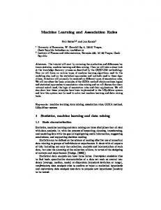
Table 3: MAP Numbers for OHSUMED subset. For all subsets, the best overall results were always obtained by AR (Rqd ). This result is important, since it shows the great value of using query-specific information for sake of ranking. However, this additional information (i.e., query terms) used during model generation, makes unfair a direct comparison of AR (Rqd ) to other methods that do not use this information. So, next we only compare the results obtained by AR (R) and AR (Rd ) to the baseline results. As can be seen in Table 3, all methods showed competitive results in the OHSUMED subset. The worst overall result was obtained by RankBoost (0.440), while the best result was obtained by AR (Rd ) (0.457). The main reason for so much competitiveness is that OHSUMED contains only few features, which are extracted basically from textual evidence, reducing the possibilities of improvements. Still, AR (Rd ) showed improvements (relative to the best baseline, which in this case was ListNet) in 4 trials, while AR (R) showed improvements only in the first two trials. The difference in ranking performance between AR (R) and AR (Rd ) is mainly due to the missing rule problem, which happens when there is not a sufficient number of rules to be applied for some documents in the test set. This problem does not occur with AR (Rd ), which generates rules on a demanddriven basis, according to the need of the document being ranked. Similarly, we believe that other methods may also suffer from insufficient evidence during model generation, explaining the best performance obtained by AR (Rd ). For TD2003, ListNet was again, the most competitive baseline. As shown in Table 4, AR (Rd ) showed improvements in 3 trials, specially in the first one. The overall improvement ranges from 12% (relative to ListNet) to 123% (relative to AdaRank.MAP). In contrast to OHSUMED, TD2003 contains more and diverse features, making possible the achievement of more significant improvements. For TD2004, the most competitive baseline was RankBoost. As shown in Table 5, AR (Rd ) showed improvements in the first three trials, specially in the first one. Again, AR (Rd ) showed the best overall results, with overall improvements ranging from 2.35% (relative to RankBoost) to 31.10% (relative to AdaRank.NDCG). The next set of experiments evaluates the effectiveness of AR (R), AR (Rd ) and AR(Rqd ), in terms of NDCG and precision. Figure 1 shows NDCG and precision numbers obtained from the execution of the evaluated methods. Again, AR (Rqd ) showed to be the best performer, but we will use AR (Rd ) to make a more fair comparison with the baselines. For OHSUMED and TD2004, the results are very competitive, specially in terms of precision. In terms of NDCG,

AR (Rd ) was able to provide a slight overall improvement over the baselines. Again, impressive improvements were obtained using the TD2003 subset. In terms of NDCG, improvements range from 17.30% (relative to Ranking SVM) to 134.61% (relative to AdaRank.NDCG). In terms of precision, improvements range from 15.38% (relative to RankBoost) to 130.67% (relative to AdaRank.NDCG).

5.3 Computational Efficiency The computational efficiency of methods that learn to rank at query-time − AR (Rd ) and AR (Rqd ) − was evaluated through the total execution time, that is, the processing time spent in generating rules and ranking all documents in the test set. The experiments were performed on a Linuxbased PC with a Intel Pentium III 1.0 GHz processor and 1.0 GBytes RAM. Figure 2 (left) depicts the times obtained from the execution of AR (Rd ) for different cache sizes. We varied the cache size from 0 to 150MB, and for each storage capacity we obtained the corresponding execution time. Clearly, execution time is very sensitive to cache size. Caches as large as 150MB are able to store all rules with no need of replacement, being the best configuration. In the OHSUMED subset, times varied from 243 to 11 seconds (corresponding to an average of 0.10 seconds per query). In the TD2003 subset, times varied from 17,504 to 53 seconds (an average of 0.94 seconds per query). But the most impressive result was obtained in the TD2004 subset, where times of AR (Rd ) varied from 38,176 to only 102 seconds (an average of 1.36 seconds per query), an improvement of more than two orders of magnitude, showing that caching is extremely effective, and makes feasible learning to rank at query-time. The reason for the excellent caching performance is depicted in Figure 2 (right), which shows the fraction of documents demanding a specific rule k. For instance, the first rule in the x-axis was demanded for all documents in the test set. That is, the first rule appears in all rule-sets generated by AR (Rd ). Similarly, other rules appear frequently in different rule-sets, indicating that a large fraction of documents in the test set demands rules in common. Since these rules are cached, execution time is greatly reduced. We have shown in Section 5.2 that query terms are valuable for ranking, since the best performance was always obtained by AR (Rqd ). By repeating the previous experiment with varying cache sizes, but now using AR (Rqd ), we also observed that exploring query terms during rule generation does not incur in serious overhead. The increase in execution times varies from only 0.9% (TD2004) to 2.2% (TD2003), when query terms are used during rule generation.

AR Trial R Rd Rqd 1 0.276 (0.18) 0.276 (0.18) 0.293 (0.14) 2 0.289 (0.38) 0.289 (0.38) 0.300 (0.32) 3 0.340 (0.34) 0.340 (0.34) 0.401 (0.30) 4 0.266 (0.89) 0.289 (0.58) 0.324 (0.37) 5 0.222 (0.68) 0.278 (0.35) 0.295 (0.27) Avg 0.291 (0.25) 0.306 (0.07) 0.324 (0.02) Overall Improvements obtained by AR (R) Overall Improvements obtained by AR (Rd ) Overall Improvements obtained by AR (Rqd )

Ranking SVM 0.148 0.270 0.377 0.224 0.263 0.256 13.67% 19.53% 26.56%

RankBoost

FRank

ListNet

0.144 0.257 0.217 0.252 0.191 0.212 37.26% 44.34% 52.83%

0.160 0.299 0.306 0.265 0.195 0.245 18.77% 24.90% 32.24%

0.179 0.271 0.365 0.300 0.250 0.273 6.59% 12.09% 18.68%

AdaRank MAP NDCG 0.205 0.220 0.134 0.134 0.049 0.049 0.189 0.189 0.110 0.333 0.137 0.185 112.41% 57.30% 123.36% 65.40% 136.50% 75.13%

Table 4: MAP Numbers for TD2003 Subset. AR Trial R Rd Rqd 1 0.428 (0.44) 0.495 (0.09) 0.527 (0.07) 2 0.314 (0.67) 0.353 (0.37) 0.378 (0.30) 3 0.374 (0.85) 0.478 (0.26) 0.477 (0.25) 4 0.315 (0.65) 0.315 (0.55) 0.314 (0.68) 5 0.311 (0.82) 0.318 (0.46) 0.319 (0.90) Avg 0.349 (0.04) 0.392 (0.32) 0.403 (0.28) Overall Improvements obtained by AR (R) Overall Improvements obtained by AR (Rd ) Overall Improvements obtained by AR (Rqd )

Ranking SVM 0.410 0.307 0.426 0.252 0.358 0.350 -0.29% 12.00% 15.14%

RankBoost

FRank

ListNet

0.413 0.340 0.440 0.347 0.378 0.383 -8.88% 2.35% 5.22%

0.435 0.363 0.452 0.278 0.376 0.381 -8.40% 2.89% 5.77%

0.403 0.342 0.435 0.321 0.359 0.372 -6.18% 5.37% 8.33%

AdaRank MAP NDCG 0.390 0.391 0.223 0.200 0.407 0.391 0.289 0.260 0.243 0.250 0.331 0.299 5.44% 16.72% 18.43% 31.10% 21.75% 34.78%

Table 5: MAP Numbers for TD2004 Subset. OHSUMED

0.45 0.4

NDCG

0.6 0.5 0.4 0.3

NDCG

0.2 0.7 0.65 0.6 0.55 0.5 0.45 0.4 0.35 0.3

1 0 0 1 0 1 0 1 0 1 0 0 1 01 1 0 1 0 1 0 1 0 1 0 1 0 1 0 1 0 1 0 1 0 1 0 1 01 1 0 0 1 0 1 0 1 0 1 0 1 0 1 0 1 01 1 0 0 1 0 1 0 1 0 1 0 1 0 1 0 1 0 1 0 1 0 1 0 1 0 0 1 01 1 @1

01101010101010 00 11 00 11 00 11 00 11 1010101010101010 00 11 00 11 00 11 0 1 00 11 00 11 1010 101010101010 00 11 00 11

0.6

TD2003

0110 1010 0 1 0 1 0 1 100110 0 1 00 11 0 1 0 00 11 00 11 01 1 00 11 00 11 0 1 0 1 0 1 0 1 00 11 00 11 01 1 0 1 00 11 00 11 011 1 01 1 00 11 011 0 1 00 11 0 1 00 11 00 11 0 1 0 1 0 00 11 00 11 00 0 1 0 1 00 0 1 00 11 0 1 0 00 11 00 11 0 1 0 1 00 11 0 1 00 11 0 1 0 1 00 11 00 11 011 1 01 1 0 1 00 11 0 1 0 1 00 11 00 11 0 1 00 11 0 1 00 11 00 11 0 1 0 1 0 1 00 11 00 11 00 0 1 0 1 0 1 00 01 1 00 11 0 1 011 1 0 1 0 1 00 11 00 11 0 1 0 1 0 00 11 0 1 00 11 0 1 0 1 0 1 00 11 00 11 0 1 0 1 0 1 0 1 00 11 0 1 0 1 011 1 00 11 00 11 0 1 00 0 1 00 11 0 1 00 11 0 1 0 1 00 11 0 1 0 1 00 11 00 11 0 1 00 11 0 1 0 1 0 1 00 11 0 1 00 11 0 1 0 1 0 1 0 1 00 11 00 11 0 1 0 1 0 1 00 11 0 1 00 11 0 1 0 1 0 1 0 1 00 11 00 11 0 1 0 1 0 1 00 11 0 1 00 11 0 1 0 1 0 1 00 11 0011 11 0 1 00 11 0 1 00 11 00 11 0 1 00 11 0 1 0 1 0 1 00 11 0 1 0 1 00 11 00 0 1 00 11 0 1 0 1 0 1 00 11 0 1 00 11 0 1 0 1 0 1 0 1 00 11 00 11 0 1 01011 00 0 1 00 11 0 1 0 1 0 1 01 1 00 11 00 11 0 1 0 1 0 1 1 00 11 01 00 11 0 1 00 11 0 1 00 11 0 1 0 1 0 00 11 0 1 0 1 @2 @4 @5 @3

RankingSVM RankBoost FRank ListNet AdaRank.MAP AdaRank.NDCG

0.7 0.6 0.5 0.4 0.3 0.2

TD2004

1 0 0AR (R) 1 1AR (R,d) 0 1 AR (R,q,d) 0

0110 1001 0 1 0 1 0 1 00 11 10 10 101010 11 1 0 1010 1011 0 1 0 1 00 11 00 00 11 1010 11 0 1 0 1 0 1 00 11 00 11 00 0 1 00 11 0 1 0 1 00 0 1 0 1 00 11 0 1 101010 0 1 0 1 0 1 0 1 00 11 00 11 00 11 00 11 0 1 0 1 0 1 0 1 0 1 0 1 0 1 0 1 00 11 00 11 00 11 0 1 0 1 0 1 00 11 101010101010 11 00 0 1 0 1 10101010 11001011 00 11 10101010 11 101010 11 0 1 0 1 0 1 00 00 11 00 00 11 00 11 0 1 0 1 1010 0 1 0 11 1 00 00 0 1 0 1 00 11 00 11 00 11 0 1 0 1 0 1 0 1 00 11 00 11 00 11 0 1 0 1 00 11 00 11 101011 00 101010101010101011 00 11 00 0 1 0 1 00 11 00 11 00 11 00 00 11 00 11 00 11 0 1 0 1 0 1 0 1 0 1 00 11 0 1 0 1 00 11 00 11 00 11 00 11 0 1 0 1 00 11 00 11 00 11 00 11 0 1 0 1 1010101010101100 11 0 1 0 1 0 1 00 11 0 1 00 11 00 11 0 1 0 1 0 1 0 1 00 11 00 11 0 1 00 11 00 00 0 1 0 1 00 11 00 11 00 11 00 00 00 11 00 11 0 1 0 1 0 1 101010 11 10 00 0 1 0 1 00 00 00 11 00 11 0 1 0 00 11 00 11 00 11 00 11 10 11 01 1 101011 0 1 0 1 00 11 1010 1010 11 00 11 00 11 0 1 10 11 0 11 1 00 11 00 11 1011 00 11 1010101010101011 00 11 00 11 0 1 0 1 00 11 00 00 11 00 11 00 11 00 11 00 11 @5 @2 @3 @4

11 00 00 11 00 11 00 11 00 11 00 11 00 11 0 1 00 11 00 11 0 1 00 11 00 11 0 1 00 11 00 11 0 1 00 11 00 11 0 1 00 11 00 11 0 1 00 11 00 11 0 1 00 11 00 11 0 1 00 11 00 11 0 1 00 11 00 11 0 1 00 11 00 11 0 1 00 11 00 11 0 1 00 11 @1

0.65

0.55

1 0 0AR (R) 1 0AR (R,d) 1 1 AR (R,q,d) 0

0.8 0.7

0110 00 11 00 11 1010101011001010 00 11 0 1 00 11 00 11 1010 1010101010101010 00 11 00 11 00 11

0 1 1 0 0 1 0 1 0 1 0 1 0 1 0 1 0 1 0 1 0 1 0 1 0 1 0 1 0 1 0 1 0 1 0 1 0 1 0 1 0 1 0 1 0 1 0 1 0 1 0 1 0 1 0 1 @2

0.7

Precision

0.5

0011 101010101011001100101010 00 11 00 11 10101010101011001100101010 00 11 1010 00 11 00 11 00 11 001010110010 11

RankingSVM RankBoost FRank ListNet AdaRank.MAP AdaRank.NDCG MHR−BC

RankingSVM RankBoost FRank ListNet AdaRank.MAP AdaRank.NDCG

Precision

NDCG

0.6 0.55

1 0 0 1 0 1 0 1 0 1 0 1 0 1 0 1 0 1 0 1 0 1 0 1 0 1 0 1 0 1 0 1 0 1 0 1 0 1 0 1 0 1 0 1 0 1 0 1 0 1 0 1 0 1 0 1 0 1 0 1 0 1 0 1 0 1 0 1 0 1 @1

0110 1001 101100 1 0 0 1 0 1 1100101011 0 1 0 1 0 1 0 1 00 11 00 0 1 0 1 0 1 00 11 0 1 0 1 0 1 0 1 00 11 0 1 00 11 0 1 0 1 0 1 0 1 00 11 1010 1010 00 11 00 11 00 11 0 1 0 1 0 1 0 1 101011 00 11 0 1 00 0 1 0 1 00 11 0 1 0 1 00 11 0 1 00 11 0 1 0 1 0 1 00 11 0 1 0 1 00 11 00 11 101011 0 1 101011001010 11 0 1 0 1 00 11 00 11 00 11 00 11 00 0 1 0 1 0 1 0 1 0 1 0 1 00 11 0 1 00 11 0 1 0 1 00 11 0 1 0 1 00 11 0 1 00 0 1 00 11 0 1 0 1 0 1 00 11 00 11 0 1 0 1 0 1 00 11 1010 1010101010 00 00 11 00 11 00 1010 101010 11 0 1 0 1 0 1 1011 1011 00 0 1 00 0 1 0 1 00 11 0 1 00 11 001010 11 00 11 00 11 10@311 00 11 @4 @5 10

1 0 0AR (R) 1 0AR (R,d) 1 1 AR (R,q,d) 0

0.75

Precision

0.7 0.65

OHSUMED

1 0 0AR (R) 1 0AR (R,d) 1 1 AR (R,q,d) 0

0.75

0.65 0.6 0.55 0.5 0.45 0.4 0.35 0.3 0.25 0.2

01101010 0 1 0 1 10101011001010 0 1 01 1 0 1 00 1 0 1 101011001010 0 1 0 1 00 11 0 1 0 1 0 1 00 11 0 1 0 1 0 1 01 1 00 11 0 1 0 1 0 0 1 00 11 0 1 1010101100110010101010 0 1 0 1 00 11 0 1 0 1 0 1 0 1 00 11 0 1 0 1 0 1 00 11 0 1 0 1 01010101011001100101010 01 1 00 11 0 1 0 1 0 1 00 11 0 1 0 1 00 11 0 1 0 1 0 1 01 1 00 11 010110010 00 11 @1 0 1 0 1 0 1 0 1 0 1 0 1 0 1 1 0 0 1 0 1 0 1 0 0 1 01 1 0 1 0 1 0 1 0 1 0 1 0 1 0 1 0 1 0 1 0 0 1 01 1 0 1 0 1 0 1 0 1 0 1 0 1 0 1 0 1 0 1 0 1 0 1 0 1 0 1 0 1 0 1 0 1 0 1 01 1 0 0 1 0 1 0 0 1 01 1 0 1 @1

0 1 11 00 1010 1010101010101010 00 11 101010101010 00 11 0 1 00 11 00 11 1010 101010101010 00 11 00 11 00 11 00 11 10 1010101010 00 11

10 0110 10101010 00 11 00 11 1010 10101010101010101010 00 11 00 11 00 11 00 11 1010 10101010101010101010 00 11 00 11 00 11 00 1010 11

1 0 0 1 0 1 0 1 0 1 0 1 0 1 0 1 0 1 0 1 0 1 0 1 0 1 0 1 0 1 0 1 0 1 0 1 0 1 0 1 0 1 0 1 0 1 0 1 0 1 0 1 0 1 0 1 0 1 0 1 0 1 0 1 0 1 @2

0110 1001 101100 1010 10 1 0 00 11 0 1 0 1 110011 00 11 0 1 0 1 0 1 0 1 0 1 00 11 0 1 0 1 00 10101010 1010101011 0 1 101011 00 00 101011 00 11 00 0 1 00 11 0 1 0 1 0 1 00 11 00 11 0 1 00 11 00 11 0 1 00 11 1010 10 0 1 0 1 00 11 00 11 0 1 00 00 11 00 11 0 1 0 1 00 11 011 1 0 1 0 1 0 1 0 1 0 1 0 1 00 11 0 1 00 11 0 1 00 11 00 11 0 1 0 1 0 1 00 11 00 11 0 1 0 1 00 11 0 1 0 1 00 11 0 1 0 1 00 11 00 11 0 1 00 11 0 1 00 11 00 11 00 11 0 1 0 1 00 11 0 1 0 1 0 1 0 1 0 1 0 1 0 1 00 11 0 1 00 11 0 1 00 11 00 001010 11 0 1 00 11 0 1 00 11 0 1 10 1010101010 00 101010 101010 11 0 1 00 00 11 0 1 10@5101011 00 11 00 11 10@311 00 11 @4

RankingSVM RankBoost FRank ListNet AdaRank.MAP AdaRank.NDCG MHR−BC

TD2003

1 0 0AR (R) 1 0AR (R,d) 1 1 AR (R,q,d) 0

0110 0010101010 11 00 11 001010101010101010 11 00 11 0010101010 11

0 01 1 0 1 0 1 0 1 1 0 0 1 0 1 0 1 00 11 0 1 00 11 00 11 0 1 00 11 0 1 00 0 1 00 00 11 0 11 1 00 11 0 1 0 11 1 0011 00 11 11 00 00 11 0 1 00 11 00 11 0 1 00 11 0 1 0 1 00 00 11 00 00 11 0 1 00 11 00 11 0 1 00 11 0 1 0 11 1 0011 11 00 11 00 11 00 11 0 1 00 11 00 11 0 1 00 11 0 1 0 1 00 11 00 11 11 00 11 00 11 0 1 00 00 11 0 1 00 11 0 1 0 1 00 11 00 11 00 11 00 11 0 1 00 11 00 11 0 1 00 11 0 1 0 1 00 11 00 11 00 11 00 11 0 1 00 11 00 11 0 1 00 11 0 1 0 1 00 11 00 11 00 11 00 11 0 1 00 11 00 11 0 1 00 11 0 1 0 1 00 11 00 11 00 11 00 11 01 1 00 00 0 11 00 11 0 1 0 11 1 00 11 00 11 @3 @4 @2 TD2004

10 01 1010 1010101010 00 1010 10101011 00 1010 1011 00 11

0110 1010 1001

RankingSVM RankBoost FRank ListNet AdaRank.MAP AdaRank.NDCG

11 00 00 11 0 1 00 11 0 1 00 0 1 00 11 0 1 00 11 0 1 0 1 1010 1010101011 00 0 1 00 11 0 1 101011 0 1 00 11 00 11 0 1 00 11 00 11 0 1 0 1 0 1 00 11 0 1 00 11 0 1 0 1 0 1 0 1 00 11 00 11 0 1 0 1 0 1 00 11 0 1 00 11 0 1 0 1 0 1 0 1 01 1 00 0 1010 101011 0 1 00 11 00 11 1@5 0 10 1 0 0AR (R) 1 1AR (R,d) 0 1 AR (R,q,d) 0

1010 1001 0 1 1 0 00 0 1 10101010 00 11 0 1 0 1 00 11 10101010 11 00 11 00 11 0 1 0 1 10 00 0 1 010 00 11 10101010101010 11 1 0 0 1 00 11 0 1 1 00 11 0 1 0 1 10101011 1010 11 00 11 0 1 00 11 00 11 0 1 00 11 0 1 0 1 00 0 1 0 1 00 11 0 1 00 11 00 11 0 1 0 1 00 0 1 00 11 0 1 0 1 0 1 0 1 00 11 0 1 00 11 10101010 0 1 00 11 0 1 0 1 00 11 0 1 00 11 0 1 0 1 00 11 1010101010101010 11 1010 11 0 1 0 1 00 11 0 1 1010 11 00 11 0 1 00 00 11 00 11 10 11 0 1 0 1 00 11 101011 0 1 00 0 1 00 11 0 1 0 1 00 0 1 00 0 1 00 11 0 1 0 1 0 1 00 11 0 1 00 11 00 11 0 1 00 0 1 00 11 0 1 00 11 0 1 0 1 00 11 00 11 0 1 0 1 0 11 1 00 11 00 11 0 1 00 11 00 11 0 1 00 11 00 11 00 11 0 1 00 11 0 1 00 11 0 1 0 1 00 11 0 1 0 1 00 11 0 1 00 11 00 0 1 0 1 00 11 00 11 01 1 1010 00 11 0 1 00 11 0 1 101011 10101011 00 11 0 1 00 11 00 11 0 1 00 11 00 11 0 1 00 0 0 1 00 00 11 1010101010101010 11 0 1 0 1 0 1 00 00 11 0 1 0 1 00 11 00 11 0 1 00 11 00 11 00 11 0 1 00 11 0 1 00 11 0 1 00 11 0 1 0 1 00 11 0 1 00 11 00 11 0 1 0 1 00 11 00 11 0 1 00 11 0 1 0011 11 0 1 101011 00 11 0 1 00 11 00 11 0 1 00 11 011 1 00 11 0 1 00 0 00 00 11 1010 10 11 0 1 0 1 00 00 01 1 0 1 00 11 00 11 0 1 00 11 00 11 00 11 0 1 0 1 0 1 00 11 00 11 0 1 @2 @3 @4 @5

11 00 00 11 00 11 00 11 00 11 00 11 00 11 00 11 0 1 00 11 00 11 0 1 00 11 00 11 0 1 00 11 00 11 0 1 00 11 00 11 0 1 00 11 00 11 0 1 00 11 00 11 0 1 00 11 00 11 0 1 00 11 00 11 0 1 00 11 00 11 0 1 00 11 00 11 0 1 00 11 00 11 0 1 00 11 00 11 0 1 00 11 00 11 0 1 00 11 00 11 0 1 00 11 00 11 0 1 @1

RankingSVM RankBoost FRank ListNet AdaRank.MAP AdaRank.NDCG

Figure 1: NDCG and Precision Numbers for OHSUMED, TD2003 and TD2004 Subsets.

OHSUMED TD2003 TD2004

10000

1000

100

10 0

20 40 60 80 100 120 140 Cache Size (MB)

1 Fraction of Documents

Execution Time (sec)

100000

0.1 0.01 0.001 0.0001 OHSUMED TD2003 TD2004 1e−05 1 10

100

1000

10000 100000

k

Figure 2: Left − Effect of Caching in Exec. Time. Right − Fraction of Documents demanding Rule k.

6.

CONCLUSIONS AND FUTURE WORK

In this paper we propose and evaluate novel methods that learn to rank. The proposed methods introduce interesting innovations, such as the use of association rules and the ability to learn ranking models at query-time (enabling the better use of more discriminative information, such as query terms). By generating rules on a demand-driven basis, depending on the documents to be ranked, only the necessary information is extracted from the training data, resulting in fast and effective ranking methods. Experimental results, obtained using the LETOR benchmark, indicate that methods that learn to rank at query-time outperform the state-ofthe-art methods. The results also suggest that query terms are valuable information for sake of ranking. The running times of the proposed methods, which are able to rank a document in roughly 0.0007 seconds, is also worth mentioning, and makes feasible learning ranking models at query-time. As future work, we intend to improve performance in two directions: (i) by combining the results obtained by multiple methods, and (ii) by exploring other query-specific information, such as query type (navigational, transactional etc.).

7.

REFERENCES

[1] R. Agrawal, T. Imielinski, and A. Swami. Mining association rules between sets of items in large databases. In Proc. of the SIGMOD Conf., pages 207–216. ACM, 1993. [2] H. Almeida, M. Gon¸calves, M. Cristo, and P. Calado. A combined component approach for finding collection-adapted ranking functions based on genetic programming. In Proc. of the SIGIR Conf., pages 399–406. ACM, 2007. [3] R. Baeza-Yates and B. R-Neto. Modern Information Retrieval. Addison-Wesley-Longman, 1999. [4] C. Burges, T. Shaked, E. Renshaw, A. Lazier, M. Deeds, N. Hamilton, and G. Hullender. Learning to rank using gradient descent. In Proc. of the ICML, pages 89–96. ACM, 2005. [5] Y. Cao, J. Xu, T. Liu, H. Li, Y. Huang, and H. Hon. Adapting ranking SVM to document retrieval. In Proc. of the SIGIR Conf., pages 186–193. ACM, 2006. [6] Z. Cao, T. Qin, T. Liu, M. Tsai, and H. Li. Learning to rank: from pairwise approach to listwise approach. In Proc. of the ICML, pages 129–136. ACM, 2007. [7] K. Crammer and Y. Singer. A new family of online algorithms for category ranking. In Proc. of the SIGIR Conf., pages 151–158. ACM, 2002.

[8] W. Fan, M. Gordon, and P. Pathak. Personalization of search engine services for effective retrieval and knowledge management. In Proc. of the ICIS, pages 20–34, 2000. [9] W. Fan, M. Gordon, and P. Pathak. Discovery of context-specific ranking functions for effective information retrieval using genetic programming. TKDE, 16(4):523–527, 2004. [10] W. Fan, M. Gordon, and P. Pathak. Genetic programming-based discovery of ranking functions for effective web search. J. of Management Information Systems, 21(4):37–56, 2005. [11] U. Fayyad and K. Irani. Multi interval discretization of continuous-valued attributes for classification learning. In In Proc. of the IJCAI., pages 1022–1027. Morgan Kaufmann, 1993. [12] Y. Freund, R. Iyer, R. Schapire, and Y. Singer. An efficient boosting algorithm for combining preferences. J. of Machine Learning Research, 4:933–969, 2003. [13] J. Gao, H. Qi, X. Xia, and J. Nie. Linear discriminant model for information retrieval. In Proc. of the SIGIR Conf., pages 290–297. ACM, 2005. [14] R. Herbrich, T. Graepel, and K. Obermayer. Large margin rank boundaries for ordinal regression. MIT Press, 2000. [15] T. Joachims. Optimizing search engines using clickthrough data. In Proc. of the KDD Conf., pages 133–142. ACM, 2002. [16] J. Koza. Genetic Programming: On the programming of computers by natural selection. MIT Press, 1992. [17] B. Liu, W. Hsu, and Y. Ma. Integrating classification and association rule mining. In Proc. of the KDD Conf., pages 80–86. ACM, 1998. [18] Y. Liu, J. Xu, T. Qin, W. Xiong, and H. Li. LETOR: Benchmark dataset for research on learning to rank for information retrieval. In Proc. of the Learning to Rank Workshop in conjuntion with SIGIR, 2007. [19] T. Mitchell. Machine Learning. McGraw Hill, 1997. [20] R. Nallapati. Discriminative models for information retrieval. In Proc. of the SIGIR Conf., pages 64–71. ACM, 2004. [21] T. Qin, X. Zhang, D. Wang, T. Liu, W. Lai, and H. Li. Ranking with multiple hyperplanes. In Proc. of the SIGIR Conf., pages 279–286. ACM, 2007. [22] A. Trotman. Learning to rank. Information Retrieval, 8(3):359–381, 2005. [23] M. Tsai, T. Liu, T. Qin, H. Chen, and W. Ma. FRank: a ranking method with fidelity loss. In Proc of the SIGIR Conf., pages 383–390. ACM, 2007. [24] J. Xu and H. Li. Adarank: a boosting algorithm for information retrieval. In Proc. of the SIGIR Conf., pages 391–398. ACM, 2007. [25] Y. Yue, T. Finley, F. Radlinski, and T. Joachims. A support vector method for optimizing average precision. In Proc. of the SIGIR Conf., pages 271–278. ACM, 2007. [26] M. Zaki, S. Parthasarathy, M. Ogihara, and W. Li. New algorithms for fast discovery of association rules. In Proc. of the KDD Conf., pages 283–296, 1997. [27] J. Zobel and A. Moffat. Exploring the similarity space. SIGIR Forum, 32(1):453–490, 1998.