Institut für Geodäsie und. Photogrammetrie an der Eidgenössischen. Technischen Hochschule. Zürich. Mitteilungen Nr. 92. Least Squares 3D Surface Matching.
Institut für Geodäsie und Photogrammetrie an der Eidgenössischen Technischen Hochschule Zürich Mitteilungen Nr.
92 Least Squares 3D Surface Matching
Devrim Akca
Zürich, 2007
This publication is an edited version of: __________________________________________________________________________________ Diss. ETH No. 17136
Least Squares 3D Surface Matching A dissertation submitted to the SWISS FEDERAL INSTITUTE OF TECHNOLOGY ZURICH for the degree of Doctor of Sciences presented by DEVRIM AKCA M.Sc., Karadeniz Technical University born 27th of May, 1975 citizen of Turkey accepted on the recommendation of Prof. Dr. Armin Grün, examiner ETH Zurich, Switzerland Prof. Dr. Orhan Altan, co-examiner Istanbul Technical University, Turkey Zurich 2007 __________________________________________________________________________________ IGP Mitteilung Nr. 92 Least Squares 3D Surface Matching Devrim Akca March 2007 Copyright © 2007, Devrim Akca All rights reserved Published by Institut für Geodäsie und Photogrammetrie Eidgenössische Technische Hochschule Zürich ETH Hönggerberg CH-8093 Zürich ISSN 0252-9335 ISBN 3-906467-63-5
To the wishes of my mother… (1950-1983)
FOREWORD Nowadays we dispose of various sensors and automated methods to produce large quantities of point clouds in a relatively short time. Very often an object is built up by a number of point cloud patches, which refer to different datums. Therefore the issue of co-registration of point clouds, representing 3D surfaces, is a serious topic in 3D modeling. Traditionally, some of the system manufacturers suggest to use specific tie points to be put into the scene for co-registration – a very tedious and not so accurate procedure. Progress was achieved with the ICP (Iterative Closest Point) technique, which uses only intrinsic surface information for co-registration. However, the ICP technique has a number of disadvantages, as described in this thesis, which the new method proposed here- 3D Least Squares Surface Matching- has overcome. 3D LS Surface Matching is a generalization of 2D LS image matching and has the same underlying ideas and concepts. In this context it is a generalization, like the previously developed 3D voxel cube matching and the line feature extraction techniques, both based on Least Squares Matching. The author of this thesis has developed this technique, both in terms of theoretical penetration, practical and efficient computer implementation and has shown in quite a number of different application cases the power of this method. The proposed method estimates the transformation parameters of one or more fully 3D search surfaces with respect to a template one, using the Generalized Gauss-Markoff model, minimizing the sum of squares of the Euclidean distances between the surfaces. It fully considers 3D geometry. The geometric relationship between the conjugate surface patches is defined as a 7-parameter 3D similarity transformation. This parameter space can be extended or reduced, as the situation demands. In case of lack of sufficient geometric information the procedure may fail, e.g. in case of matching of two planes or spherical and cylindrical objects. An object surface may have some attribute information attached to it. Intensity and color are well known examples. Devrim Akca proposed an extension that can simultaneously match intensity information and geometry under a combined estimation model. The mathematical model is flexible. Further conceptual extensions are given, as the Least Squares matching of 3D curves and matching of 3D curves or 3D sparse point clouds (e.g. ground control points) with a 3D surface. Additionally, a general framework for the simultaneous matching and georeferencing of multiple 3D surfaces with their intensity information has been formulated and will be further developed in the near future. As evidenced by the many projects shown in this thesis the method works fine under a great variety of different conditions (use of satellite, aerial and terrestrial images, structured light systems, laserscanners, very dense and sparse point clouds, integrated image intensity data, simultaneous georeferencing and multi-patch matching). The method of Multi-Patch 3D Least Squares Surface and Intensity Matching is a very substantial contribution of photogrammetry to the very broad and general problem of 3D Modeling. Devrim Akca has researched, tested and applied this technique in an exemplary and excellent way. During all the time of hard and diligent work, which also included some other, smaller R&D projects, Devrim has never lost his ambitions and always showed great optimism and dedication. He was always a competent, friendly and solidary team-player. For all this I would like to congratulate him very much! It is to be expected that this work will serve as a valuable reference for all experts concerned with 3D modeling for quite some years to come. Zurich, May 2007
Prof. Dr. Armin Gruen
ABSTRACT Laser scanners can measure directly 3D coordinates of huge amounts of points in a short time period. Most of them also provide an intensity value for every point. This abundant data can be efficiently used to model the scene. In many cases, the object has to be scanned from different viewpoints in order to completely reconstruct it. Because each scan has its own local coordinate system, all the different pointclouds must be transformed into a common system. This procedure is usually referred to as co-registration. Actually, the co-registration is not a problem specific to the laser scanner domain. Also in photogrammetry, we face many similar problems. The automatic co-registration of pointclouds, representing 3D surfaces, is a relevant problem in 3D modeling. This multiple registration problem can be defined as a surface matching task. In photogrammetry, surface matching was first touched by Gruen (1985a) as a straight extension of the Least Squares image matching. This thesis work gives a generalization of this 2D technique to the 3D surface matching problem. The proposed method estimates the transformation parameters of one or more fully 3D search surfaces with respect to a template one, using the Generalized Gauss-Markoff model, minimizing the sum of squares of the Euclidean distances between the surfaces. It fully considers 3D geometry. An observation equation is written for each surface element on the template surface patch, i.e. for each sampled point. Each equation functionally relates the observations of the template to the parameters of search surface. The constant term of the adjustment is given by the observation vector whose elements are the Euclidean distances between the template and search surface elements. The matching is achieved by Least Squares minimization of a goal function, which measures the Euclidean distances between the surfaces. The final location of the search surface is estimated with respect to an initial state. The geometric relationship between the conjugate surface patches is defined as a 7-parameter 3D similarity transformation. This parameter space can be extended or reduced, as the situation demands it. Since the functional model is non-linear, the system is linearized by Taylor expansion. The numerical derivative terms are defined as surface normals. The unknown transformation parameters are treated as stochastic quantities using proper a priori weights. This extension of the mathematical model gives control over the estimation parameters. The solution is iterative. After the joint system is solved, the search surface is transformed to a new state using the updated set of transformation parameters, and the design matrix and the discrepancies vector are re-evaluated. The iteration stops if each element of the alteration vector falls below a certain limit. Besides the mathematical model of the procedure, a comprehensive discussion is given about the implementation details, precision and reliability issues, and convergence behavior. Special attention is paid to the computational aspects. Two strategies in order to decrease the computation time were implemented. The main portion of the computational complexity is to search the correspondent elements between the surfaces, whereas the adjustment part is a small system, and is quickly solved using Cholesky decomposition followed by back-substitution. A rapid space partitioning method is given for searching the correspondences. It is a 3D boxing structure combined with a hierarchical local and adaptive nearest neighborhood search. The local neighborhood is hierarchically updated during the iteration. The second acceleration strategy is simultaneous matching of sub-surface patches, which are selected in cooperative surface areas. They are joined to the system by the same 3D transformation parameters. The individual patches may not include sufficient information for the matching of whole surfaces, but together they provide a computationally effective solution, since they consist of only relevant information rather than using the full data set. In case of lack of sufficient geometric information the procedure may fail, e.g. in case of matching of two planes or spherical objects. An object surface may have some attribute information attached to it. Temperature, intensity, and color are well known examples. Most of the laser scanners can supply intensity information in addition to Cartesian coordinates for each point. We propose an extension that
vii
can simultaneously match intensity information and geometry under a combined estimation model. In this approach the intensity image of the pointcloud also contributes observation equations to the system, considering the intensities as supplementary information to the range image. The mathematical model is flexible. Further conceptual extensions are given as the Least Squares matching of 3D curves and matching of 3D curves or 3D sparse points (e.g. ground control points) with a 3D surface. Additionally, a general framework for the simultaneous matching and georeferencing of multiple 3D surfaces with their intensity information is formulated. The method derives its mathematical strength from the Least Squares matching concept and offers a high level of flexibility for many kinds of 3D surface correspondence problems. The experiments demonstrate the capabilities of the basic method and the extensions.
viii
ZUSAMMENFASSUNG Laserscanning ermöglicht die direkte Bestimmung einer grossen Anzahl von 3D Koordinaten in kurzer Zeit, zusätzlich liefern viele dieser Systeme einen Intensitätswert zu jedem gemessenen Punkt. Die so erzeugte Fülle von Informationen wird genutzt, um den aufgenommenen Raum effizient zu modellieren. Für eine vollständige Rekonstruktion des erfassten Raums ist es notwendig, das zu erfassende Objekt von unterschiedlichen Standpunkten aus aufzunehmen. Da jeder Scan in einem eigenen Koordinatensystem vorliegt, ist es notwendig, alle erfassten Punktwolken in ein einheitliches System zu überführen. Dieser Vorgang wird als Co-Registrierung bezeichnet. Dies ist jedoch keine spezifisches Fall des Laserscannings, auch in der Photogrammetrie steht man diesem Problem in vielen Fällen gegenüber. Die automatische Co-Registrierung von Punktwolken, welche 3D Flächen repräsentieren, ist eine wichtige Aufgabenstellung im Zuge der Modellierung. Dieses Problem der Mehrfachregistrierung kann als Surface-Matching Problem behandelt werden. Im Rahmen der Photogrammetrie wurde diese Aufgabe zum ersten Mal von Grün (1985a), als direkte Erweiterung des Least-Squares Image Matching erwähnt. Die hier präsentierte Arbeit befasst sich mit der Erweiterung dieses zweidimensionalen Ansatzes, hin zu einem Matchingverfahren dreidimensionaler Flächen. Die hier vorgestellte Methode bestimmt die Transformationsparameter einer oder mehrerer dreidimensionaler Flächen bezüglich einer Referenzfläche (Template), unter Verwendung des allgemeinen Gauss-Markoff Modells, welchem die Minimierung der Summe der Quadrate, des euklidischen Abstandes zwischen den Flächen zugrunde legt. Hierbei wird vollumfänglich die dreidimensionale Information des Objektes berücksichtigt. Für jedes Element der Referenzfläche, z.B. für jeden Punkt, ergibt sich eine Beobachtungsgleichung. Jede dieser Gleichungen beschreibt den Zusammenhang zwischen Beobachtungen der Referenzfläche und den Transformationsparametern der anzupassenden Fläche (Search-Surface). Das Absolutglied der Ausgleichung ist durch den Beobachtungsvektor gegeben, dessen Elemente den euklidischen Distanzen zwischen den Elementen der Referenzfläche und denen der anzupassender Fläche entsprechen. Das Matching wird mittels Minimierung der Zielfunktion nach kleinsten Quadraten durchgeführt, welches die euklidischen Distanzen zwischen den Oberflächen beschreibt. Die Endposition der anzupassenden Fläche wird bezüglich eines Startwertes bestimmt. Der geometrische Zusammenhang zwischen konjugierten Flächen wird mittels einer 7-Parameter Ähnlichkeitstransformation beschrieben. Dieser Parameterraum kann je nach Anforderung erweitert oder reduziert werden. Das verwendete funktionale Modell ist nichtlinear, somit ist eine Linearisierung nach Taylor notwendig. Die numerisch abgeleiteten Terme sind als Flächennormale definiert. Die unbekannten Transformationsparameter werden als stochastische Grössen mit geeigneter Gewichtung beschrieben. Diese Erweiterung des mathematischen Modells ermöglicht eine bessere Kontrolle über die zu bestimmenden Parameter. Die Bestimmung der Parameter erfolgt iterativ. Nach jeder Lösung des Systems wird die anzupassende Fläche, mittels der bestimmten Parameter, in ihre neue Lage transformiert und die Designmatrix sowie der Vektor der Verbesserungen neu bestimmt. Dieser Iterationsvorgang wird beendet, wenn jedes Element des Unbekanntenvektors einen bestimmten Grenzwert unterschreitet. Neben dem mathematischen Modell werden Details der Implementation, Präzision, Zuverlässigkeit und des Konvergenzverhaltens ausführlich diskutiert. Besonderes Augenmerk wird hier auf rechentechnische Aspekte gelegt. Um eine Reduktion der Rechenzeit zu erzielen, wurden zwei verschiedene Berechnungsverfahren implementiert. Der grösste Teil des Rechenaufwandes wird für die Suche nach korrespondierenden Elementen zwischen den Oberflächen verwendet, wohingegen die Ausgleichung selbst nur den kleineren Teil einnimmt. Die Ausgleichung wurde mittels Cholesky Algorithmus sehr effizient gelöst. Zum Auffinden der korrespondierenden Oberflächenelemente wurde eine effiziente Unterteilung des Objektraumes durchgeführt. Diese basiert auf einer 3D-Box Struktur
ix
mit hierarchischer lokalen und adaptiver Nearest Neighborhood Suche. Die lokalen Nachbarschaften werden während der Iteration hierarchisch aktualisiert. Eine weitere Möglichkeit besteht darin, lediglich Teile des Überlappungsbereichs zu nutzen, wobei diese Teile aus kooperativen Teilen des Gesamtmodells stammen. Diese einzelnen Unterteile enthalten unter Umständen nicht genügend Informationen um die gesamten Flächen zu registrieren, jedoch ergibt sich aus der Kombination der einzelnen Lösungen eine korrekte und effektive Lösung des Problems, da die Teilflächen nur relevante Informationen im Gegensatz zur gesamten vorhandenen Fläche aufweisen. Im Fall fehlender geometrischer Information ist jedoch ein Fehlschlagen des Algorithmus möglich, z.B. beim Matching zweier Ebenen oder Kugeln. Einer Oberfläche kann zusätzliche Informationen enthalten. Temperatur, Intensität und Farbe sind einige der bekanntesten. Die meisten Laserscanner können Intensitätsinformationen bezüglich eines kartesischen Koordinatensystems für jeden gemessenen Punkt zur Verfügung stellen. Wir erweiterten unseren Ansatz, hin zu einer simultanen Auswertung von Intensitätsinformationen und Geometrie, in einem kombinierten mathematischen Modell. Bei diesem Ansatz tragen die Intensitätsbilder, als zusätzliche Information neben den eigentlichen Daten aus dem Laserscanning, weitere Beobachtungsgleichungen zur Ausgleichung bei. Das vorgestellte mathematische Modell ist flexibel. Konzeptionelle Erweiterungen, wie das LeastSquares Matching von 3D Kurven, sowie das Matching von 3D Kurven oder 3D Punkten (z.B. Passpunkten) bezüglich einer 3D Oberfläche werden erläutert. Zusätzlich wurde das Grundgerüst für simultanes matching und georeferenzieren von mehreren 3D Oberflächen unter Nutzung von Intensitätsinformationen formuliert. Die dargestellte Methodik erhält ihre mathematische Strenge durch die Ausgleichung nach kleinsten Quadraten und weist eine hohe Flexibilität zur Anwendung auf viele Arten von dreidimensionalen Flächenkorrespondenzproblemen auf. Die aufgezeigten Beispiele spiegeln die Möglichkeiten der grundlegenden Methode und der Erweiterungen wieder.
x
TABLE OF CONTENTS 1. Introduction ……………………………………………………………………....…….………. 1 1.1. Motivation …………………………………………………………………….…….……….. 1 1.2. Research aim …………………………………………………………………….…….…….. 1 1.3. Overview of the thesis contents ………………………………………………….…...…..…. 2 2. Review of previous work on surface matching ………………………………….......….....….. 5 2.1. Early work on surface matching …………………………………………………....….……. 5 2.2. Related work on acceleration strategies …………………………………………........…….. 6 2.3. Related work on multiple surface matching …………………………………...............……. 7 2.4. Related work in terrain modeling ……………………………….…………………….…….. 8 2.5. Related work on combined matching of geometry and intensity ………….......…….....…… 9 2.6. Related work on curve matching ……………………...………….…………………………. 9 3. Least squares 3D surface matching ………………………………….……………….……….. 11 3.1. The basic estimation model ……………………………………………………….………… 11 3.2. Surface representation and numerical derivatives …………………………….…….………. 14 3.3. Numerical derivatives on the template surface ………………………………………...……. 15 3.4. Precision, reliability and error detection ………………………………………………..…… 16 3.5. Convergence behavior …………………………………………………………….………… 16 3.6. Computational aspects ………………………………………………………….…………… 16 3.7. The Generalized Gauss-Markoff versus Levenberg-Marquardt …………………..………… 17 3.8. Acceleration strategies ……………………………………………………………….……… 17 3.8.1. Fast correspondence search with boxing structure ………………………...………….. 17 3.8.2. Simultaneous multi-subpatch matching ………………………………….…...………. 19 3.9. Multiple surface matching ………………………………………………….………..……… 20 4. Simultaneous matching of surface geometry and intensity ……………………..…………… 21 4.1. Formation of quasisurfaces …………………………………………………….….………… 21 4.2. Estimation model ………………………………………………………………...………….. 22 5. Further conceptual extensions …………………………………….…………………..………. 25 5.1. Least squares 3D curve matching ………………………………….……………….……….. 25 5.2. Matching of 3D curves with a 3D surface …………………………….………….…………. 27 5.3. Matching of 3D sparse points with a 3D surface ……………………..………………..……. 27 5.4. Generalized multiple 3D surface and intensity matching ……………………………..……. 27 5.4.1. Least squares multiple 3D surface matching …………………………………….…… 28 5.4.2. The generalized model with intensity matching and georeferencing ………………… 29 6. Experimental results ……………………………………………………….…………...……… 31 6.1. Experiments for the basic algorithm ……………………………………….…………...…… 31 6.1.1. Human face …………………………………………………………….……….…….. 31 6.1.2. Industrial plant ………………………………………………………….......………… 32 6.1.3. Newspaper …………………………………………….…………………….………… 33 6.1.4. Tucume …………………………………………………..………………………...….. 35 6.1.5. Bas-relief ……………………………………………………………………………… 36 6.2. Experiments for the simultaneous matching of surface geometry and intensity ……….…… 37 6.2.1. Ball ………………………………………………………………………….………… 37 6.2.2. Wall painting ……………………………………………………………….…………. 38 6.3. Diverse applications ……………………………………………………………..……...…… 39 6.3.1. Chapel – 3D object modeling …………………………………………….........……… 39 xi
6.3.2. Weary Herakles – cultural heritage ………………………………………........……… 41 6.3.2.1. The story ………………………………………………………........………… 41 6.3.2.2. Data acquisition in the Antalya Museum ……………………….……………. 42 6.3.2.3. Pointcloud registration …………………………………………….….……… 42 6.3.2.4. Surface modeling and texture mapping …………………………….…...……. 42 6.3.3. Khmer head – cultural heritage ………………………………………..………...……. 43 6.3.3.1. Data acquisition in Museum Rietberg …………………………...……..…….. 43 6.3.3.2. Pointcloud registration ……………………………………..…………..…….. 44 6.3.3.3. Surface modeling …………………………………….......……………..…….. 44 6.3.3.4. Texture mapping ………………………………………………………..…….. 46 6.3.4. Pinchango Alto – terrain modeling …………………………………………...………. 47 6.3.4.1. The scanning campaign ………………………………………………....……. 47 6.3.4.2. Pairwise registration with the LS3D surface matcher …………….…….……. 48 6.3.4.3. Global registration ………………………………………………........………. 50 6.3.4.4. Surface modeling ……………………………………………………..………. 51 6.3.5. SRTM TerrainScape™ - filling the holes of SRTM C-Band DEMs ………..…….….. 51 6.3.6. Accuracy evaluation of DSMs derived from DMC digital airborne camera …........…. 52 6.3.6.1. Image and LIDAR data ……………………………………………..….…….. 52 6.3.6.2. Aerial triangulation and DSM generation ………………………........………. 52 6.3.6.3. DSM results and analysis ……………………………………………..……… 53 6.3.7. Assessing change of forest area and shrub encroachment ……………………………. 56 6.3.7.1. Study area and data sets ………………………………………………………. 56 6.3.7.2. Co-registration and change detection ………………………………………… 57 6.3.8. Accuracy assessment of the SRTM C-Band DEMs …………………………………... 60 6.3.8.1. Reference DEM – Hobart …………………………………………………….. 60 6.3.8.2. SRTM C-Band DEM – Hobart ……......……………………………………… 61 6.3.8.3. Quantitative results of Hobart test site ……..………………………………… 61 6.3.8.4. Cross-comparison of the SRTM C- and X-Band DEMs – Neuschwanstein …. 62 7. Conclusions and Outlook ……………………………………………………….......…………. 65 7.1. Summary ………………………………………………………………………….…………. 65 7.2. Conclusions ……………………………………………………………………..……..…….. 66 7.3. Outlook ………………………………………………………………………………...……. 67 Bibliography …………………………………………………………………………….………… 69 Acknowledgements ………………………………………………………………………..……… 77 Curriculum Vitae ……………………………………………………………………….……..….. 78
xii
LIST OF FIGURES Figure 1. Figure 2. Figure 3. Figure 4. Figure 5. Figure 6. Figure 7. Figure 8. Figure 9. Figure 10. Figure 11. Figure 12. Figure 13. Figure 14. Figure 15. Figure 16. Figure 17. Figure 18. Figure 19. Figure 20. Figure 21. Figure 22. Figure 23. Figure 24. Figure 25. Figure 26. Figure 27. Figure 28. Figure 29. Figure 30. Figure 31. Figure 32. Figure 33. Figure 34. Figure 35.
Representation of surface elements in planar and bi-linear forms ………………… 14 Typical examples for fast and slow convergence ………………………………..... 17 3D Boxing structure …………………….…………………………………...…….. 18 Forming the quasisurface ………………………………………………….………. 21 Matching of free-form space curves ………………………….…………………… 25 Local affine system and Frenet frame ………………………………………….….. 26 Matching of a 3D space curve with a 3D surface ……………………………...….. 27 Experiment “human face” ……………………………………………………...….. 32 Experiment “industrial plant” ………………………...………………………..….. 33 Experiment “newspaper” ………………………………………………………….. 34 Experiment “Tucume” …………………………………………………………….. 36 Experiment “bas-relief” …………………………………………………………… 37 Experiment “ball” …………………………………………………………..……… 38 Experiment “wall painting” …………………………………………………….….. 39 The final result of “chapel” experiment ………………………….…………….….. 40 Weary Herakles statue ……………………………………………………...……… 41 3D model of the Weary Herakles statue ……………………………………..……. 43 The Khmer head in the Museum Rietberg ………………………………………… 44 Shaded view of the Geomagic Studio and PolyWorks models ……………………. 45 The illumination system used for the texture mapping ………………………...….. 46 Texture mapped 3D model of the Khmer head …………………………….……… 47 Day by day scan coverage of Pinchango Alto …………………………………….. 48 Large occlusion areas in Pinchango Alto …………………………………..……… 48 3D model of Pinchango Alto …………………………………………………...….. 50 Filling the data holes of SRTM C-Band DEMs …………………………………… 51 The 1m grid matching DSM using ACX orientation …………………………..….. 53 Residuals (3D spatial differences between master and slave DSMs) for PAT-B and ACX orientations ………………………………………………..………..…… 55 Color coded DSMs generated by use of SAT-PP software …………………..……. 57 The Z components of the Euclidean distances between 1997 and 2002 matching DSMs ……………………………………………………………………………… 58 The Euclidean distances between 2001 LIDAR DSM and 2002 matching DSM .... 59 The reference IKONOS DEM and its corresponding SRTM C-Band DEM ……… 60 The data conversion pipeline for the C-Band DEM ……………………………….. 61 Colored spatial (distance) discrepancies between the reference and C-Band DEMs of Hobart test site ………………………………………………………………….. 62 SRTM X-Band DEM of the Neuschwanstein area and its C-Band DEM counterpart …………………………………………………………………………. 63 Cross-comparison between the X- and C-Band DEMs at the test site Neuschwanstein ……………………………………………………………………. 64
xiii
LIST OF TABLES Table 1. Table 2. Table 3. Table 4. Table 5. Table 6. Table 7. Table 8. Table 9. Table 10. Table 11. Table 12. Table 13. Table 14. Table 15. Table 16.
The iteration criteria values for the elements of the translation vector and the rotation angles ………………………………………………………………..……. 31 Numerical results of “human face” experiment …………………………………… 32 Numerical results of “industrial plant” experiment ……………………......……… 32 Numerical results of “newspaper” experiment …………………………….……… 35 Numerical results of “Tucume” experiment ………………………………………. 35 Numerical results of “bas-relief” experiment ……………..………………………. 36 Numerical results of “ball” example ………………………………………………. 38 Numerical results of “wall painting” example ………………………...……….….. 39 Numerical results of “chapel” experiment ………………………………........…… 41 Numerical results of the LS3D matchings in “Pinchango Alto” experiment ……… 49 The results of the LS3D program in DMC experiment …………………….……… 54 Decomposition of values of Table 10 in X, Y and Z components in DMC experiment ……………………………………………………………………...….. 54 Characteristics of the CIR-aerial images ……………………….………………….. 56 Technical details of the reference DEM of Hobart ………………………………... 60 Numerical results of the analysis of the C-Band DEM in the test site Hobart …….. 61 Numerical results of the cross-comparison of the X- and C-Band DEMs in the test site Neuschwanstein ……………………………………………………………….. 63
xiv
1.1. Motivation
1 INTRODUCTION 1.1. Motivation For 3D object modeling data acquisition must be performed from different standpoints. The derived local pointclouds (or surfaces) must be transformed into a common coordinate system. This procedure is usually referred to as co-registration. In practice special targets, provided by the terrestrial laserscanning vendors (e.g. Zoller+Fröhlich, Leica, Riegl), are mostly used for co-registration of pointclouds. However, such a strategy has several deficiencies with respect to fieldwork time, personnel and equipment costs, and accuracy. In a recent study, Sternberg et al. (2004) reported that registration and geodetic measurement parts comprise 1020% of the whole project time. In another study, a collapsed 1000-car parking garage was documented in order to assess the damage and structural soundness of the structure. The scanning took 3 days, while the conventional survey of the control points required 2 days (Greaves, 2005). In our work at Pinchango Alto (details given in Chapter 6.3.3), two persons set the targets to the field and measured with RTK-GPS in 1½ days. Not only fieldwork time but also accuracy is another important concern. The target based registration methods cannot exploit the full accuracy potential of the data. The geodetic measurement naturally introduces some error, which might exceed the internal error of the scanner instrument. In addition, the targets must be kept stable during the whole scanning campaign. This might be inconvenient with the scanning works stretching over more than one day. Surface based registration techniques stand as efficient and versatile alternative to the target based techniques. They simply bring the strenuous additional fieldwork of the registration task to the computer in the office while optimizing the project cost and duration and achieving a better accuracy. In the last decade, the surface based registration techniques have been studied extensively. It is still an active research area. An exhaustive literature review, which gives a large number of research activities on the topic, given in the next chapter, demonstrates the relevance of the problem. Co-registration is crucially needed wherever spatially related data sets can be described as surfaces and have to be transformed to each other. Examples can be given in medicine, computer graphics, animation, cartography, virtual reality, industrial inspection and quality control, spatial data fusion, cultural heritage, photogrammetry, etc.
1.2. Research aims The Least Squares matching (LSM) concept had been developed in parallel by Gruen (1984; 1985a), Ackermann (1984) and Pertl (1984). It has been applied to many different types of measurement and feature extraction problems due to its high level of flexibility and its powerful mathematical model: adaptive Least Squares image matching (Gruen, 1984; Gruen, 1985a), geometrically constrained multiphoto matching (Gruen and Baltsavias, 1988), image edge matching (Gruen and Stallmann, 1991), multiple patch matching with 2D images (Gruen, 1985b), multiple cuboid (voxel) matching with 3D images (Maas, 1994; Maas and Gruen, 1995), globally enforced Least Squares template matching (Gruen and Agouris, 1994), Least Squares B-spline (LSB) Snakes (Gruen and Li, 1996). For a detailed survey, the author refers to Gruen (1996). If 3D pointclouds derived by any device or method represent an object surface, the problem should be defined as a surface matching problem instead of 3D pointcloud matching. In particular, we treat it as 1
1.3. Overview of the thesis contents
Least Squares matching of overlapping 3D surfaces, which are digitized/sampled point by point using a laser scanner device, the photogrammetric method or other surface measurement techniques. This definition allows us to find a more general solution for the problem as well as to establish a flexible mathematical model in the context of the Least Squares matching. The mathematical model is aimed to be a generalization of the Least Squares image matching, in particular the method given by Gruen (1984; 1985a). The Least Squares image matching estimates the location of a synthetic or natural template image patch on a search image patch, modifying the search patch by an affine transformation, minimizing the sum of squares of the grey level differences between the image patches. Geometric and radiometric differences are simultaneously modeled via image shaping parameters and radiometric corrections. One decade after, Maas (1994), Maas and Gruen (1995) introduced a straightforward extension of the 2D technique to 3D voxel space, working with volume data rather than image data. The so-called Least Squares cuboid matching method matches and tracks 3D cuboids in 3D image sequences. It has been shown to be very useful in a 3D LIF (laser-induced fluorescence) research project at ETH Zurich. The goal of this project was the measurement and analysis of chemical mixing (reaction) processes under turbulent flow. This thesis work attempts to give another straightforward extension of the Least Squares matching concept for the 3D surface matching case. The basic estimation model is derived based on those two inspiring works that are Least Squares image matching and Least Squares cuboid matching. It conceptually stands between these two approaches. Although the registration of 3D pointclouds is a very active research area in many disciplines, there is still the need for a contribution that responds favorably to the following aspects: matching of data sets with higher order spatial transformation models, matching of full 3D surfaces (as opposed to 2.5D), a rigorous mathematical formulation for high accuracy demands, a flexible model for further algorithmic extensions, mechanisms and statistical tools for internal quality control, and capability of matching of data sets in different quality and resolution. 3D object modeling can be a cumbersome task in many cases. The object might be very large or complex, which needs many standpoints for data acquisition. These multiple surfaces should be coregistered under one reference system efficiently, accurately and simultaneously. Some individual pointclouds might not contains sufficient surface information, e.g. for plane or spherical parts of an object surface. The problem can be overcome, if the intensity or color information of object surface is added to the estimation procedure appropriately. The georeferencing, which is the procedure to transform the spatial data from a local system to a higher order object coordinate system, might crucially be needed. As a consequence, we notice that a fully satisfying general solution has still to be found. This thesis aims to achieve these goals by proposing a method based on 3D Least Squares matching.
1.3. Overview of the thesis contents Chapter 2 gives an extensive review of previous work on surface matching. It has been classified according to early work on surface matching, acceleration strategies, multiple surface matching, approaches in terrain modeling, combined matching of surface geometry and attributes, and 3D curve matching. Chapter 3 introduces the basic mathematical model. It is an algorithm for the Least Squares matching of overlapping 3D surfaces, called Least Squares 3D surface matching (LS3D). The LS3D estimates the transformation parameters of one or more fully 3D search surfaces with respect to a template one, using the Generalized Gauss-Markoff model, minimizing the sum of squares of the Euclidean distances between the surfaces. This formulation gives the opportunity of matching arbitrarily oriented 3D surfaces simultaneously, without using explicit tie points. The geometric relationship between the conjugate surfaces is defined as a 7-parameter 3D similarity transformation. This parameter space can be extended or reduced, as the situation demands it. The unknown transformation parameters are treated as stochastic quantities using proper a priori weights.
2
1.3. Overview of the thesis contents
Apart from the basic estimation model, Chapter 3 touches many execution aspects: surface representation, calculation of numerical derivatives, statistical analysis tools of the estimated parameters, error detection, convergence behavior, computational aspects, and a discussion on the Generalized Gauss-Markoff and Levenberg-Marquardt estimation models with respect to their statistical soundness. Chapter 3.8 explains the employed acceleration strategies in order to optimize the run-time. The first strategy is a rapid method for searching the correspondences. We opt for a space partitioning method given by Chetverikov (1991), called boxing. In the original publication, it was given for 2D point sets. We straightforwardly extend it to the 3D case. We combine our 3D boxing structure with a hierarchical local and adaptive nearest neighborhood search. The second acceleration strategy is the simultaneous matching of sub-surface patches, which are selected in cooperative surface areas. It provides a computationally effective solution, since it matches only relevant multi-subpatches rather than the whole overlapping areas. When more than two pointclouds with multiple overlaps exist, we adopt a two step solution. First, pairwise LS3D matchings are run on every overlapping pairs and a subset of point correspondences is saved to separate files. In the global registration step, all these files are passed to a block adjustment by independent models procedure (Ackermann et al., 1973), which is a well known orientation procedure in photogrammetry. Details are given in Chapter 3.9. Chapter 4 explains the combined matching approach. When the object surface lacks sufficient geometric information, i.e. homogeneity or isotropicity of curvatures, the basic algorithm will either fail or find a side minimum. We propose an extension to the basic algorithm in which available attribute information, e.g. intensity, color, temperature, etc., is used to form quasisurfaces in addition to the actual ones. The matching is performed by simultaneous use of surface geometry and attribute information under a combined estimation model. Chapter 5 gives further conceptual extensions: Least Squares matching of 3D curves, matching of 3D curves or 3D sparse points (e.g. ground control points) with a 3D surface, and a general framework, which can perform the multiple surface matching, intensity matching and georeferencing tasks simultaneously. Although these extensions have not been implemented and tested yet, they are given here due to their prospective applications, especially in 3D modeling, quality control, and spatial data orientation studies. The basic algorithm and all other extensions (except the ones given in Chapter 5) were implemented as a stand-alone MS Windows application with a graphical user interface. The software package was developed with the C++ programming language and the OpenGL graphics application programming interface (API) under C++Builder 5 (Borland Inc.) integrated development environment (IDE). We verified the capabilities of the method in several applications. Some of them are given in Chapter 6: site and object modeling, cultural heritage studies, terrain modeling, fusion of SRTM C-Band Digital Elevation Models (DEM) with local DEMs (SRTM TerrainScape project in cooperation with Swissphoto AG, Zurich), accuracy assessment of automatically generated Digital Surface Models (DSM) by DMC digital airborne camera, change detection of forestry areas, validation of accuracy potential of the SRTM C-Band DEMs.
3
1.3. Overview of the thesis contents
4
2.1. Early work on surface matching
2 REVIEW OF PREVIOUS WORK ON SURFACE MATCHING 2.1. Early work on surface matching In the literature, several attempts have been described concerning the registration of 3D pointclouds. One of the most popular methods is the Iterative Closest Point (ICP) algorithm developed by Besl and McKay (1992), Chen and Medioni (1992) and Zhang (1994). The ICP is based on the search for pairs of nearest points in two data sets and estimates the rigid body transformation that aligns them. Then, the rigid body transformation is applied to the points of one set and the procedure is iterated until convergence is achieved. In Besl and McKay (1992) and Zhang (1994) the ICP requires every point in one surface to have a corresponding point on the other surface. Alternatively, the distance between the transformed points in one surface and the corresponding tangent planes on the other surface was used as a registration evaluation function (Chen and Medioni, 1992; Bergevin et al., 1996; Pulli, 1999). The point-to-tangent plane approach gives a better registration accuracy than the point-to-point approach. It was originally proposed by Potmesil (1983). The outliers due to erroneous measurements (e.g. points on the object silhouette) and occlusions may significantly impair the quality of the registration. The following strategies have been proposed for localization and elimination of outliers and occlusions: rejection of pairs based on predefined (constant) distance threshold (Turk and Levoy, 1994; Zhang, 1994; Blais and Levine, 1995; Guehring, 2001; Dalley and Flynn, 2002) or variable distance thresholds adapted from Robust Estimation Methods (Masuda and Yokoya, 1995; Neugebauer, 1997; Fitzgibbon, 2001; Gruen and Akca, 2005), rejection of pairs based on the orientation threshold for surface normals (Zhang, 1994; Guehring, 2001), rejection of pairs containing points on mesh boundaries (Turk and Levoy, 1994; Pulli, 1999; Guehring, 2001), rejection of pairs based on the reciprocal correspondence (Pajdla and Van Gool, 1995), rejection of the worst n% of pairs (Pulli, 1999), employing the least median of squares (LMS or LMedS) (Masuda and Yokoya, 1995) and the least trimmed squares estimators (Chetverikov et al., 2005). In the ICP algorithm and its variants, main emphasis is put on the estimation of a 6-parameter rigid body transformation without uniform scale factor. There are a few reports in which higher order geometric transformations are formulated (Feldmar and Ayache, 1996; Szeliski and Lavallee, 1996). The parameters of the rigid body transformation are generally estimated by the use of closed-form solutions, mainly singular value decomposition (SVD) (Arun et al., 1987; Horn et al., 1988) and quaternion methods (Faugeras and Hebert, 1986; Horn, 1987). Eggert et al. (1997) and Williams et al. (1999) provide an extensive review and comparison. The closed-form solutions can estimate only 6 parameters of a rigid body transformation or 7 parameters of a similarity transformation. The closed-form solutions cannot fully consider the statistical point error models. Zhang (1994) and Dorai et al. (1997) weighted the individual points based on a priori noise information. Williams et al. (1999), Guehring (2001) and Okatani and Deguchi (2002) proposed methods that can model the anisotropic point errors. The gradient descent type of algorithms can support full stochastic models for measurement errors, and assure a substantially lower number of iterations than the ICP variants (Szeliski and Lavallee,
5
2.2. Related work on acceleration strategies
1996; Neugebauer, 1997; Fitzgibbon, 2001). The Levenberg-Marquardt method is usually adopted for the estimation. Several reviews and comparison studies on surface registration methods are available in the literature (Jokinen and Haggren, 1998; Williams et al., 1999; Campbell and Flynn, 2001; Rusinkiewicz and Levoy, 2001; Gruen and Akca, 2005).
2.2. Related work on acceleration strategies The ICP, and in general all surface registration methods, require heavy computations. The computational complexity of the original algorithm is of order O(n2), which can take a lot of time when working with real-size data sets. Using the high performance computers or parallel computing systems (Langis et al., 2001) was proposed as a solution in order to reduce the processing time. However, the main research emphasize has been put on hardware-independent solutions. The ICP algorithm always converges monotonically to a local minimum with respect to the meansquare distance objective function (Besl and McKay, 1992). This monotonic convergence behavior leads to slow convergence, which means typically 30-50 iterations (Besl and McKay, 1992; Zhang, 1994; Cunnington and Stoddart, 1999; Pottmann et al., 2004), and even more in extreme cases. Reducing the number of iterations is an option to accelerate the ICP. In their original publication Besl and McKay (1992) proposed an accelerated version of the ICP which updates the parameter vector using linear or parabolic types of extrapolations. Pottmann et al. (2004) forced the parameter vector to a helical motion in the parameter space. Both methods change the convergence from monotonic to quadratic type. However, manipulating the parameter vector without any statistical justification may cause two dangers: over-shooting the true solution, and deteriorating the orthogonality of the rotation matrix. The gradient descent types of algorithms guarantee the true quadratic convergence (Szeliski and Lavallee, 1996; Neugebauer, 1997; Fitzgibbon, 2001). Another acceleration choice is to reduce the number of employed points. The hierarchical coarse-tofine strategy is a popular approach (Zhang, 1994; Turk and Levoy, 1994; Neugebauer, 1997). They start the iteration using a lower resolution. While the algorithm approaches the solution, the resolution is hierarchically increased. Some authors used only a sub-sample of the data. The following subsampling strategies have been proposed: selection of points in smooth surface areas (Chen and Medioni, 1992), random sampling (Masuda and Yokoya, 1995), regular sampling (Guehring, 2001), selection of points with high intensity gradients (Weik, 1997), and selecting the points according to the distribution of surface normals (Rusinkiewicz and Levoy, 2001). Godin et al. (2001) used a feature vector based random sampling. Distance minimization is performed only between pairs of points considered compatible on the basis of their attributes, e.g. intensity, surface normal, curvature, etc. The hierarchical methods usually give satisfactory results. However, sub-sampling based methods are very sensitive to data content, i.e. noise level, occlusion areas, complexity of the object, etc., and may not exploit the full accuracy potential of the registration. The main computationally expensive part of the ICP is the exhaustive search for the correspondences. For a review of existing surface correspondence algorithms we refer to Planitz et al. (2005). Besl and McKay (1992) reported that 95% of the run-time is consumed for searching the correspondences. Speeding up the correspondence computation is another option in order to accelerate the ICP. Point-toprojection methods provide very fast solutions, since they reduce the problem to a 2D search when the sensor acquisition geometry or calibration parameters are known (Blais and Levine, 1995; Jokinen and Haggren, 1998). Recently, Park and Subbarao (2003) gave a mixed method combining the accuracy advantage from the point-to-plane technique and speed advantage from the point-to-projection technique. In addition, they gave an overview over the three mostly employed techniques, i.e. point-topoint, point-to-(tangent) plane, and point-to-projection. Projection to multi-z-buffers is another technique (Benjemaa and Schmitt, 1997). The multi-z-buffer technique provides a 3D space partitioning by segmenting the overlapping areas into z-buffer zones according to known depth direction. In general point-to-projection methods can solve the correspondence problem very quickly, but the acquisition geometry and the sensor calibration parameters must be known in advance. On the
6
2.3. Related work on multiple surface matching
other hand, they only give approximations, and the resulting registration is not as accurate as the pointto-point or point-to-plane methods. Searching the correspondence is an algorithmic problem in fact, and can be substantially optimized by employing special search strategies. Search strategies accelerate the registration by restricting the search space to a subpart of the data. The k-D tree (k dimensional binary search tree) was introduced by Bentley (1975), and is likely the most well-utilized nearest neighbor method (Zhang, 1994; Eggert et al., 1998; Greenspan and Yurick, 2003). The k-D tree is a binary search tree in which each node represents a partition of the k-dimensional space. The root node represents the entire space, and the leaf nodes represent subspaces containing mutually exclusive small subsets of the relevant pointcloud. The space partitioning is carried out in a recursive binary fashion, i.e. letting at each step the direction of the cutting plane alternate between yz-, xz- and xy-plane. The average performance of the k-D tree search is of order (nlogn), and the memory requirement is of order O(n). However, constructing a k-D tree is a quite complicated task and consumes a significant amount of time, which is typical for all kind of tree-search algorithms. The Oct-tree, which is the 3D analogy of the quad-tree, was also used (Jackins and Tanimoto, 1980; Szeliski and Lavallee, 1996; Pulli et al., 1997). Brinkhoff (2004) investigated the usage of hash trees and R-trees, which have originally been developed for spatial database systems. Recently, Wang and Shan (2005) applied the space partitioning technique to a relational database for effective management of LIDAR data. They ordered the 3D cells based on the principle of Hilbert space-filling curves, which provides fast access and spatial query mechanisms. The pre-computed 3D distance map is another solution (Danielsson, 1980). Unfortunately, storing the complete uniform distance map at the desired accuracy can be expensive in terms of memory requirements. Szeliski and Lavalle (1996) used an approximate but efficient pre-computed distance map named octree spline whose resolution increases hierarchically near the surface. Greenspan and Godin (2001) developed a nearest neighbor method, which calculates the spherical neighborhoods of each point in the preprocessing step, and tracks the evolution of point correspondence across the iterations. Jost and Huegli (2003) combined a coarse to fine strategy with a fast closest point search by employing a nearest neighbor algorithm. They gave an extensive overview on the fast implementations of the ICP as well.
2.3. Related work on multiple surface matching The early approach for the multiple pointclouds registration is to sequentially apply pairwise registrations until all views are combined. Chen and Medioni (1992) propose a method, which registers successive views incrementally with enough overlapping area. Each next view is registered and merged with the topological union of the former pairwise registrations. Later, this approach was equipped with a coarse-to-fine mesh hierarchy (Turk and Levoy, 1994), and the least median of squares estimator with random sampling (Masuda and Yokoya, 1995). The shortcomings of the incremental solution were recognized early. The registration of a view does not change once it has been added to the integrated model. However, it is possible that a following view brings information that could have improved the registration of previously processed views (Bergevin et al., 1996; Pulli, 1999). Bergevin et al. (1996) proposes a solution in which every view is matched with all other overlapping views. The procedure is iteratively executed over all views. The iteration is stopped when the registration converges. For each view a separate transformation is calculated, and they are applied simultaneously before the next run of iteration. Although it diffuses the registration errors evenly among all views, slow convergence is the main disadvantage. Benjemaa and Schmitt (1997) accelerate the method by applying the new transformation as soon as it is calculated (similar to the Gauss-Seidel method) and employ a multi-z-buffer technique which provides a 3D space partitioning. Pulli’s (1999) solution performs pairwise registrations between every overlapping view pairs. Subsequently, these pairwise registrations are incrementally treated as constraints in a global registration step. However, this constraint does not imply a functional constraint in the optimization procedure. Rather, it is a set of virtual points that uniformly subsample the overlapping areas, called “virtual mate”. This approach has the capability to handle large data sets, since using the virtual mates from pairwise alignments does not require loading the entire data set into memory. Another version of this method, called “concrete mate”, in which a set of corresponding 7
2.4. Related work in terrain modeling
points themselves rather than the virtual points is used as constraint, is proposed for robot navigation (Lu and Milios, 1997). The subsequent global registration is achieved by employing a sequential estimation procedure. Alternatively, some works carry out the multiview registration task in the sensor coordinate system. In Blais and Levine (1995), couples of images are incrementally registered. It is based on reversing the range finder calibration process, resulting in a set of equations which can be used to directly compute the location of a point in a range image corresponding to an arbitrary location in the three dimensional space. Another multiview registration method based on inverse calibration, developed independently, called Iterative Parametric Point (IPP), is given in Jokinen (1998). Differently, it simultaneously registers all views using the Levenberg-Marquardt non-linear optimization technique. Although the reverse calibration method, also called point-to-projection technique, provides fast access mechanisms for the point correspondences, it is performed on 2.5D range maps. It is not suitable for certain 3D applications. Stoddart and Hilton (1996) first find the pairwise correspondences between all the overlapping views, and then iteratively solve the global registration using a gradient descent algorithm. Although it is a two steps procedure, the final transformations are simultaneously solved as one system in the global registration step. A similar approach, developed independently, is given in Eggert et al. (1998). Neugebauer (1997) reduces the problem to only one global registration step, and simultaneously registers all views using the Levenberg-Marquardt method. Correspondence search is performed on the range maps, which is a 2.5D approach. Williams et al. (1999) suggest a further simultaneous solution by including a priori covariance matrices for each individual point. The non-linear system is solved using the Lagrange multipliers method, or so called Gauss-Helmert estimation model. The closed-form solutions have become very attractive. Although they are straightforward to implement, their stochastic model is of limited capability in comparison to non-linear optimization techniques. Williams and Bennamoun (2001) present a generalization of Arun et al.’s (1987) well known pairwise registration method, which uses the singular value decomposition to compute the optimal registration parameters in the presence of point correspondences. This method is a closedform solution for the 3D similarity transformation between two 3D point sets. Beinat and Crosilla (2001) propose the Generalized Procrustes Analysis as a solution for the multiple range image registration problem in the presence of point correspondence. The Procrustes Analysis is another kind of closed-form solution, which was introduced by Schoenemann and Carroll (1970). In fact, both of the methods use Gauss-Seidel or Jacobi type of iteration techniques. Further similar methods are given in Sharp et al. (2004) and in Krishnan et al. (2005). Recently, Al-Manasir and Fraser (2006) propose an alternative technique, called image-based registration (IBR), for digital camera mounted/integrated terrestrial laserscanner systems, based on the photogrammetric image orientation procedure. The network of images is first oriented using the bundle block adjustment, and then the exterior orientations are transferred to the laserscanner stations provided that the camera calibration and spatial relationship between the camera and laserscanner coordinate systems are known. Since it exclusively uses the imagery, registration can be achieved even in the situations where there is no overlap between the pointclouds. Several review and comparison studies are available in the literature (Jokinen and Haggren, 1998; Williams et al., 1999; Cunnington and Stoddart, 1999; Campbell and Flynn, 2001).
2.4. Related work in terrain modeling Since 3D pointclouds derived by any method or device represent the object surface, the problem should be defined as a surface matching problem. In photogrammetry, the problem statement of surface patch matching and its solution method was first addressed by Gruen (1985a) as a straight extension of Least Squares matching. There have been some studies on the absolute orientation of stereo models using Digital Elevation Models as control information. This work is known as DEM matching. The absolute orientation of the models using Digital Terrain Models (DTM) as control information was first proposed by Ebner and
8
2.5. Related work on combined matching of geometry and intensity
Mueller (1986) and Ebner and Strunz (1988). Afterwards, the functional model of DEM matching has been formulated by Rosenholm and Torlegard (1988). This method basically estimates the 3D similarity transformation parameters between two DEM patches, minimizing the Least Squares differences along the z-axes. Schenk et al. (2000) showed the clear advantage of minimization of the distances along surface normals against the minimization of elevation differences. Several applications of DEM matching have been reported (Karras and Petsa, 1993; Pilgrim, 1996; Mitchell and Chadwick, 1999; Xu and Li, 2000). Further studies have been carried out to incorporate the DEMs into aerial block triangulation as control information (Ebner et al., 1991; Ebner and Ohlhof, 1994; Jaw, 2000). Jaw (2000) integrated the surface information into aerial triangulation by extending the independent model method to establish a relationship between model points and planar surface patches, with a goal function that minimizes the sum of the squares of the distance along the surface normal. Maas (2000) presented a formulation of Least Squares matching to register airborne laser scanner strips, among which vertical and horizontal discrepancies generally show up due to GPS/INS accuracy problems. It estimates the three elements of the translation vector on the original data points in a triangular irregular network (TIN) structure. Alternatively, Kraus et al. (2006) used a raster data structure interpolated form the original pointclouds. Another similar method has been presented for registering surfaces acquired using different techniques, in particular, laser altimetry and photogrammetry (Postolov et al., 1999). Furthermore, techniques for 2.5D DEM surface matching have been developed, which correspond mathematically to Least Squares image matching. The DEM matching concept can only be applied to 2.5D surfaces, whose analytic function can be described in the explicit form as a single valued function, i.e. z = f (x,y). 2.5D surfaces are of limited value in case of generally formed objects. As a result, the DEM matching method is not fully able to solve the correspondence problems of real 3D surfaces.
2.5. Related work on combined matching of geometry and intensity When the surface curvature is either homogeneous or isotropic, as is the case with all first-order or some of the second-order surfaces, e.g. plane or spherical surfaces, the geometry-based registration techniques will fail. Ambiguous solutions in a surface matching computation occur, if any of the principal directions of the object surface has zero or constant curvature. For example, along all directions, a plane and a sphere has zero and constant surface curvatures, respectively. Note that this is not the case for all second order surfaces, so called quadrics. Suppose that two ellipsoids E1 and E2 with their semi-axes coefficients {a1, b1, c1 ; a1 ≠ b1 ≠ c1} and {a2, b2, c2 ; a2 ≠ (b2 = c2)}. Surfaces given as E1 type of ellipsoids can be matched uniquely while E2 type of ellipsoids can not. In some studies, surface geometry and intensity (or color) information have been combined in order to solve this problem. Maas (2001) used the airborne laser scanner reflectance images as complimentary to the height data for the determination of horizontal shift parameters between the laser scanner strips of flat areas. Roth (1999) and Vanden Wyngaerd and Van Gool (2003) used feature-based methods in which interest points and regions are extracted from the intensity images. More often the intensity information is processed as an extra distance value under an ICP algorithm in order to reduce the search effort for corresponding point pairs or in order to eliminate the ambiguities due to inadequate geometric information on the object surface (Weik, 1997; Johnson and Kang, 1999; Godin et al., 2001; Yoshida and Saito, 2002). Wendt and Heipke (2006) introduced a method for the simultaneous orientation of multiple data types (brightness, range and intensity images). It is a combined Least Squares adjustment, and an algorithmic extension of the object space image matching, which was proposed by Ebner et al. (1987), Wrobel (1987) and Helava (1988).
9
2.6. Related work on curve matching
2.6. Related work on curve matching Objects in the scene can also be delineated by use of space curves instead of surfaces. In many cases the space curves carry valuable information related to the dimension and shape of the object. They can represent boundaries of regions, ridgelines, silhouettes, etc. Matching of 2D curves is a very active research area in many disciplines. Several algorithms, which are not explained here in detail, have been proposed in the literature. The contour matching is frequently used as another name for the same problem statement. In spite of presence of much work on curve/contour/line segment/arc matching in 2D space, only few works have been done on the problem of 3D curve matching. As far as the current methods in the computer vision literature are concerned, the problem has mostly been defined as that of matching of 1D feature strings, obtained from higher degree regression splines. The general attempt is to use some derived features (differential invariants, semi-differential invariants, Fourier descriptors, etc.) instead of utilizing the whole data directly (Schwartz and Sharir, 1987; Parsi et al., 1991; Kishon et al., 1991; Gueziec and Ayache, 1994; Cohen and Wang, 1994; Wang and Cohen, 1994; Pajdla and Van Gool, 1995). Actually the ICP was proposed to solve the curve matching problem as well in both 2D and 3D space, as explained in its original publications (Besl and McKay, 1992; Zhang, 1994). Lavallee et al. (1991) presented a method that matches 3D anatomical surfaces acquired by MRI (Magnetic Resonance Imaging) or CT (Computed Tomography) to their 2D X-ray projections. In photogrammetry, the topic was first touched by Gruen (1985a): “… It may even be utilized to match and analyze non-sensor data sets, such as digital height models, digital planimetric models and line map information”. The LSM has been addressed as the solution, but not developed yet. Much work has been done on the matching of line segments in image space using feature based matching or relational matching considering the sensor geometry, auxiliary information, etc., using tree-search or relaxation techniques. Most of the work in this context focuses on automatic extraction of buildings and/or roads from aerial images. Forkert et al. (1995) gave a method that reconstructs free-formed spatial curves represented in cubic spline form. The curve is adjusted to the bundles of rays coming from two or more images. Zalmanson and Schenk (2001) used 3D free form curves for indirect orientation of pushbroom sensors. They addressed the advantage of using these features for providing continuous control information in object space. An innovative work was introduced in Gruen and Li (1996) with the LSB-Snakes. The method of active contour models (Snakes) was formulated in a Least Squares approach and at the same time the technique of Least Squares template matching was extended by using a deformable contour instead of a rectangle as the template. This elegant method considerably improves the active contour models by using three new elements: (1) the exploitation of any a priori known geometric and photometric information to constrain the solution, (2) the simultaneous use of any number of images, and (3) the solid background of least-squares estimation. Through the connection of image and object space, assuming that the interior and exterior orientation of the sensors are known, any number of images can be simultaneously accommodated and the feature can be extracted in a 2D as well as in a fully 3D mode. Although the last three references are not directly related to 3D curve matching, they give some examples on the utilization of 3D curves in photogrammetry.
10
3.1. The basic estimation model
3 LEAST SQUARES 3D SURFACE MATCHING 3.1. The basic estimation model Assume that two partial surfaces of an object were digitized at different times or from different viewpoints or by different sensors. f (x, y, z) and g (x, y, z) are conjugate regions of the object in the template and search surfaces, respectively. Both of them are discrete 3D approximations of the continuous function of the object surface. The surface representation can be carried out in any piecewise form. f (x, y, z) and g (x, y, z) stand for any surface element of this representation. The problem is estimating the parameters of a 3D transformation, which satisfies the Least Squares matching of the search surface g (x, y, z) to the template f (x, y, z). In an ideal situation one would have
f ( x, y , z ) = g ( x , y , z )
(3.1)
Because of the effects of random errors, Equation (3.1) is not consistent. Therefore, a true error vector e (x, y, z) is added, assuming that the template noise is independent of the search noise. f ( x , y , z ) − e( x, y , z ) = g ( x, y , z )
(3.2)
Equation (3.2) are observation equations, which functionally relate the observations f (x, y, z) to the parameters of g (x, y, z). The matching is achieved by Least Squares minimization of a goal function, which measures the sum of the squares of the Euclidean distances between the surfaces. The final location is estimated with respect to an initial position of g (x, y, z), the approximation of the conjugate search surface g0(x, y, z). To express the geometric relationship between the conjugate surface patches, a 7-parameter 3D similarity transformation is used:
x = t x + m(r11 x0 + r12 y 0 + r13 z 0 ) y = t y + m(r21 x 0 + r22 y 0 + r23 z 0 ) z = t z + m(r31 x 0 + r32 y 0 + r33 z 0 )
(3.3)
where rij = R(ω,ϕ,κ) is the orthogonal rotation matrix, [tx ty tz ]T is the translation vector, and m is the uniform scale factor. This parameter space can be extended or reduced, as the situation demands it. In order to perform a Least Squares estimation, Equation (3.2) is expanded using the Taylor series, of which only the linear terms are retained:
f ( x, y , z ) − e( x , y , z ) = g 0 ( x, y , z ) +
∂g 0 ( x, y, z ) ∂g 0 ( x, y, z ) ∂g 0 ( x, y, z ) dx+ dy+ dz ∂x ∂y ∂z
(3.4)
with dx =
∂x ∂y ∂z d pi , d y = d pi , d z = d pi ∂pi ∂pi ∂pi
(3.5)
where pi ∈{tx , ty , tz , m, ω, φ, κ} is the i-th transformation parameter in Equation (3.3). Differentiation of Equation (3.3) gives:
11
3.1. The basic estimation model
d x = d t x + a10 d m + a11 d ω + a12 d ϕ + a13 d κ d y = d t y + a20 d m + a21 d ω + a22 d ϕ + a23 d κ d z = d t z + a30 d m + a31 d ω + a32 d ϕ + a33 d κ
(3.6)
where aij are the coefficient terms. Given the rotation matrix R as cos ϕ cos κ − cos ϕ sin κ sin ϕ ⎤ ⎡ ⎢ R = ⎢cos ω sin κ + sin ω sin ϕ cos κ cos ω cos κ − sin ω sin ϕ sin κ − sin ω cos ϕ⎥⎥ ⎢⎣sin ω sin κ − cos ω sin ϕ cos κ sin ω cos κ + cos ω sin ϕ sin κ cos ω cos ϕ ⎥⎦
(3.7)
the coefficient terms aij are represented as:
a10 = r11 x 0 + r12 y 0 + r13 z 0 a 20 = r21 x 0 + r22 y 0 + r23 z 0 a 30 = r31 x 0 + r32 y 0 + r33 z 0 a11 = 0 a12 = m(− sin ϕ cos κ x 0 + sin ϕ sin κ y 0 + cos ϕ z 0 ) a13 = m(r12 x 0 − r11 y 0 ) a 21 = m(− r31 x 0 − r32 y 0 − r33 z 0 ) a 22 = m(sin ω cos ϕ cos κ x 0 − sin ω cos ϕ sin κ y 0 + sin ω sin ϕ z 0 ) a 23 = m(r22 x 0 − r21 y 0 ) a 31 = m(r21 x 0 + r22 y 0 + r23 z 0 ) a 32 = m(− cos ω cos ϕ cos κ x 0 + cos ω cos ϕ sin κ y 0 − cos ω sin ϕ z 0 ) a 33 = m(r32 x 0 − r31 y 0 )
(3.8)
Using the following notation gx =
∂g 0 ( x, y, z ) ∂g 0 ( x, y, z ) ∂g 0 ( x, y, z ) , gy = , gz = ∂x ∂y ∂z
(3.9)
and substituting Equations (3.6), Equation (3.4) results in the following: − e( x, y , z ) = g x d t x + g y d t y + g z d t z + ( g x a10 + g y a 20 + g z a30 ) d m + ( g x a11 + g y a 21 + g z a 31 ) d ω + ( g x a12 + g y a 22 + g z a 32 ) d ϕ
(3.10)
+ ( g x a13 + g y a 23 + g z a33 ) d κ − ( f ( x, y , z ) − g 0 ( x, y , z )) In the context of the Gauss-Markoff model, each observation is related to a linear combination of the parameters, which are variables of a deterministic unknown function. The terms {gx , gy , gz} are numeric first derivatives of this function g (x, y, z). Equation (3.10) gives in matrix notation − e = Ax − l , P
(3.11)
where A is the design matrix, P = Pll is the a priori weight matrix, xT= [dtx dty dtz dm dω dφ dκ] is the parameter vector, and l = f (x, y, z) – g0(x, y, z) is the discrepancy vector that consists of the Euclidean distances between the template and correspondent search surface elements. In our implementation, the template surface elements are approximated by the data points. On the other hand, the search surface elements are represented by user selection of one of the two different type of piecewise surface forms (planar and bi-linear). In general, both surfaces can be represented in any kind of piecewise form. With the statistical expectation operator E{} and the assumptions
12
3.1. The basic estimation model
e ~ Ν (0, σ 02 Q ll ) , σ 02 Q ll = σ 02 Pll−1 = K ll = E{ee T }
(3.12)
the system (3.11) and (3.12) is a Gauss-Markoff estimation model. Qll and Kll stand for a priori cofactor and covariance matrices, respectively. The unknown transformation parameters are treated as stochastic quantities using proper a priori weights. This extension gives advantages of control over the estimating parameters. We introduce the additional observation equations for the system parameters as − eb = Ix − lb , Pb
(3.13)
where I is the identity matrix, lb is the (fictitious) observation vector for the system parameters, and Pb is the associated weight coefficient matrix. The weight matrix Pb has to be chosen appropriately, considering a priori information of the parameters. An infinite weight value ((Pb)ii → ∞) excludes the i-th parameter from the system assigning it as constant, whereas zero weight ((Pb)ii = 0) allows the i-th parameter to vary freely assigning it as free parameter in the classical meaning. The Least Squares solution of the joint system Equations (3.11) and (3.13) gives as the Generalized Gauss-Markoff model the unbiased minimum variance estimation for the parameters
xˆ = ( A T PA + Pb ) −1 ( A T Pl + Pb l b )
solution vector
(3.14)
σˆ 02 = (v T Pv + v bT Pb v b ) r v = Axˆ − l
variance factor residual vector for surface observations
(3.15) (3.16)
v b = Ixˆ − l b
residual vector for parameter observations
(3.17)
where ^ stands for the Least Squares Estimator, r = n − u is the redundancy, n is the number of observations that is equivalent to the number of elements of the template surface, and u is the number of transformation parameters that is seven here. When the system converges, the solution vector converges to zero ( xˆ → 0). Then the residuals of the surface observations vi become the final Euclidean distances between the estimated search surface and the template surface:
vi = gˆ ( x, y, z ) i − f ( x, y, z ) i , i = 1,..., n
(3.18)
The function values g (x, y, z) in Equation (3.2) are actually stochastic quantities. This fact is neglected here to allow for the use of the Gauss-Markoff model and to avoid unnecessary complications, as it is typically done in LSM (Gruen, 1985a). This assumption is valid and the omissions are not significant as long as the random errors of the template and search surfaces are normally distributed and uncorrelated. In the extreme case when the random errors of the both surfaces show systematic and dependency patterns, which is most probably caused by defect or imperfectness of the measurement technique or the sensor, it should be an interesting study to investigate the error behavior using the total Least Squares (TLS) method (Golub and Van Loan, 1980). The TLS is a relatively new adjustment method of estimating parameters in linear models that include errors in all variables (Schaffrin and Felus, 2003). The functional model is non-linear. The solution iteratively approaches a minimum. With the solution of linearized functional models, there is always a danger to find local minima. A global minimum can only be guaranteed if the function is expanded to Taylor series at such a point where the approximate values of the parameters are close enough to their true values ( pi0 ≈ pi ∈ ℜu; i = 1,…,u) in parameter space. We ensure this condition by providing of good quality initial approximations for the parameters in the first iteration: p i0 ∈ {t x0 , t 0y , t z0 , m 0 , ω 0 , ϕ 0 , κ 0 }
(3.19)
After the solution vector (3.14) has been solved for, the search surface is transformed to a new state using the updated set of transformation parameters, and the design matrix A and the discrepancies vector l are re-evaluated. The iteration stops if each element of the alteration vector xˆ in Equation (3.14) falls below a certain limit:
13
3.2. Surface representation and numerical derivatives
d p i < ci , d p i ∈{d t x , d t y , d t z , d m, d ω, d ϕ, d κ}
(3.20)
Adopting the parameters as stochastic variables allows adapting the dimension of the parameter space in a problem specific manner. In the case of insufficient a priori information on the geometric deformation characteristics of the template and search surfaces, the adjustment could be started employing a transformation model with more than 7 parameters, e.g. a 12-parameter 3D affine transformation. However, this approach very often leads to an over-parameterization problem. Therefore, during the iterations an appropriate test procedure that is capable to exclude nondeterminable parameters from the system should be performed. For a suitable testing strategy we refer to Gruen (1985c).
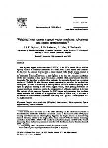
3.2. Surface representation and numerical derivatives The terms {gx , gy , gz} are numeric 1st derivatives of the unknown surface g (x, y, z). Their calculation depends on the analytical representation of the surface elements. p01 T{g0(x,y,z)} y
T{g0(x,y,z)}
n
z
f(x,y,z)
x
p11
w p00
(a)
n u
p10 y
f(x,y,z)
z x
(b)
Figure 1. Representation of surface elements in planar (a), and bi-linear (b) forms. Note that T{} stands for the transformation operator. As a first method, let us represent the search surface as composite of planar elements (Figure 1a), which are constituted by fitting a plane to 3 neighboring knot points, in the non-parametric implicit form g 0 ( x, y , z ) = Ax + By + Cz + D = 0
(3.21)
where A, B, C, and D are the parameters of the plane. The numeric 1st derivation according to the xaxis is
gx =
∂g 0 ( x, y, z ) g 0 ( x + Δx, y, z ) − g 0 ( x, y, z ) = lim Δx →0 ∂x Δx
(3.22)
where the numerator term of the equation is simply the distance between the plane and the off-plane point (x +Δx, y, z). Then using the point-to-plane distance formula, gx =
A( x + Δx) + By + Cz + D 2
2
Δx A + B + C
2
=
A
(3.23)
2
A + B2 + C 2
is obtained. Similarly gy and gz are calculated numerically:
gy =
B 2
2
A +B +C
, gz =
2
C
(3.24)
2
A + B2 + C 2
Actually, these numeric derivative values {gx , gy , gz} are x-y-z components of the local surface normal vector n at the exact correspondence location on the search surface:
[g
x
gy
gz
]
T
[
= n = nx
ny
] [A
nz =
B C]
T
A2 + B 2 + C 2
(3.25)
14
3.3. Numerical derivatives on the template surface
For the representation of the search surface as parametric bi-linear elements (Figure 1b), a bi-linear surface is fitted to 4 neighboring knot points pij : g 0 (u , w) = [x(u , w)
y (u , w) z (u , w)]
T
(3.26)
g 0 (u , w) = p00 (1 − u )(1 − w) + p01 (1 − u ) w + p10 u (1 − w) + p11uw
(3.27)
where u, w ∈ [0,1]2 and g0(u,w), pij ∈ ℜ3. The vector g0(u,w) is the position vector of any point on the bi-linear surface. Again the numeric derivative terms {gx , gy , gz} are calculated from components of the local surface normal vector n on the parametric bi-linear surface:
[g
x
gy
gz
]
T
= n=
∂g 0 (u , w) ∂g 0 (u , w) × ∂u ∂w
∂g 0 (u , w) ∂g 0 (u , w) × ∂u ∂w
(3.28)
where × stands for the vector cross product. With this approach a slightly better a posteriori sigma value could be obtained due to better surface modeling. Conceptually, derivative terms {gx , gy , gz} constitute a normal vector field with unit magnitude ||n||=1 on the search surface. This vector field slides over the template surface towards the final solution, minimizing the Least Squares objective function. The surface representation is carried out in two different forms optionally: a TIN form, which gives planar surface elements, and a grid mesh form, which gives bi-linear surface elements. Both of these are first degree C0 continuous surface representations. Surface topology is established simply by reading the standard range scanner output files in ASCII format and loading them in the scan-line order. For the pointclouds which have an irregular or unconventional sampling principle (or pattern), a more complex surface mesh generation algorithm can be utilized. In the case of multi-resolution data sets, in which point densities are significantly different on the template and search surfaces, higher degree C1 continuous composite surface representations, e.g. bicubic Hermit surface (Peters, 1974), should give better results, of course increasing the computational expenses.
3.3. Numerical derivatives on the template surface In the case of insufficient initial approximations, the numerical derivatives can also be calculated on the template surface f (x, y, z) instead of on the search surface g (x, y, z) in order to speed-up the convergence. This speed-up version apparently decreases the computational effort of the design matrix A as well, since the derivative terms {fx , fy , fz} are calculated only once in the first iteration, and the same values are used in the following iterations. The functional model of this version is given below. − e( x, y, z ) = f x d t x + f y d t y + f z d t z + ( f x a10 + f y a 20 + f z a30 ) d m + ( f x a11 + f y a 21 + f z a31 ) d ω + ( f x a12 + f y a 22 + f z a 32 ) d ϕ
(3.29)
+ ( f x a13 + f y a 23 + f z a 33 ) d κ − ( f ( x, y , z ) − g 0 ( x, y , z )) As opposed to the basic model, the number of the observation equations contributing to the design matrix A is here defined by the number of elements on the search surface g (x, y, z). In other words, the correspondence is searched on the template surface f (x, y, z) for each surface element of the search surface g (x, y, z). However, this is not a fully strict model. The derivative terms are approximated from the template surface. Comparisons against the strict model, given in Equation (3.10), show that the numerical differences of the solution vectors are not statistically significant.
15
3.4. Precision, reliability and error detection
Depending on the resolution or quality of the template or the search surfaces, either Equation (3.10) or Equation (3.29) can be selected for the functional model. Hence, the design matrix is established from the better surface, while the search surface is still floating and the template is fixed.
3.4. Precision, reliability and error detection The standard deviations of the estimated transformation parameters and the correlations between them may give useful information concerning the stability of the system and quality of the data content (Gruen, 1985a):
σˆ p = σˆ 0 q pp
,
q pp ∈ Q xx = ( A T PA + Pb ) −1
(3.30)
where Qxx is the cofactor matrix for the estimated parameters. The estimated standard deviations of the transformation parameters are optimistic, mainly due to the stochastic properties of the search surfaces that have not been considered as such in the estimation model, as is typically done in Least Squares matching (Gruen, 1985a). The omissions are expected to be minor and do not disturb the solution vector significantly. However, the a posteriori covariance matrix will be affected by the neglected uncertainty of the function values g (x, y, z). This deteriorates the realistic precision estimates. More details on this issue can be found in Gruen (1985a), Maas (2000), Gruen and Akca (2005) and Kraus et al. (2006). Detection of false correspondences with respect to the outliers and occlusions is a crucial part of every surface matching method. We use the following strategies in order to localize and eliminate the outliers and the occluded parts. A median type of filtering is applied prior to the matching. For each point, the distances between the central point and its k-neighborhood points are calculated. In our implementation, k is selected as 8. If most of those k-distance values are much greater than the average point density, the central point is likely to be an erroneous point on a poorly reflecting surface (e.g. window or glass) or a range artifact due to surface discontinuity (e.g. points on the object silhouette). The central point is discarded according to the number of distances, which are greater than a given distance threshold. In the course of iterations a simple weighting scheme adapted from Robust Estimation Methods is used: ⎧1 if | (v ) i |< Kσˆ 0 (P) ii = ⎨ ⎩0 else
(3.31)
In our experiments K is selected as >10, since it is aimed to suppress only the large outliers. It can be changed according to a desired confidence level. Because of the high redundancy of a typical data set, a certain amount of occlusions and/or smaller outliers do not have significant effect on the estimated parameters. As a comprehensive strategy, Baarda’s (1968) data-snooping method can be favorably used to localize the occluded or gross erroneous measurements. Finally, the correspondences coinciding to mesh boundaries are excluded from the estimation. The mesh boundaries represent the model borders, additionally the data holes inside the model. The data holes are possibly due to occlusions. Rejecting the correspondences on the mesh boundaries effectively eliminates the occlusions.
3.5. Convergence behavior In a standard Least Squares adjustment calculus, the function of the unknowns is unique, exactly known, and analytically continuous everywhere. Here the function g (x, y, z) is discretized by using a finite sampling rate, which leads to slow convergence, oscillations, even divergence in some cases with respect to the standard adjustment. The convergence behavior of the proposed method basically depends on the quality of the initial approximations and quality of the data content. For a good data configuration, it usually achieves the solution after 5 or 6 iterations (Figure 2), which is typical for the Least Squares matching.
16
3.6. Computational aspects dpi /ci ω 100
ω
(a)
tz κ
κ
tz
0 -100
(b)
tx φ
φ
ty 1
2
3
4
5
1
iterations
ty
tx 2
3
4
5
6
7
8
Figure 2. Typical examples for fast (a) and slow (b) convergence. Note that here the scale factor m is fixed to unity.
3.6. Computational aspects The computational effort increases with the number of points in the matching process. The main portion of the computational complexity is to search the corresponding elements of the template surface patch on the search surface, whereas the parameter estimation part is a small system, and is quickly solved using Cholesky decomposition followed by back-substitution. Searching the correspondence is guided by an efficient boxing structure (Chetverikov, 1991), which partitions the search space into cuboids. For a given surface element, the correspondence is searched only in the box containing this element and in the adjacent boxes. The details are given in Chapter 3.8.1.
3.7. The Generalized Gauss-Markoff versus Levenberg-Marquardt In Neugebauer (1997) and Szeliski and Lavallee (1996) two gradient descent type of algorithms are given. They calculate the Euclidean distances as evaluation function value by interpolation using point-to-projection and octree spline methods respectively. They adopt the Levenberg-Marquardt method, in which diagonal elements of the normal matrix N are augmented by a damping matrix D in order to prevent numerical problems: (N+λD)δ = n where λ>0 is the stabilization factor that varies during the iterations. The damping matrix D is often chosen as an identity matrix I or a diagonal matrix containing the diagonal elements of the normal matrix (diag(N)). The Generalized Gauss-Markoff model might be seen as identical to the Levenberg-Marquardt, as the weight matrix Pb has a damping effect on the normal matrix. But, it is a thorough statistical approach considering the a priori stochastic information (Equation 3.13), and a straightforward result of the Least Squares formulation (Equation 3.14). The Levenberg-Marquardt method is rather a numerical approach with no direct stochastical justification. Assume that two planes are the subject of the matching process. During the solution of a standard Least Squares adjustment, the normal matrix becomes singular, since there is not a unique solution geometrically. This numerical reflex issues a warning to the user. On the other hand, LevenbergMarquardt will give one of the solutions out of the infinite number. Geometrically ill-configured data sets are reasons for the near-singularity cases. When singularity or ill-conditioning occurs, one must carefully inspect the system and diagnose the data, instead of doing arbitrary numerical manipulations.
3.8. Acceleration strategies 3.8.1. Fast correspondence search with boxing structure Let points ai ={xi , yi , zi}∈S, i = 0,1,…, N-1, represent the object S∈ℜ3, and be kept in list L1 in spatially non-ordered form. The boxing data structure (Figure 3) consists of a rearranged point list L2 and an index matrix I = Iu,v,w whose elements are associated to individual boxes: u,v,w = 0,1,…, M-1.
17
3.8. Acceleration strategies
The items of L2 are coordinates of N points placed in the order of boxes. The index matrix I contains integers indicating the beginnings of the boxes in L2.
Initialization. Defining the box size. Step 1. Recall min, max{xi , yi , zi} of data volume. Step 2. Define number of boxes along x-y-z axes. For the sake of simplicity, they are given the same (M) here. Pass 1. Computing I. Step 1. Allocate an M x M x M size accumulator array B = Bu,v,w which is to contain the number of points in each box. Step 2. Scan L1 and fill B. For any point ai the box indices are as follows: ⎢ zi − zmin ⎥ ⎢ yi − ymin ⎥ ⎢ x − xmin ⎥ ui = ⎢ i ⎥ ⎥ , wi = ⎢ ⎥ , vi = ⎢ ⎣ DZ ⎦ ⎣ DY ⎦ ⎣ DX ⎦
(3.32)
where ⎣ ⎦ stands for the truncation operator, and DX , DY and DZ are dimensions of any box along the xy-z axes respectively. Step 3. Fill I using the following recursive formula: I 0 , 0 , 0 = 0. For all (u , v, w) ≠ (0,0,0)
I u ,v , w
⎧ I u ,v , w−1 + Bu ,v , w−1 ⎪ = ⎨ I u ,v −1, M −1 + Bu ,v −1, M −1 ⎪I ⎩ u −1, M −1, M −1 + Bu −1, M −1, M −1
if
w>0
else if
v>0
(3.33)
else
Pass 2. Filling L2. Step 1. For all u, v and w, set Bu,v,w = 0. Step 2. Scan L1 again. Use Equation (3.32), I and B to fill L2. In L2 , the first point of the (u,v,w)th box is indexed by I while the address of the subsequent points is controlled via B whose value is incremented each time a new point enters the box. Finally, release the memory area of B. The memory requirement is of order O(N) for L2 and O(M 3) for I. For the sake of clarity of the explanation, L2 is given as a point list containing the x-y-z coordinate values. If one wants to keep the L1 in the memory, then L2 should only contain the access indices to L1 or pointers, which directly point to the memory locations of the point coordinates.
Access procedure. Step 1. Using Equation (3.32), compute the indices ui , vi and wi of the box that contains point ai . Step 2. Use the boxing structure to retrieve the points bounded by the (u,v,w)-th box. In L2 , I indexes the first point, while the number of points in the box is given by the following formula: ⎧ I u , v , w +1 − I u ,v , w ⎪I ⎪ u , v +1,0 − I u , v , M −1 ⎨ ⎪ I u +1,0, 0 − I u , M −1, M −1 ⎪ N − I M −1, M −1, M −1 ⎩
if
w < M −1
else if
v < M −1
else if
u < M −1
(3.34)
else
The access procedure requires O(q) operations, where q is the average number of points in the box. One of the main advantages of the boxing structure is a faster and easier access mechanism than the tree search-based methods provide.
18
3.8. Acceleration strategies L2 Iu,v,w
z Any point ai in the box y
y o
z
x
x
x0 , y0 , z0 x1 , y1 , z1 … … Points of the (u,v,w)-th box
Figure 3. 3D Boxing. (left) Boxing binds all the data points, (right) the boxing data structure. The boxing structure, and in general all search structures, are designed for searching the nearest neighborhood in the static pointclouds. In the LS3D surface matching case, the search surface, which the boxing structure is established for, is transformed to a new state by the current set of transformation parameters. Nevertheless there is no need neither to re-establish the boxing structure nor to update the I and L2 in each iteration. Only positions of those four points (Figure 3) are updated in the course of iterations: o ={xmin , ymin , zmin}, x ={xmax , ymin , zmin}, y ={xmin , ymax , zmin}, z ={xmin , ymin , zmax}. They uniquely define the boxing structure under the similarity transformation. The access procedure is the same, except the following formula is used for the indices calculation: ⎢ oa ⋅ ox ⎥ ⎢ oa i ⋅ oy ⎥ ⎢ oa i ⋅ oz ⎥ ui = ⎢ i ⎥ , vi = ⎢ ⎥ , wi = ⎢ ⎥ ⎢⎣ ox D X ⎥⎦ ⎢⎣ oy DY ⎥⎦ ⎢⎣ oz D Z ⎥⎦
(3.35)
where · stands for vector dot product. If the transformation is a similarity rather than a rigid body, the DX , DY and DZ values must also be updated in the iterations. In our implementation, the correspondence is searched in the boxing structure during the first few iterations, and in the meantime its evolution is tracked across the iterations. Afterwards the searching process is carried out only in an adaptive local neighborhood according to the previous position and change of correspondence. In any step of the iteration, if the change of correspondence for a surface element exceeds a limit value, or oscillates, the search procedure for this element is returned to the boxing structure again.
3.8.2. Simultaneous multi-subpatch matching The basic estimation model can be implemented in a multi-patch mode, that is the simultaneous matching of two or more search surfaces g i(x, y, z), i =1,…, k to one template f (x, y, z). − e1 = A 1 x1 − l1 , P1
− e 2 = A 2 x 2 − l 2 , P2 M M − e k = A k x k − l k , Pk
(3.36)
Since the parameter vectors x1 ,…, xk do not have any joint components, the sub-systems of Equation (3.36) are orthogonal to each other. In the presence of auxiliary information, those sets of equations could be connected via functional constraints, e.g. as in the geometrically constrained multiphoto matching (Gruen, 1985a; Gruen and Baltsavias, 1988) or via appropriate formulation of multiple (>2) overlap conditions. An ordinary pointcloud includes enormously redundant information. A straightforward way to register such two pointclouds could be matching of the whole overlapping areas. This is computationally expensive. We propose multi-subpatch mode as a further extension to the basic model, which is capable of simultaneous matching of sub-surface patches, which are interactively selected in cooperative surface areas. They are joined to the system by the same 3D transformation parameters. This leads to the observation equations
19
3.9. Multiple surface matching
− e1 = A 1 x − l1 , P1
− e 2 = A 2 x − l 2 , P2 M M − e k = A k x − l k , Pk
(3.37)
with i =1,…, k subpatches. They can be combined as in Equation (3.11), since the common parameter vector x joints them to each other. The individual subpatches may not include sufficient information for the matching of whole surfaces, but together they provide a computationally effective solution, since they consist of only relevant information rather than using the full data set.
3.9. Multiple surface matching When more than two surfaces with multiple overlaps exist, the procedure is split into two steps: sequential pairwise registrations and a final global registration. The pairwise registrations establish the correspondences between the overlapping pairs of surfaces. The global registration distributes the residual errors evenly among all of the surfaces, and also considers the multiple overlap conditions and the closure condition, i.e. matching of the last surface to the first one. One of the surfaces is selected as the reference, which defines the datum of the common coordinate system. The pairwise LS3D matching processes are run on every possible overlapping surface pairs, starting from the datum one. Each matched surface is incrementally added to the union of the previously registered surfaces. If the search surface is already in the union, i.e. surface has multiple overlaps, the transformation is not applied. Each pairwise registration gives the 3D transformation parameters of the search surface and additionally the correspondences between the template and the search surfaces. These final correspondences are saved to separate files. Every individual correspondence gives a (fictitious) tie point. The numbers of tie points are thinned out by selecting of every n-th correspondence. Then, all these files are given as input to the block adjustment by independent models software BAM7, which is an in-house software based on a 7-parameter 3D similarity transformation. The block adjustment by independent models, which is a well-known orientation procedure in photogrammetry (Ackermann et al., 1973), was formerly proposed for the global registration of laser scanner pointclouds, but for the case of retro-reflective targets as tie points (Scaioni and Forlani, 2003). In the BAM7 software, (fictitious) points of the datum surface are treated as the control points. This leads the transformation parameters of the datum surfaces fixed in the procedure. The transformation parameters of all the other surfaces will be optimized regarding the global agreement of the whole data.
20
4.1. Formation of quasisurfaces
4 SIMULTANEOUS MATCHING OF SURFACE GEOMETRY AND INTENSITY When there is a lack of sufficient geometric information (homogeneity or isotropicity of curvatures), the procedure may fail, since there is not a unique solution geometrically, e.g. when matching two planes or spherical objects. An object surface may have some attribute information attached to it. Intensity, color and temperature are well known examples. Most of the laser scanners can supply intensity information in addition to the Cartesian coordinates for each point, or an additional camera may be used to collect texture. A solution is proposed that can simultaneously match intensity information and geometry under a combined estimation model. In this approach the intensity image of the pointcloud also contributes observation equations to the system, considering the intensities as supplementary information to the range image.
4.1. Formation of quasisurfaces Rather than adopting a feature-based or step-wise approach, this method sets up quasisurfaces from intensity information in addition to the actual surfaces. A hypothetical example of forming the quasisurfaces is given in Figure 4. The procedure starts with the calculation of surface normal vectors at each data point. The actual surface will include noise and surface spikes (Figure 4b), which lead to unrealistic calculations for the normal vectors. To cope with the problem, a moving average or median type filtering process could be employed. But still some noise would remain depending on the window size.
(a)
(b)
(d)
(c)
(e)
Figure 4. Forming the quasisurface. (a) Pointcloud with intensity information, (b) meshed surface of the pointcloud, (c) trend surface fitted to the pointcloud, (d) normal vectors attached onto the actual surface, (e) generated quasisurface in addition to the actual one.
21
4.2. Estimation model
An optimum solution is the Least Squares fitting of a global trend surface to the whole pointcloud (Figure 4c). It will suppress the noise component and preserve the global continuity of the normal vectors along the surface. The parametric bi-quadratic trend surface was chosen, which is sufficient to model the quadric type of surfaces, e.g. plane, sphere, ellipsoid, etc. For the template surface patch f (x, y, z) we obtain: 2
2
F (u , w) = ∑ ∑ bij u i w j
(4.1)
i =0 j =0
where u, w ∈ [0,1]2 , F(u,w) ∈ ℜ3 is the position vector of any point on the trend surface, and bij ∈ ℜ3 are the algebraic coefficients, which are estimated by Least Squares fitting. For each point, the normal vector nf is calculated on the trend surface F(u,w) and attached to the actual surface f (x, y, z) (Figure 4d): n f = n f (u , w) =
Fu × Fw Fu × Fw
(4.2)
where Fu and Fw are the tangent vectors along the u and w-axes, respectively. Finally, the quasisurface fc (x, y, z) is formed in such a way that each point of the actual surface f (x, y, z) is mapped along its normal vector nf up to a distance proportional to its intensity value cf (Figure 4e). f c ( x, y , z ) = f ( x, y , z ) + n f λ c f
(4.3)
where λ is an appropriate scalar factor for the conversion from the intensity range to the Cartesian space. Rather than the actual surface f (x, y, z), the trend surface F(u,w) can also be defined as the datum, which leads to f c ( x, y , z ) = F (u , w) + n f λc f
(4.4)
This isolates the geometric noise component from the quasisurface fc (x, y, z), but strongly smoothes the geometry. Equations (4.3) and (4.4) assume a fairly simplistic radiometric model (intensities are mapped perpendicular to the geometric surface). This model can be refined by considering an appropriate illumination model. The same procedure is performed for the search surface g (x, y, z) as well: g c ( x, y , z ) = g ( x , y , z ) + n g λ c g
(4.5)
4.2. Estimation model Equation (3.2) should also be valid for the quasisurfaces under the assumption that similar illumination conditions exist for both the template and search surfaces: f c ( x , y , z ) − e c ( x, y , z ) = g c ( x, y , z )
(4.6)
The random errors of the template and search quasisurfaces are assumed to be uncorrelated. The contrast and brightness differences or in the extreme case specular reflection will cause model errors, and deteriorate the reliability of the estimation. The radiometric variations between the template and search surface intensities should be reduced before matching by pre-processing or appropriate modeling in the estimation process by the use of extra parameters. For two images of an object acquired by an optical-passive sensor, e.g. a CCD camera, an intensity transfer function such as (cf = r0 + cg r1) could be suitable for the radiometric adaptation, where r0 (shift) and r1 (scale) are radiometric correction parameters. In the case of laser scanner derived 22
4.2. Estimation model
intensity images, the radiometric variations are strongly dependent on both the incident angle of the signal path with respect to the normal to the object surface and the object-to-sensor distance. Thus, for a plane type of object, the radiometric variations can be modeled in first approximation as in the following: f c ( x, y , z ) − e c ( x, y , z ) = g c ( x, y , z ) + r0 + ur1
(4.7)
where u is the abscissa of the search trend surface G(u,w), considering that the u-axis is the horizontal direction. In other words, the u-axis is the principal direction of change of the incident angles. Depending on the characteristics of the scan data, it can be replaced by the ordinate value w, or another type of parameterization. In general a second order bivariate polynomial (r0 + ur1 + wr2 + uwr3 + u2r4 + w2r5 + u2wr6 + uw2r7 + u2w2r8) or an appropriate subpart of it can be used. Although the radiometric parameters r0 and r1 are linear a priori, they are also expanded using the Taylor series. Equation (4.7) in linearized form gives: − e c ( x, y , z ) =
g c0 ( x, y , z ) g 0 ( x, y , z ) g 0 ( x, y , z ) dx+ c d y+ c d z + d r0 + u d r1 ∂x ∂y ∂z − ( f c ( x, y , z ) −
g c0 ( x,
y,
z ) − {r00
(4.8)
+ ur10 ; n g })
with notations g cx
∂g c0 ( x, y, z ) ∂g c0 ( x, y , z ) ∂g c0 ( x, y , z ) = , g cy = , g cz = ∂x ∂y ∂z
(4.9)
where the terms {gcx , gcy , gcz} stand for the numerical derivatives of the search quasisurface function. The first approximations of the radiometric parameters are r00 = r10 = 0. At the end of each iteration, the search quasisurface gc0(x, y, z) is transformed to a new state using the updated set of transformation parameters, and subsequently re-shaped by the current set of radiometric parameters r00 + ur10 along the normal vectors ng , which are calculated on the search trend surface G(u,w). The terms {dx , dy , dz} relate the Equations (3.4) and (4.8) to each other. The quasisurfaces are treated like actual surfaces in the estimation model. They contribute observation equations to the design matrix, joining the system by the same set of transformation parameters. After further expansion and with the assumptions E{ec}= 0 and E{ec ecT}= σ02Pc-1, Equation (4.8) becomes
− e c = A c x − l c , Pc
(4.10)
where ec , Ac , x, and Pc are the true error vector, the design matrix, the parameter vector, and the associated weight coefficient matrix for the quasisurface observations, respectively, and lc is the constant vector that contains the Euclidean distances between the template and corresponding search quasisurface elements. Here, the vector x is extended to include the radiometric parameters in addition to the transformation parameters. The hybrid system in Equations (3.11), (3.13) and (4.10) is of the combined adjustment type that allows simultaneous matching of geometry and intensity. The Least Squares solution of the system gives
xˆ = ( A T PA + Pb + A Tc Pc A c ) −1 ( A T Pl + P b l b + A Tc Pc l c )
(4.11)
In the experiments, weights for the quasisurface observations are selected as (Pc)ii < (P)ii , and the intensity measurements of the (laser) sensor are considered to be uncorrelated with the distance measurements (E{ec eT}= 0) for the sake of simplicity of the stochastic model.
23
4.2. Estimation model
24
5.1. Least squares 3D curve matching
5 FURTHER CONCEPTUAL EXTENSIONS 5.1. Least squares 3D curve matching Assume that two 3D curves of the same object are either directly measured by use of a contact measurement device, photogrammetric method, etc. or derived using any other technique. They can be matched in 3D space, since they represent the same object (Figure 5). The curves may have been measured or extracted in a point by point fashion, but can also be in different sampling patterns. Matching is established, if the sum of the squares of the Euclidean distances between the two curves is minimized by applying a 3D transformation to the search curve. The analytical representation of the curves is carried out in cubic spline form, but any other piecewise representation scheme can also be considered. In general, a parametric space curve is expressed, e.g. for the template curve, as: f (u ) = [x(u )
y (u ) z (u )]
T
(5.1)
where u ∈ [0,1] and f (u) ∈ ℜ3 is the position vector of any point on the curve. It has three components x(u), y(u), and z(u) which are considered as the Cartesian coordinates of the position vector (Rogers and Adams, 1976). y
z
x
Figure 5. Matching of free-form space curves. In the cubic spline representation 4
f (u ) = ∑ bi u i −1 = b1 + b2 u + b3 u 2 + b4 u 3
(5.2)
i =1
the coefficient vectors bi ∈ ℜ3 are determined by specifying the boundary conditions for the spline segments. The expanded form shows a 4th order 3rd degree analytical definition. A cubic degree ensures the second-order continuity (C2). This implies that the first (slope) and second (curvature) order derivatives are continuous across the joints of the composite curve. Similar expressions are also valid for the search curve: g (u ) = d 1 + d 2 u + d 3 u 2 + d 4 u 3
(5.3)
Using the parametric 3D space curve definition, the observation equations are formulated in the same manner as explained in Chapter 3: f (u ) − e(u ) = g (u )
(5.4)
25
5.1. Least squares 3D curve matching
Considering the same assumptions, which have been made in Chapter 3, with respect to the stochastic model, the geometric relationship between the template and search curves, and the Taylor expansion, the linearized functional model evolves as: f (u ) − e(u ) = g 0 (u ) +
∂g 0 (u ) du ∂u
(5.5)
f (u ) − e(u ) = g 0 (u ) +
∂g 0 (u ) ∂u ∂g 0 (u ) ∂u ∂g 0 (u ) ∂u dx+ dy+ dz ∂u ∂x ∂u ∂y ∂u ∂z
(5.6)
The relations between the Cartesian coordinate domains of the template and search curves are established via a 7-parameter 3D similarity transformation, where it is also possible to extend or reduce the parameter space of the 3D transformation upon necessity. The differentiation of the transformation equations results in: dx=
∂y ∂z ∂x d pi , d y = d pi , d z = d pi ∂pi ∂p i ∂p i
(5.7)
where pi ∈{tx , ty , tz , m, ω, φ, κ}is the i-th transformation parameter in Equation (3.3). The expression below ∂g 0 (u ) ⎡ ∂g 0 (u ) ∂u =⎢ ∂u ⎣ ∂u ∂x
∂g 0 (u ) ∂u ∂u ∂y
T
∂g 0 (u ) ∂u ⎤ ⎥ = gx ∂u ∂z ⎦
[
gy
gz
]
T
(5.8)
describes the numeric derivative terms. After further expansions, in the same manner as in Chapter 3, considering the parameters of the 3D transformation as fictitious observations, using an appropriate stochastic model, and with the assumptions E{e}= 0 and E{e eT}= σ02P-1, the system can be formulated as a Generalized Gauss-Markoff model: −e =A x−l , P
(5.9)
− eb = I x − l b , Pb
(5.10)
The Least Squares solution of the joint system Equations (5.9) and (5.10) gives the unbiased minimum variance estimation for the parameters: xˆ = ( A T PA + P b ) −1 ( A T Pl + P b l b )
solution vector
(5.11)
σˆ 02 = v T Pv + v bT P b v b r
variance factor
(5.12)
v = A xˆ − l
residual vector for curve observations
(5.13)
v b = I xˆ − l b
residual vector for parameter observations
(5.14)
The functional model is non-linear, and the solution is iterative. The iteration stops if each element of the alteration vector xˆ in Equation (5.11) falls below a certain limit. Let us assume that the first three derivatives do exist and are linearly independent for a point g (u) on a parametric curve (Figure 6). Then the first three derivatives g′(u), g′′(u), and g′′′(u) form a local affine coordinate system with origin g (u).
g ′′′
u
b
g (u )
n
u
g ′′ g′
g (u )
t
Figure 6. Local affine system (left) and Frenet frame (right) (adapted after Farin, 1997).
26
5.2. Matching of 3D curves with a 3D surface
From this local affine system, one can easily obtain a local Cartesian system with origin g (u) and axes t, n, b by the Gram-Schmidt process of orthonormalization (Farin, 1997):
t=
g′ g′
, b=
g ′ × g ′′ g ′ × g ′′
, n =b×t
(5.15)
The vectors t, n, b are called tangent, (main) normal, and bi-normal vectors, respectively. The frame t, n, b is called moving trihedron or Frenet frame. It varies its orientation as u traces out the curve (Farin, 1997). Considering this definition, the numeric 1st order derivative terms {gx , gy , gz} are the elements of the unit-length normal vector n at point g (u).
[g
x
gy
gz
]
T
=n
(5.16)
Using the proper degree and basis for curve representation, our method can handle multi-resolution and multi-sensor data sets, including multi-scale curves. It can be straightforwardly re-formulated in 2D for the matching of free-form image features.
5.2. Matching of 3D curves with a 3D surface The same formulation allows matching of one or more 3D curve(s) with a 3D surface simultaneously (Figure 7). The problem is finding the correspondence of a 1D geometric definition (curve) on a 2D geometric definition (surface), where both of them are parametrically represented in 3D space.
Figure 7. Matching of a 3D space curve with a 3D surface.
5.3. Matching of 3D sparse points with a 3D surface The LS3D method can match a 3D surface to a sparse set of 3D points provided that they have sufficiently good distribution. A set of ground control points (GCP) could be a good example for this case. This extension can be especially useful for the orientation or georeferencing of digital surface models.
5.4. Generalized multiple 3D surface and intensity matching Here, a method for the simultaneous co-registration and georeferencing of multiple 3D pointclouds and intensity information is proposed. It is a generalization of the 3D surface matching problem. The simultaneous co-registration provides for a strict solution to the problem, as opposed to sequential pairwise registration. The problem is formulated as the Least Squares matching of overlapping 3D surfaces. The parameters of 3D transformations of multiple surfaces are simultaneously estimated, using the Generalized Gauss-Markoff model, minimizing the sum of squares of the Euclidean distances among the surfaces. An observation equation is written for each surface-to-surface correspondence. Each overlapping surface pair contributes a group of observation equations to the design matrix.
27
5.4. Generalized multiple 3D surface and intensity matching
The parameters are introduced into the system as stochastic variables, as a second type of (fictitious) observations. This extension allows to control the estimated parameters. Intensity information is introduced into the system in the form of quasisurfaces as the third type of observations. Reference points, defining an external (object) coordinate system, which are imaged in additional intensity images, or can be located in the pointcloud, serve as the fourth type of observations. They transform the whole block of “models” to a pre-defined reference system. The total system is solved by applying the Least Squares technique, provided that sufficiently good initial values for the transformation parameters are given.
5.4.1. Least squares multiple 3D surface matching Assume a set of n surfaces of an object: g1(x, y, z) ,…, gn(x, y, z). The object is defined in a 3D Cartesian coordinate system, whereas the n surfaces are located in arbitrary local coordinate systems. The n surfaces are discrete 3D approximations of continuous function of object surface. They are digitized according to a sampling principle. There are m mutual spatial overlaps between the surfaces g i(x, y, z). Every overlap satisfies a pairwise matching: g i ( x, y, z ) − ei ( x, y, z ) = g j ( x, y, z ) , i, j = 1,..., n , i ≠ j
(5.17)
where e i(x, y, z) is a true error vector. It is assumed that i-th surface’s noise is independent of j-th one. Equations (5.17) are considered as nonlinear observation equations which model the observation vector g i(x, y, z) with functions g j(x, y, z). The Least Squares matching of the j-th surface to the i-th one is to be satisfied while the i-th surface is also subject to a 3D transformation (with respect to a predefined datum). This is the 3D case of the X-Y constraint version (i.e. grid sampling mode) of the multiphoto geometrically constrained matching (MPGC) (Gruen and Baltsavias, 1987) where both the template and the search image patches are transformed. Both surfaces are transformed to an object coordinate system while minimizing a goal function, which measures the sum of the squares of the Euclidean distances between them. The geometric relationships are established via 7-parameter similarity transformations. They can be replaced by another type if needed. In order to prevent the duplication, Equations (5.17) are written for every possible i-j pair where i8 or >10) to reduce type I errors confidently. Because of the high redundancy of a typical data set, a certain amount of occlusions and/or smaller outliers, i.e. type II errors, do not have significant effect on the estimated parameters. If it is a change detection or deformation study, the constant value K should be selected based on the a priori knowledge in order that the changed or deformed parts are appropriately excluded from the estimation. Since the estimation model is non-linear, the method needs initial approximations of the parameters. The initial approximations should be given or should be calculated prior to matching. To define a convergence radius value is extremely difficult. It depends on the geometric information of the object surface. It is our experience that the convergence is more sensitive to the initial values of the rotation angles than the translation elements. The capability of matching of surfaces of different quality and resolution is another positive aspect of the proposed method. This has two reasons. The first is certainly the rigorous mathematical formulation. The second is the selectivity of construction of the design matrix based on the choice of the better surface, either the template or the search surface, as explained in Chapter 3.3. The SRTM TerrainScape work, in cooperation with Swissphoto AG, proves this capability. Swissphoto AG has matched many DEMs all around the world with the SRTM C-SAR DEMs. The local DEMs are in any accuracy, point spacing and production techniques. According to their report, a complete failure case has not happened, except for some software debugging cases. The simultaneous multi-subpatch approach (Chapter 3.8.2) can be very useful for the change detection and deformation analysis studies in addition to computational acceleration. Change or deformation free parts (control patches) can be selected as cooperative multi-subpatches. Thus, inspection areas, which are probably deformed or changed, are confidently excluded from the registration. The forestry application exploits this feature. Experiments show that as long as the object surface has minimal information, e.g. in the case of very small structures on it, the basic algorithm, which uses only surface geometry, can find an acceptable solution. When the object surface is a plane or sphere, the surface geometry approach does not numerically fail as the sensor noise prevents the normal equation matrix from becoming singular. However, it finds a side minimum as the solution. In this case, the proposed method can find a reliable solution by introducing supplementary attribute information into the system. In the experiments, the laser scanner derived intensities were used as the supplementary information. The practical examples demonstrate the capability of the technique. Special attention should be paid to the radiometric variations between the surfaces. Additional radiometric correction parameters have been added to the mathematical model. This gives better results than the pre-processing option. The concept is not restricted to the registration of laser scanner pointclouds. It can find more application areas for cases where diverse types of attribute information are used.
7.3. Outlook Our experiences were very positive and the procedures worked very well. However, there is still need for further improvements and extensions. These are listed below. •
The iteration can start with a high order 3D transformation or a linear transformation with many terms, e.g. a 3D affine transformation. In the course of the iteration, non-determinable parameters are excluded by an appropriate determinability test. Thus, the parameter vector is adapted to the nature of the data in a self tuning and adaptive way.
•
As mentioned in Chapter 3.4, the search surface contains the stochastic properties unless it is an object surface which can be described analytically as a whole (without noise). This fact is neglected in the estimation model. As a more comprehensive model and in order to have
67
7.3. Outlook
realistic precision estimates, the estimation model can be replaced by an error-in-variables model. •
Due to the non-linear functional model, initial approximations of the parameters are needed. For full automation, a pre-alignment method can be integrated.
•
The current implementation uses two first degree surface representations (planar triangle mesh and bi-linear grid mesh). Higher order surface forms theoretically give better surface modeling (in sparse data cases), in consequence better results for the multi-resolution case, but with the cost of additional computational expense.
•
For the co-registration of multiple surfaces, a one step simultaneous solution as given in Chapter 5.4.1 should be realized.
•
The intensity matching approach uses a simple radiometric model, which maps the intensity values perpendicular to the geometric surface. This model should be improved by a strict model, which applies the mapping along the projection center to object surface considering the data acquisition geometry and radiometry (illumination conditions and sensor properties).
•
Implementations and testing of conceptual extensions are needed for
•
o
Least Squares 3D curve matching
o
matching of 3D curves with a 3D surface
o
matching of 3D sparse points with 3D surfaces
o
generalized multiple 3D surface and intensity matching
A combined co-registration and georeferencing approach might be very useful for many geodetic and photogrammetric applications. It performs the co-registration and the georeferencing tasks under one mathematical model simultaneously.
68
BIBLIOGRAPHY
BIBLIOGRAPHY Ackermann, F., Ebner, H., and Klein, H., 1973. Block triangulation with independent models. Photogrammetric Engineering and Remote Sensing 39 (9), 967-981. Ackermann, F., 1984. Digital image correlation: performance and potential application in photogrammetry. Photogrammetric Record 11 (64), 429-439. Akca, D., Remondino, F., Novàk, D., Hanusch, T., Schrotter, G., and Gruen, A., 2007. Performance evaluation of a coded structured light system for cultural heritage applictions. Videometrics IX, Proc. of SPIE-IS&T Electronic Imaging, San Jose (California), USA, January 29-30, SPIE vol. 6491, pp. 64910V-1-12. Akca, D., Gruen, A., Alkis, Z., Demir, N., Breuckmann, B., Erduyan, I., and Nadir, E., 2006. 3D modeling of the Weary Herakles statue with a coded structured light system. International Archives of the Photogrammetry, Remote Sensing and Spatial Information Sciences 36 (5), 14-19. Al-Manasir, K., and Fraser, C.S., 2006. Registration of terrestrial laser scanner data using imagery. The Photogrammetric Record 21 (115), 255-268. Arun, K.S., Huang, T.S., and Blostein, S.D., 1987. Least-squares fitting of two 3D point sets. IEEE Transactions on Pattern Analysis and Machine Intelligence 9 (5), 698-700. Baarda, W., 1968. A testing procedure for use in geodetic networks. Netherlands Geodetic Commission, Delft, Vol. 2, No. 5, 97 p. Baltsavias, E., Gruen, A., Küchler, M., Thee, P., Waser, L.T., and Zhang, L., 2006. Tree height measurements and tree growth estimation in a mire environment using digital surface models. In Proceedings of Workshop on 3D Remote Sensing in Forestry, 14 – 15 February, Vienna, Austria, 9 p. Available at ftp://igpho.ethz.ch/ ub/manos/papers/vienna06_manos.pdf (accessed 23 October 2006). Beinat, A., and Crosilla, F., 2001. Generalized Procrustes analysis for size and shape 3D object reconstructions. Optical 3-D Measurement Techniques V, Vienna, October 1-4, pp. 345-353. Benjemaa, R., and Schmitt, F., 1997. Fast global registration of 3D sampled surfaces using a multi-zbuffer technique. IEEE International Conference on 3D Digital Imaging and Modeling, Ottawa, pp. 113-120. Bentley, J.L., 1975. Multidimensional binary search trees used for associative searching. Communication of the ACM 18 (9), 509-517. Bergevin, R., Soucy, M., Gagnon, H., and Laurendeau, D., 1996. Towards a general multi-view registration technique. IEEE Transactions on Pattern Analysis and Machine Intelligence 18 (5), 540-547. Besl, P.J., and McKay, N.D., 1992. A method for registration of 3D shapes. IEEE Transactions on Pattern Analysis and Machine Intelligence 14 (2), 239-256. Blais, G., and Levine, M.D., 1995. Registering multiview range data to create 3D computer objects. IEEE Transactions on Pattern Analysis and Machine Intelligence 17 (8), 820-824. Blais, F., Taylor, J., Cournoyer, L., Picard, M., Borgeat, L., Dicaire, L.G., Rioux, M., Beraldin, J.-A., Godin, G., Lahanier, C., and Aitken, G., 2005. Ultra-high resolution imaging at 50 µm using a portable XYZ-RGB color laser scanner. Int. Workshop on Recording, Modeling and Visualization of Cultural Heritage, Ascona, May 22-27, (on CD-ROM). Breuckmann, B., 2003. State of the art of topometric 3D-metrology. Optical 3-D Measurement Techniques VI, Zurich, Switzerland, Sept. 22-25, Vol. II, pp. 152-158.
69
BIBLIOGRAPHY
Brinkhoff, T., 2004. Spatial access methods for organizing laserscanner data. International Archives of Photogrammetry, Remote Sensing and Spatial Information Sciences 35 (B4), 98-102. Brodie, N., Doole, J., and Watson, P., 2000. Stealing history: The illicit trade in cultural material. The McDonald Institute of Archaeological Research, Cambridge, UK, pp. 31-32. Brodie, N., 2003. Stolen history: looting and illicit trade. Museum International 55 (3-4), 10-22. Campbell, R.J., and Flynn, P.J., 2001. A survey of free-form object representation and recognition techniques. Computer Vision and Image Understanding 81 (2), 166-210. Chen, Y., and Medioni, G., 1992. Object modelling by registration of multiple range images. Image and Vision Computing 10 (3), 145-155. Chetverikov, D., 1991. Fast neighborhood search in planar point sets. Pattern Recognition Letters 12 (7), 409-412. Chetverikov, D., Stepanov, D., and Krsek, P., 2005. Robust Euclidean alignment of 3D point sets: the trimmed iterative closest point algorithm. Image and Vision Computing 23 (3), 299-309. Cohen, F.S., and Wang, J.Y., 1994. Part I: Modeling image curves using invariant 3-D object curve models – A path to 3-D recognition and shape estimation from image contours. IEEE Transactions on Pattern Analysis and Machine Intelligence 16 (1), 1-12. Cunnington, S.J., and Stoddart, A.J., 1999. N-view point set registration: a comparison. British Machine Vision Conference, Nottingham, pp. 234-244. Dalley, G., and Flynn, P., 2002. Pair-wise range image registration: a case study in outlier classification. Computer Vision and Image Understanding 87 (1-3), 104-115. Danielsson, P.-E, 1980. Euclidean distance mapping. Computer Graphics and Image Processing 14 (3), 227-248. D’Apuzzo, N., 2002. Measurement and modeling of human faces from multi images. International Archives of Photogrammetry, Remote Sensing and Spatial Information Sciences 34 (5), 241-246. Dorai, C., Weng, J., and Jain, A.K., 1997. Optimal registration of object views using range data. IEEE Transactions on Pattern Analysis and Machine Intelligence 19 (10), 1131-1138. Ebner, H., and Mueller, F., 1986. Processing of Digital Three Line Imagery using a generalized model for combined point determination. International Archives of Photogrammetry and Remote Sensing 26 (3/1), 212-222. Ebner, H., Fritsch, D., Gillessen, W., and Heipke, C., 1987. Integration von bildzuordnung und objektrekonstruktion innerhalb der digitalen photogrammetrie. BuL 55 (5), 194-203. Ebner, H., and Strunz, G., 1988. Combined point determination using Digital Terrain Models as control information. International Archives of Photogrammetry and Remote Sensing 27 (B11/3), 578-587. Ebner, H., Strunz, G., and Colomina, I., 1991. Block triangulation with aerial and space imagery using DTM as control information. ACSM-ASPRS Annual Convention, Technical Papers, Baltimore, March 25-29, vol.5, pp. 76-85. Ebner, H., and Ohlhof, T., 1994. Utilization of Ground Control Points for image orientation without point identification in image space. International Archives of Photogrammetry and Remote Sensing 30 (3/1), 206-211. Eggert, D.W., Lorusso, A., and Fisher, R.B., 1997. Estimating 3-D rigid body transformations: a comparison of four major algorithms. Machine Vision and Applications 9 (5-6), 272-290. Eggert, D.W., Fitzgibbon, A.W., and Fisher, R.B., 1998. Simultaneous registration of multiple range views for use in reverse engineering of CAD models. Computer Vision and Image Understanding 69 (3), 253-272.
70
BIBLIOGRAPHY
Farin, G., 1997. Curves and surfaces for computer-aided geometric design. Fourth edition, Academic Press, USA, pp. 173-174. Faugeras, O.D., and Hebert, M., 1986. The representation, recognition, and locating of 3-D objects. The International Journal of Robotics Research 5 (3), 27-52. Feldmar, J., and Ayache, N., 1996. Rigid, affine and locally affine registration of free-from surfaces. International Journal of Computer Vision 18 (2), 99-119. Fitzgibbon, A.W., 2001. Robust registration of 2D and 3D point sets. British Machine Vision Conference, Manchester, September 10-13, pp. 411-420. Forkert, G., Kerschner, M., Prinz, R., and Rottensteiner, F., 1995. Reconstruction of free-formed spatial curves from digital images. International Archives of Photogrammetry and Remote Sensing 30 (5/W1), 163-168. Gizzarelli, C., 2006. ‘Weary Herakles’: Looters vs. Archaeologists, http://www.bellaonline.com/articles/art28239.asp (accessed 6 April 2006). Godin, G., Laurendeau, D., and Bergevin, R., 2001. A method for the registration of attributed range images. IEEE International Conference on 3D Digital Imaging and Modeling, Quebec, May 28 – June 1, pp. 179-186. Golub, G.H., and Van Loan, C.F., 1980. An analysis of the total least squares problem. SIAM Journal on Numerical Analysis 17 (6), 883-893. Greaves, T., 2005. Laser scanning shaves weeks from failure analysis of parking garage collapse. Spar ViewTM 3 (14), http://www.sparllc.com/archiveviewer.php?vol=03&num=14&file=vol03no14-01 (accessed August 2005). Gruen, A., 1984. Adaptive least squares correlation – concept and first results. Intermediate Research Project Report to Heleva Associates, Inc., Ohio State University, Columbus, Ohio, March, pp. 113. Gruen, A., 1985a. Adaptive least squares correlation: a powerful image matching technique. South African Journal of Photogrammetry, Remote Sensing and Cartography 14 (3), 175-187. Gruen, A., 1985b. Adaptive kleinste Quadrate Korrelation und geometrische Zusatzinformationen. Vermessung, Photogrammetrie, Kulturtechnik, 9/85, 309-312. Gruen, A., 1985c. Data processing methods for amateur photographs. Photogrammetric Record 11 (65), 567-579. Gruen, A., and Baltsavias, E.P., 1987. High precision image matching for digital terrain model generation. Photogrammetria 42 (3), 97-112. Gruen, A., and Baltsavias, E.P., 1988. Geometrically Constrained Multiphoto Matching. Photogrammetric Engineering and Remote Sensing 54 (5), 633-641. Gruen, A., and Stallmann, D., 1991. High accuracy edge matching with an extension of the MPGC matching algorithm. International Conference on Industrial Vision Metrology, Winnipeg, July 1112, SPIE vol. 1526, pp. 42-55. Gruen, A., and Agouris, P., 1994. Linear feature extraction by least squares template matching constrained by internal shape forces. International Archives of Photogrammetry and Remote Sensing 30 (3/1), 316-323. Gruen, A., and Li, H., 1996. Linear feature extraction with LSB-Snakes from multiple images. International Archives of Photogrammetry and Remote Sensing 31 (3B), 266-272. Gruen, A., 1996. Least squares matching: a fundamental measurement algorithm. In: K. Atkinson (ed.), Close Range Photogrammetry and Machine Vision, Whittles, pp. 217-255. Gruen, A., and Akca, D., 2005. Least squares 3D surface and curve matching. ISPRS Journal of Photogrammetry and Remote Sensing 59 (3), 151-174.
71
BIBLIOGRAPHY
Greenspan, M., and Godin, G., 2001. A nearest neighbor method for efficient ICP. IEEE International Conference on 3D Digital Imaging and Modeling, Quebec, pp. 161-168. Greenspan, M., and Yurick, M., 2003. Approximate K-D tree search for efficient ICP. IEEE International Conference on 3D Digital Imaging and Modeling, Banff, pp.442-448. Guehring, J., 2001. Reliable 3D surface acquisition, registration and validation using statistical error models. IEEE International Conference on 3D Digital Imaging and Modeling, Quebec, May 28June 1, pp. 224-231. Gueziec, A., and Ayache, N., 1994. Smoothing and matching of 3-D space curves. International Journal of Computer Vision 12 (1), 79-104. Helava, U.V., 1988. Object-space least-squares correlation. Photogrammetric Engineering and Remote Sensing 54 (6), 711-714. Horn, B.K.P., 1987. Closed-form solution of absolute orientation using unit quaternions. Journal of the Optical Society of America A-4 (4), 629-642. Horn, B.K.P., Hilden, H.M., and Negahdaripour, S., 1988. Closed-form solution of absolute orientation using orthonormal matrices. Journal of the Optical Society of America A-5 (7), 11281135. Inan, J., 1981. Perge kazısı 1980 çalışmaları. III KST, DSİ Basım ve Foto Film İşletme Müdürlüğü Matbaası, Ankara, sayfa 43-48 (in Turkish). Inan, J., 1992. Heraklesstatue vom Typus des “Herakles Fernese” aus Perge. Festschrift für Max Wegner Zum 90. Geburtstag, Bonn, pp. 223-232. Jackins, C.L., and Tanimoto, S.L., 1980. Oct-trees and their use in representing three-dimensional objects. Computer Graphics and Image Processing 14 (3), 249-270. Jaw, J.J., 2000. Control surface in aerial triangulation. International Archives of Photogrammetry and Remote Sensing 33 (B3), 444-451. Johnson, A.E., and Kang, S.B., 1999. Registration and integration of textured 3D data. Image and Vision Computing 17 (2), 135-147. Jokinen, O., and Haggren, H., 1998. Statistical analysis of two 3-D registration and modeling strategies. ISPRS Journal of Photogrammetry and Remote Sensing 53 (6), 320-341. Jokinen, O., 1998. Area-based matching for simultaneous registration of multiple 3-D profile maps. Computer Vision and Image Understanding 71 (3), 431-447. Jost, T., and Huegli, H., 2003. A multi-resolution ICP with heuristic closest point search for fast and robust 3D registration of range images. IEEE International Conference on 3D Digital Imaging and Modeling, Banff, pp. 427-433. Karras, G.E., and Petsa, E., 1993. DEM matching and detection of deformation in close-range Photogrammetry without control. Photogrammetric Engineering and Remote Sensing 59 (9), 14191424. Kishon, E., Hastie, T., and Wolfson, H., 1991. 3-D curve matching using splines. Journal of Robotic Systems 8 (6), 723-743. Kraus, K., Ressl, C., and Roncat, A., 2006. Least squares matching for airborne laser scanner data. 5th International Symposium Turkish-German Joint Geodetic Days, Berlin, March 29-31, (only on CDROM). Krishnan, S., Lee, P.Y., Moore J.B., and Venkatasubramanian, S., 2005. Global registration of multiple 3D point sets via optimization-on-a-manifold. Eurographics Symposium on Geometry Processing, Vienna, July 4-6, pp. 187-197. Langis, C., Greenspan, M., and Godin, G., 2001. The parallel iterative closest point algorithm. IEEE International Conference on 3D Digital Imaging and Modeling, Quebec, pp. 195-204.
72
BIBLIOGRAPHY
Lavallee, S., Szeliski, R., and Brunie, L., 1991. Matching 3-D smooth surfaces with their 2-D projections using 3-D distance maps. Geometric Methods in Computer Vision, San Diego, July 2526, SPIE vol.1570, pp. 322-336. Lu, F., and Milios, E., 1997. Globally consistent range scan alignment for environment mapping. Autonomous Robots 4 (4), 333-349. Maas, H.G., 1994. A high-speed solid state camera system for the acquisition of flow tomography sequences for 3D least squares matching. International Archives of Photogrammetry and Remote Sensing 30 (5), 241-249. Maas, H.G., and Gruen, A., 1995. Digital photogrammetric techniques for high resolution three dimensional flow velocity measurements. Optical Engineering 34 (7), 1970-1976. Maas, H.G., 2000. Least-Squares Matching with airborne laserscanning data in a TIN structure. International Archives of Photogrammetry and Remote Sensing 33 (3A), 548-555. Maas, H.G., 2001. On the use of pulse reflectance data for laserscanner strip adjustment. International Archives of Photogrammetry, Remote Sensing and Spatial Information Sciences 34 (Part 3/W4), 53-56. Masuda, T., and Yokoya, N., 1995. A robust method for registration and segmentation of multiple range images. Computer Vision and Image Understanding 61 (3), 295-307. Mitchell, H.L., and Chadwick, R.G., 1999. Digital Photogrammetric concepts applied to surface deformation studies. Geomatica 53 (4), 405-414. Museum Rietberg, 2006. Exhibition Brochure. Neugebauer, P.J., 1997. Reconstruction of real-world objects via simultaneous registration and robust combination of multiple range images. International Journal of Shape Modeling 3 (1-2), 71-90. Norris, G., 2005. Jeppesen puts synthetic vision system on display. Flight International, 25-31 October, 9-10. Okatani, I.S., and Deguchi, K., 2002. A method for fine registration of multiple view range images considering the measurement error properties. Computer Vision and Image Understanding 87 (1-3), 66-77. Pajdla, T., and Van Gool, L., 1995. Matching of 3-D curves using semi-differential invariants. Proc. of IEEE International Conference on Computer Vision, Cambridge (MA), June 20-23, pp. 390-395. Park, S.-Y., and Subbarao, M., 2003. A fast point-to-tangent plane technique for multi-view registration. IEEE International Conference on 3D Digital Imaging and Modeling, Banff, pp. 276283. Parsi, B.K., Jones, J.L., and Rosenfeld, A., 1991. Registration of multiple overlapping range images: Scenes without distinctive features. IEEE Transactions on Pattern Analysis and Machine Intelligence 13 (9), 857-871. Pertl, A., 1984. Digital image correlation with the analytical plotter Planicomp C-100. International Archives of Photogrammetry and Remote Sensing 25 (3B), 874-882. Peters, G.J., 1974. Interactive computer graphics application of the parametric bi-cubic surface to engineering design problems. In: R. Barnhill and R. Riesenfeld (Eds.), Computer Aided Geometric Design, Academic Press, pp. 259-302. Pilgrim, L., 1996. Robust estimation applied to surface matching. ISPRS Journal of Photogrammetry and Remote Sensing 51 (5), 243-257. Planitz, B.M., Maeder, A.J., and Williams, J.A., 2005. The correspondence framework for 3D surface matching algorithms. Computer Vision and Image Understanding 97 (3), 347-383.
73
BIBLIOGRAPHY
Poli, D., Zhang, L., and Gruen, A., 2004. SPOT-5/HRS stereo images orientation and automated DSM generation. International Archives of Photogrammetry, Remote Sensing and Spatial Information Sciences 35 (B1), 421- 432 (and on DVD). Postolov, Y., Krupnik, A., and McIntosh, K., 1999. Registration of airborne laser data to surfaces generated by Photogrammetric means. International Archives of Photogrammetry and Remote Sensing 32 (3/W14), 95-99. Potmesil, M., 1983. Generating models of solid objects by matching 3D surface segments. International Joint Conference on Artificial Intelligence, Karlsruhe, August 8-12, pp. 1089-1093. Pottmann, H., Leopoldseder, S., and Hofer, M., 2004. Registration without ICP. Computer Vision and Image Understanding 95 (1), 54-71. Pulli, K., Duchamp, T., Hoppe, H., McDonald, J., Shapiro, L., and Stuetzle, W., 1997. Robust meshes from multiple range maps. IEEE International Conference on 3D Digital Imaging and Modeling, Ottawa, pp. 205-211. Pulli, K., 1999. Multiview registration for large data sets. IEEE International Conference on 3D Digital Imaging and Modeling, Ottawa, October 4-8, pp. 160-168. Rogers, D.F., and Adams, J.A., 1976. Mathematical elements for computer graphics. McGraw-Hill Book Company, London, pp. 116-155. Rose, M., and Acar, O., 1995. Turkey’s war on the illicit antiquities trade. Archaeology 48 (2), 45-56. Rosenholm, D., and Torlegard, K., 1988. Three-dimensional absolute orientation of stereo models using Digital Elevation Models. Photogrammetric Engineering and Remote Sensing 54 (10), 13851389. Roth, G., 1999. Registering two overlapping range images. IEEE International Conference on 3D Digital Imaging and Modeling, Ottawa, October 4-8, pp. 191-200. Rusinkiewicz, S., and Levoy, M., 2001. Efficient variants of the ICP algorithm. IEEE International Conference on 3D Digital Imaging and Modeling, Quebec, May 28 – June 1, pp. 145-152. Sauerbier, M., Kunz, M., Fluehler, M., and Remondino, F., 2004. Photogrammetric reconstruction of adobe architecture at Tucume, Peru. International Archives of Photogrammetry, Remote Sensing and Spatial Information Sciences 36 (5/W1), (only on CD-Rom). Scaioni, M., and Forlani, G., 2003. Independent model triangulation of terrestrial laser scanner data. International Archives of the Photogrammetry, Remote Sensing and Spatial Information Sciences 34 (5/W12), 308-313. Schaffrin, B., and Felus, Y.A., 2003. On total least-squares adjustment with constraints. In Proceedings of IUGG General Assembly, Sapporo, Japan, June 30-July 11. Schenk, T., Krupnik, A., and Postolov, Y., 2000. Comparative study of surface matching algorithms. International Archives of Photogrammetry and Remote Sensing 33 (B4), 518-524. Schoenemann, P.H., and Carroll, R.M., 1970. Fitting one matrix to another under choice of a central dilation and a rigid motion. Psychometrika 35 (2), 245-255. Schwartz, J.T., and Sharir, M., 1987. Identification of partially obscured objects in two and three dimensions by matching noisy characteristic curves. The International Journal of Robotics Research 6 (2), 29-44. Sharp, G.C., Lee, S.W., and Wehe, D.K., 2004. Multiview registration of 3D scenes by minimizing error between coordinate frames. IEEE Transactions on Pattern Analysis and Machine Intelligence 26 (8), 1037-1050. Sternberg, H., Kersten, Th., Jahn, I., and Kinzel, R., 2004. Terrestrial 3D laser scanning – data acquisition and object modeling for industrial as-built documentation and ar-chitectural
74
BIBLIOGRAPHY
applications. International Archives of the Photogrammetry, Remote Sensing and Spatial Information Sciences 35 (B7), 942-947. Stoddart, A.J., and Hilton, A., 1996. Registration of multiple point sets. IEEE International Conference on Pattern Recognition, Vienna, pp. B40- 44. Szeliski, R., and Lavallee, S., 1996. Matching 3-D anatomical surfaces with non-rigid deformations using octree-splines. International Journal of Computer Vision 18 (2), 171-186. Turk, G., and Levoy, M., 1994. Zippered polygon meshes from range images. Proc. of ACM SIGGRAPH’94, Orlando (Florida), July 24-29, pp. 311-318. Xu, Z., and Li, Z., 2000. Least median of squares matching for automated detection of surface deformations. International Archives of Photogrammetry and Remote Sensing 33 (B3), 1000-1007. Vanden Wyngaerd, J., and Van Gool, L., 2003. Combining texture and shape for automatic crude patch registration. IEEE International Conference on 3D Digital Imaging and Modeling, Banff, Canada, October 6-10, pp. 179-186. Wang, J.Y., and Cohen, F.S., 1994. Part II: 3-D object recognition and shape estimation from image contours using B-splines, shape invariant matching, and Neural Networks. IEEE Transactions on Pattern Analysis and Machine Intelligence 16 (1), 13-23. Wang, J., and Shan, J., 2005. Lidar data management with 3-D Hilbert space-filling curve. ASPRS Annual Meeting, Baltimore, March 7-11, (only on CD-ROM). Waser, L.T., Küchler, M., Baltsavias, E., Feldmeyer-Christe, E., Eisenbeiss, H., Ginzler, C., Three, P., and Zhang, L., 2007. Assessing changes of forest area and shrub encroachment in a mire ecosystem using digital surface models and CIR-aerial images. Remote Sensing of Environment (accepted for publication). Weik, S., 1997. Registration of 3-D partial surface models using luminance and depth information. IEEE International Conference on Recent Advances in 3D Digital Imaging and Modeling, Ottawa, Canada, May 12-15, pp. 93-100. Wendt, A., and Heipke, C., 2006. Simultaneous orientation of brightness, range and intensity images. International Archives of Photogrammetry, Remote Sensing and Spatial Information Sciences 36 (5), 315-322. Williams, J.A., Bennamoun, M., and Latham, S., 1999. Multiple view 3D registration: A review and a new technique. IEEE International Conference on Systems, Man, and Cybernetics, Tokyo, October 12-15, pp. 497-502. Williams, J., and Bennamoun, M., 2001. Simultaneous registration of multiple corresponding point sets. Computer Vision and Image Understanding 81 (1), 117-142. Wrobel, B., 1987. Facets Stereo Vision (FAST Vision) – a new approach to computer stereo vision and to digital photogrammetry. Proceedings of ISPRS intercommission conference on fast processing of photogrammetric data, Interlaken, Switzerland, June 2-4, pp. 231-258. Yoshida, K., and Saito, H., 2002. Registration of range images using texture of high-resolution color images. IAPR Workshop on Machine Vision Applications (MVA’02), Nara, December 11-13, pp. 150-153. Zalmanson, G.H., and Schenk, T., 2001. Indirect orientation of pushbroom sensors with 3-D free-form curves. Joint Workshop of ISPRS on High Resolution Mapping from Space, Hannover, September 19-21 (on CD-ROM). Zhang, Z., 1994. Iterative point matching for registration of free-form curves and surfaces. International Journal of Computer Vision 13 (2), 119-152. Zhang, L., and Gruen, A., 2004. Automatic DSM Generation from Linear Array Imagery Data. International Archives of Photogrammetry, Remote Sensing and Spatial Information Sciences 35 (B3), 128-133.
75
BIBLIOGRAPHY
Zhang, L., Kocaman, S., Akca, D., Kornus, W., and Baltsavias, E., 2006. Test and performance evaluation of DMC images and new methods for their processing. ISPRS Commission I Symposium, Paris, July 3-6, (only on CD-ROM).
76
ACKNOWLEDGEMENTS I would like to present my gratitude to Prof. Dr. Armin Gruen for giving me the opportunity of a Ph.D. study under his supervision, for encouraging me to work on the Least Squares matching topic and for providing me an excellent research environment and conditions. His direct support, invaluable advices, solid knowledge and excellent problem-analysis skills have directed me in reaching my research goals, confidentially. I also appreciate his patience and persistence not only in scientific aspects but also in personal manners. His outstanding scientist and exceptional supervisor sides will have a strong influence on my future life. My gratitude is extended to my co-referent Prof. Dr. Orhan Altan of the Istanbul Technical University, Turkey. My early work under his supervision constitutes the foundation of the presented work here. I thank him by heart for his help and great support both academically and personally. I was very fortunate to have had the opportunity to work with him. Many thanks go to Dr. Emmanuel Baltsavias for his invaluable suggestions and very fruitful discussions. His suggestions have broadened the application areas of the LS3D surface matching method. I would like to thank Dr. Nicola D’Appuzo for providing the “human face” data set, Mr. Martin Vögele (Leica Geosystems AG, Zurich, Switzerland) and Mr. Peter Glueck (Leica Geosystems HDS Inc., Rijswijk, The Netherlands) for providing the “industrial plant” data set, Mr. Hans Woerner (Breuckmann GmbH, Meersburg, Germany) for providing “newspaper” data set, Mr. Martin Sauerbier (Institute of Geodesy and Photogrammetry, ETH Zurich, Switzerland) for providing the “Tucume” data set, Mr. Martin Reinkoester (Zoller+Fröhlich GmbH Elektrotechnik, Wangen, Germany) for providing the “bas-relief” and “chapel” data sets, Dr. Thorsten Schulz (Institute of Geodesy and Photogrammetry, ETH Zurich, Switzerland) for providing the “ball” data set, Dr. Thomas Abmayr (Zoller+Fröhlich GmbH Elektrotechnik, Wangen, Germany) for providing the “wall painting” data set, Dr. Emmanuel Baltsavias (Institute of Geodesy and Photogrammetry, ETH Zurich, Switzerland) for providing the data sets given in Chapter 6.3.6 and 6.3.7, and Dr. Li Zhang (Institute for Photogrammetry and Remote Sensing, Chinese Academy of Surveying and Mapping, Beijing, P.R. China) for providing the reference DSM given in Chapter 6.3.8. My special thanks go to Mr. Marcel Andriesse (formerly with Swissphoto AG, Zurich, Switzerland) for initiating the SRTM TerrainScape™ project. His feedbacks have significantly improved the operational capabilities of the LS3D software. I thank Thomas Hanusch for translating the English abstract to German. Help, care and friendliness of Beat Ruedin, our system administrator, Mrs. Gertrud Rothenberger, Mrs. Liliane Steinbrückner and Mrs. Susanne Sebestyen, our institute secretaries, is also greatly appreciated. Many thanks go to my actual and former colleagues at the Group of Photogrammetry and Remote Sensing for their useful suggestions on my work, their help, and their friendliness. Finally, I am grateful to the below “people cloud” for giving me (in any kind of form) help, support and self-sacrifice. Their value is known by my hearth, individually for each: “…………………………………...” Devrim Akca
77
CURRICULUM VITAE M.Sc. Mehmet Devrim Akca Institute of Geodesy and Photogrammetry ETH Zurich HIL D52.3 Wolfgang-Pauli-Str. 15 8093 Zurich Personal Date of birth: Nationality: Formation 2003 – 2007: 2000 – 2002: 1997 – 2000:
1993 – 1997: 1989 – 1993:
May 27, 1975 Turkish Ph.D. degree, Institute of Geodesy and Photogrammetry, ETH Zurich, Switzerland, Ph.D. Thesis: Least squares 3D surface matching. Ph.D. student (not finished), Department of Geodesy and Photogrammetry, Istanbul Technical University, Turkey. M.Sc. degree, Department of Geodesy and Photogrammetry, Karadeniz Technical University, Trabzon, Turkey, M.Sc. Thesis: Modeling environmental data using GIS: Case study of Trabzon - Degirmendere Valley. B.Sc. degree, Department of Geodesy and Photogrammetry, Karadeniz Technical University, Trabzon, Turkey. Cadastre technician degree, Anatolian Land Registry and Cadastre High School, Ankara, Turkey.
Employment 2003 – 2007: Research assistant, Chair of Photogrammetry and Remote Sensing, Institute of Geodesy and Photogrammetry, ETH Zurich, Switzerland. 2002 – 2003: Academic guest, Chair of Photogrammetry and Remote Sensing, Institute of Geodesy and Photogrammetry , ETH Zurich, Switzerland. 2001 – 2002: Research assistant, Division of Photogrammetry, Department of Geodesy and Photogrammetry, Istanbul Technical University, Turkey. 2000 – 2001: Research and teaching assistant, Department of Geodesy and Photogrammetry, Ondokuz Mayis University, Samsun, Turkey. 1997 – 2000: Surveying engineer, Cadastre Office, Macka (Trabzon), Turkey. 1993 – 1994: Cadastre technician, Cadastre Office, Yenice (Zonguldak), Turkey. Awards and Honors • Listing in Marquis Who’s Who in Science and Engineering, 9th edition, 2006-2007. • The ISPRS Prize for Best Papers by Young Authors, 20th ISPRS Congress, 2004. • Doctoral fellowship, Scientific and Technical Council of Turkey (TUBITAK), 2001-2002. • Honorary degree in B.Sc. graduation (First rank of the department), Karadeniz Technical University, Turkey, 1997. Publications 17 publications at conferences and journals and 6 technical reports since 2003. A complete list of publications is available at http://www.photogrammetry.ethz.ch/general/persons/devrim_publ.html Languages Native language: Turkish Foreign languages: English, German
78