The feasible set of standard form linear program has at least .... Simplex method:
An example ..... Matlab code: bintprog for solve binary integer linear.
Lecture 2: Branch-and-Bound Method (3 units) Outline I
Linear program
I
Simplex method
I
Dual of linear programming
I
Branch-and-bound method
I
Software for integer programming
1 / 32
Linear Program I
Recall that the standard form of LP: min c T x s.t. Ax = b x ≥0 where c ∈ Rn , A is an m × n matrix with full row rank, b ∈ Rm .
I
A polyhedron is a set of the form {x ∈ Rn | Bx ≥ d} for some matrix B.
I
Let P ∈ Rn be a given polyhedron. A vector x ∈ P is an extreme point of P if there does not exist y , z ∈ P, and λ ∈ (0, 1) such that x = λy + (1 − λz).
2 / 32
Basic Solutions and Extreme Points I
Let S = {x ∈ Rn | Ax = b, x ≥ 0}, the feasible set of LP. Since A is full row rank, if the feaisble set is not empty, then we must m ≤ n. WLOG, we assume that m < n.
I
Let A = (B, N), where B is an m × m matrix with full rank, i.e., det(B) 6= 0. Then, B is called a basis. µ ¶ xB Let x = .We have BxB + NxN = b. Setting xN = 0 , xN µ −1 ¶ B b −1 we have xB = B b. x = is called a basic 0 solution. xB is called basic variables, xN is called nonbasic variables.
I
I
If theµbasic solution is also feasible, this is, B −1 b ≥ 0, then ¶ −1 B b x= is called a basic feasible solution. 0 3 / 32
Basic Solutions and Extreme Points I
xˆ ∈ S is an extreme point of S if and only if xˆ is a basic feasible solution.
I
Two extreme points are adjacent if they differ in only one basic variable.
I
(Basic Theorem of LP) Consider the linear program min{c T x | Ax = b, x ≥ 0}. If S has at least one extreme point and there exists an optimal solution, then there exists an optimal solution that is an extreme point.
I
Proof (representation of polyhedron)
I
The feasible set of standard form linear program has at least one extreme point.
I
Therefore, we claim that the optimal value of a linear program is either −∞, or is attained an extreme point (basic feasible solution) of the feasible set. 4 / 32
A naive algorithm for linear programming
I I
I I
Let min{c T x | Ax = b, x ≥ 0} be a bounded LP ¶ µ m Enumerate all bases B ∈ {1, . . . , , n}, = O(nm ) many n µ −1 ¶ B b Compute associated basic solution x = 0 Return the one which has largest objective function value among the feasible basic solutions
I
Running time is O(nm · m3 )!!!
I
Are there more efficient algorithms?
5 / 32
Simplex method I
I
I
Simplex method was invented by George Dantzig (1914–2005) (father of linear programming) µ −1 ¶ B b Suppose we have a basic feasible solution xˆ = , 0 A = (B, N). Let xµ∈ S be µ ¶ any feasible ¶solution of the LP. Let xB cB x= ,c= . Then BxB + NxN = b and so xN cN xB = B −1 b − B −1 NxN cT x
= cBT xB + cNT xN = cBT B −1 b − cBT B −1 NxN + cNT xN = c T xˆT + (cNT − cBT B −1 N)xN
I
Let rN = cNT − cBT B −1 N (called reduced cost). If rN ≥ 0, then c T x ≥ c T xˆT and the current extreme point xˆ is optimal 6 / 32
Simplex method I
Otherwise, there must exist an ri < 0, we can let current nonbasic variable xi become a basic variable xi > 0 (entering variable).
I
Suitably choosing basic variable to become a nonbasic variable (leaving variable), we can get a new basic feasible solution whose objective value is less than that of the current basic feasible solution xˆ.
I
Geometrically, the above method (simplex method) moves from one extreme point to one of its adjacent extreme point.
I
Since there are only a finite number of extreme points, the method terminates finitely at an optimal solution or detects that the problem is infeasible or it is unbounded.
7 / 32
Geometry of Simplex Method
Figure: Simplex method 8 / 32
Simplex method I
Step 0: Compute initial µ an ¶ basis B and the basic feasible B −1 b solution: x = . 0
I
Step 1: If rN = cNT − cBT B −1 N ≥ 0, stop, x is an optimal solution, otherwise go to Step 2.
I
Step 2: Choose j satisfying cjT − cBT B −1 aj < 0, if ¯aj = B −1 aj ≤ 0, stop, the LP is infinite; otherwise, go to Step 3.
I
Step 3. Compute the stepsize: b¯i b¯r | ¯aij > 0} = ≥ 0. ¯aij ¯arj µ ¶ −B −1 aj Let x := x + λdj , where dj = . Go to Step 1. ej λ = min{
9 / 32
Simplex Tableau
xB B cBT
xN N cNT
rhs xB b =⇒ I 0 0
xN B −1 N cNT − cBT B −1 N
rhs B −1 b −cBT B −1 b
10 / 32
Simplex method: An example I
Consider the following LP: min − 7x1 − 2x2 s.t. − x1 + 2x2 + x3 = 4, 5x1 + x2 + x4 = 20, 2x1 + 2x2 − x5 = 7, x ≥ 0.
I
The initial tableau is x1 −1 5 2 −7
x2 2 1 2 −2
x3 1 0 0 0
x4 0 1 0 0
x5 0 0 −1 0
rhs 4 20 7 0 11 / 32
I
Choose the initial basis: B = (a1 , a3 , a4 ), basic variable: xB = (x1 , x3 , x4 )T . The simplex tableau is: x1 0 0 1 0
I
x2 3 −4 1 5
x3 1 0 0 0
x4 0 1 0 0
x5 − 12 2 12 − 12 − 72
rhs 7 12 2 12 3 12 24 12
The basic feasible solution is: xB = (x1 , x3 , x4 )T = (3 12 , 7 21 , 2 21 )T . Since − 72 < 0, choose x5 as the entering variable, λ =
2 12 2 12
= 1, so x4 is leaving variable,
the new basic variable is xB = (x1 , x3 , x5 ). The new tableau is x1 0 0 1 0
x2
11 5 − 85 1 5 − 53
x3 1 0 0 0
x4 1 5 2 5 1 5 7 5
x5 0 1 0 0
rhs 8 1 4 28 12 / 32
I
Choose x2 as the entering variable, compute 8 4 λ = min{ 11/5 , 1/5 } = 40 11 . x3 is the leaving variable, the new tableau is: x1 0 0 1 0
x2 1 0 0 0
x3
5 11 8 11 1 − 11 3 11
x4 1 11 6 11 2 11 16 11
x5 0 1 0 0
rhs 40 11 75 11 36 11 2 30 11
3 16 Since rN = ( 11 , 11 ) ≥ 0, the current basic feasible solution 36 40 T x = ( 11 , 11 , 0, 0, 75 11 ) is the optimal solution with optimal 2 value: −30 11 .
13 / 32
Dual theory: motivation I
Consider the following minimization problem with a single equality constraint: (P)
min f (x) s.t. h(x) = 0, x ∈ X,
where h(x) = 0 is a hard constraint and x ∈ X is a “easy” constraint. I
How could we solve this problem? The idea is to relax the hard constraint h(x) = 0 and solve an easier problem.
I
This can be done by incorporating the constraint into the objective function. A price is associated if the constraint is violated. 14 / 32
I
Given a Lagrangian multiplier λ (price), the Lagrangian dual function defined by d(λ) = min L(x, λ) := f (x) + λh(x) x∈X
gives a lower bound for (P): d(λ) ≤ f (x),
I
The best lower bound is found by solving (D)
I
∀ feasible solution of(P).
max d(λ). λ
(D) is called the Lagrangian dual problem of (P).
15 / 32
Dual of Linear Program I
Consider the standard LP: (LP)
min c T x s.t. Ax = b, x ≥ 0,
I
Associate multipliers λ ∈ Rm to Ax = b, the dual function is d(λ) = min{c T x + λT (b − Ax)} = b T λ + min(c − AT λ)T x x≥0 x≥0 ½ T T b λ, if A λ ≤ c = −∞, otherwise
I
So, the dual problem is (LD)
max b T λ s.t. AT λ ≤ c.
16 / 32
Inequality Constraints I
Consider the standard LP: min c T x
(LP)
s.t. Ax ≥ b, x ≥ 0, I
Adding slack variables s ≥ 0, we get µ ¶ x (A, −I ) = b. s
I
This leads to dual constraints T
µ
(A, −I ) λ ≤ I
c 0
¶ .
Hence, the dual of LP is: (LD)
max b T λ s.t. AT λ ≤ c λ ≥ 0.
17 / 32
Primal and Dual Forms We can dualize general LPs as follows: ¯ ¯ ¯ min c T x ¯ max b T y ¯ ¯ ¯ ¯ ≥ ≥ ≤ ≥ ¯ (LP) ¯ ⇔(LD) ¯¯ T ≤ ≤ ≥ ≤ 0 s.t. Ax b, x 0 s.t. A y c, y ¯ ¯ ¯ ¯ = free = free Primal (Minimize) Constraints
Variables
Dual (Maximize) ≥ bi ≤ bi = bi ≥0 ≤0 free
⇔ ⇔ ⇔ ⇔ ⇔ ⇔
≥0 ≤0 free ≤ cj ≥ cj = cj
Variables
Constraints
18 / 32
Branch-and-Bound Method
I
Branch-and-bound strategy: I
I
I
Solve the linear relaxation of the problem. If the solution is integer, then we are done. Otherwise create two new subproblems by branching on a fractional variable. A node (subproblem) is not active when any of the following occurs: (1)The node is being branched on; (2) The solution is integral; (3) The subproblem is infeasible; (4) You can fathom the subproblem by a bounding argument. Choose an active node and branch on a fractional variable. Repeat until there are no active subproblems.
19 / 32
Branch-and-bound search tree:
20 / 32
I
Example. Consider the following 0-1 knapsack problem: max 8x1 + 11x2 + 6x3 + 4x4 s.t. 5x1 + 7x2 + 4x3 + 3x4 ≤ 14 x ∈ {0, 1}4 .
I
The linear relaxation solution is x = (1, 1, 0.5, 0) with a value of 22. The solution is not integral.
I
Choose x3 to branch. The next two subproblems will have x3 = 0 and x3 = 1 respectively.
21 / 32
I
The search tree is:
I
The linear relaxation solutions to the two subproblems are I I
I
x3 = 0: x = (1, 1, 0, 0.667), objective value=21.65; x3 = 1: x = (1, 0.714, 1, 0), objective value=21.85.
At this point we know that the optimal value is no more than 21.85 (we actually know it is less than or equal to 21. but we still do not have any feasible integer solution. So, we will take a subproblem and branch on one of its variables. 22 / 32
I
Choose the node with x3 = 1 and branch on x2 . The branch tree is:
I
The linear relaxation solutions are I I
x3 = 1, x2 = 0: x = (1, 1, 1, 1), objective value=18; x3 = 1: x2 = 1: x = (0.6, 1, 1, 0), objective value=21.8. 23 / 32
I
Choose node with x3 = 1, x2 = 0 and branch on x1 . The search tree is
I
The linear relaxation solutions are I I
I
x3 = 1, x2 = 0, x1 = 0: x = (0, 1, 1, 1), objective value=21; x3 = 1: x2 = 1: x1 = 1: infeasible.
The optimal solution is x = (0, 1, 1, 1). 24 / 32
Solving 0-1 Knapsack by B&B I
0-1 Knapsack Problem (01KP)
I
max{c T x | aT x ≤ b, x ∈ {0, 1}n }.
To solve the LP relaxation of (01KP), you need only be greedy! Assume that the variables have been ordered such that c1 /a1 ≥ c2 /a2 ≥ · · · ≥ cn /an .
(1)
Let s be the maximum index k such that k X
aj ≤ b.
(2)
j=1
25 / 32
I
Theorem (Dantzig (1957)): The optimal solution to the continuous relaxation of (01KP) is wj = 1, j = 1, . . . , s, wj = 0, j = s + 2, . . . , N, s X ws+1 = (b − aj )/as+1 . j=1
I
If cj , j = 1, . . . , N, are positive integers, then an upper bound of the optimal value of (LKP) is given by UB =
s X j=1
cj + b(b −
s X
aj )cs+1 /as+1 c,
(3)
j=1
26 / 32
How to Branch? I
We want to divide the current problem into two or more subproblems that are easier than the original. A commonly used branching method: xi ≤ bxi∗ c, xi ≥ dxi∗ e,
I
I
I
I
where xi∗ is a fractional variable. Which variable to branch? A commonly used branching rule: Branch the most fractional variable. We would like to choose the branching that minimizes the sum of the solution times of all the created subproblems. How do we know how long it will take to solve each subproblem? Answer: We don’t. Idea: Try to predict the difficulty of a subproblem. A good branching rule: The value of the linear programming relaxation changes a lot! 27 / 32
Which Node to Select?
I
An important choice in branch and bound is the strategy for selecting the next subproblem to be processed.
I
Goals: (1) Minimizing overall solution time. (2) Finding a good feasible solution quickly.
I
Some commonly used search strategies: I I I I
Best First Depth-First Hybrid Strategies Best Estimate
28 / 32
The Best First Approach
I
I
One way to minimize overall solution time is to try to minimize the size of the search tree. We can achieve this by choosing the subproblem with the best bound (lowest lower bound if we are minimizing). Drawbacks of Best First I
I
I
Doesn’t necessarily find feasible solutions quickly since feasible solutions are “more likely” to be found deep in the tree Node setup costs are high. The linear program being solved may change quite a bit from one node evaluation to the next Memory usage is high. It can require a lot of memory to store the candidate list, since the tree can grow “broad”
29 / 32
The Depth First Approach I
The depth first approach is to always choose the deepest node to process next. Just dive until you prune, then back up and go the other way
I
This avoids most of the problems with best first: The number of candidate nodes is minimized (saving memory). The node set-up costs are minimized
I
LPs change very little from one iteration to the next. Feasible solutions are usually found quickly
I
Drawback: If the initial lower bound is not very good, then we may end up processing lots of non-critical nodes.
I
Hybrid Strategies: Go depth-first until you find a feasible solution, then do best-first search
30 / 32
The nodes expanded in depth-first branch-and-bound search:
31 / 32
Software for integer programming
I
Matlab code: bintprog for solve binary integer linear programming problems.
I
Commercial optimization software CPLEX and Gurobi for solving mixed integer linear and quadratic programming problems. Two simple ways of calling CPLEX MIP solver:
I
I
I
I
Optimization Programming Language (OPL) in CPLEX Optimization Studio. CPLEX Matlab interface.
Examples using Matlab and CPLEX
32 / 32