lectures on the combinatorial structure of the moduli spaces of ...

LECTURES ON THE COMBINATORIAL STRUCTURE OF THE MODULI SPACES OF RIEMANN SURFACES AND FEYNMAN DIAGRAM EXPANSION OF MATRIX INTEGRALS MOTOHICO MULASE

Contents 1. Riemann Surfaces and Elliptic Functions 1.1. Basic Definitions 1.2. Elementary Examples 1.3. Weierstrass Elliptic Functions 1.4. Elliptic Functions and Elliptic Curves 1.5. Degeneration of the Weierstrass Elliptic Function 1.6. The Elliptic Modular Function 1.7. Compactification of the Moduli of Elliptic Curves 2. Matrix Integrals and Feynman Diagram Expansion 2.1. Asymptotic Expansion of Analytic Functions 2.2. Feynman Diagram Expansion 2.3. Preparation from Graph Theory 2.4. Asymptotic Analysis of 1 × 1 Matrix Integrals 2.5. The Logarithm and the Connectivity of Graphs 2.6. Ribbon Graphs and Oriented Surfaces 2.7. Hermitian Matrix Integrals 2.8. M¨ obius Graphs and Non-Orientable Surfaces 2.9. Symmetric Matrix Integrals References

1 1 3 10 13 16 20 27 31 31 36 38 43 48 50 53 58 65 68

1. Riemann Surfaces and Elliptic Functions 1.1. Basic Definitions. Let us begin with defining Riemann surfaces and their moduli spaces. Definition 1.1 (Riemann surfaces). A Riemann surface is a paracompact HausS dorff topological space C with an open covering C = λ Uλ such that for each open set Uλ there is an open domain Vλ of the complex plane C and a homeomorphism φλ : Vλ −→ Uλ

(1.1)

that satisfies that if Uλ ∩ Uµ 6= ∅, then the gluing map φ−1 µ ◦ φλ (1.2)

φ−1 µ

φλ

−1 Vλ ⊃ φ−1 λ (Uλ ∩ Uµ ) −−−−→ Uλ ∩ Uµ −−−−→ φµ (Uλ ∩ Uµ ) ⊂ Vµ

Date: March 14, 2009. 1

2

MOTOHICO MULASE

is a biholomorphic function. C U1 U2 φ2

φ1 φ−1 φ1 2 °

V1

V2

Figure 1.1. Gluing two coordinate charts. Remark. (1) A topological space X is paracompact if S for every open covering S X = λ Uλ , there is a locally finite open cover X = i Vi such that Vi ⊂ Uλ for some λ. Locally finite means that for every x ∈ X, there are only finitely many Vi ’s that contain x. X is said to be Hausdorff if for every pair of distinct points x, y of X, there are open neighborhoods Wx 3 x and Wy 3 y such that Wx ∩ Wy = ∅. (2) A continuous map f : V −→ C from an open subset V of C into the complex plane is said to be holomorphic if it admits a convergent Taylor series expansion at each point of V ⊂ C. If a holomorphic function f : V −→ V 0 is one-to-one and onto, and its inverse is also holomorphic, then we call it biholomorphic. (3) Each open set Vλ gives a local chart of the Riemann surface C. We often identify Vλ and Uλ by the homeomorphism φλ , and say “Uλ and Uµ are glued by a biholomorphic function.” The collection {φλ : Vλ −→ Uλ } is called a local coordinate system. (4) A Riemann surface is a complex manifold of complex dimension 1. We call the Riemann surface structure on a topological surface a complex structure. The definition of complex manifolds of an arbitrary dimension can be given in a similar manner. For more details, see [19]. Definition 1.2 (Holomorphic functions on a Riemann surface). A continuous function f : C −→ C defined on a Riemann surface C is said to be a holomorphic function if the composition f ◦ φλ φλ

f

Vλ −−−−→ Uλ ⊂ C −−−−→ C is holomorphic for every index λ. Definition 1.3 (Holomorphic maps between Riemann surfaces). A continuous map h : C −→ C 0 from a Riemann surface C into another Riemann surface C 0 is a holomorphic map if the composition map (φ0µ )−1 ◦ h ◦ φλ φλ

h

φ0µ

Vλ −−−−→ Uλ ⊂ C −−−−→ C 0 ⊃ Uµ0 −−−−→ Vµ0 is a holomorphic function for every local chart Vλ of C and Vµ0 of C 0 .

MODULI OF RIEMANN SURFACES

3

Definition 1.4 (Isomorphism of Riemann surfaces). If there is a bijective holomorphic map h : C −→ C 0 whose inverse is also holomorphic, then the Riemann surfaces C and C 0 are said to be isomorphic. We use the notation C ∼ = C 0 when they are isomorphic. Since the gluing function (1.2) is biholomorphic, it is in particular an orientation preserving homeomorphism. Thus each Riemann surface C carries the structure of an oriented topological manifold of real dimension 2. We call it the underlying topological manifold structure of C. The orientation comes from the the natural orientation of the complex plane. All local charts are glued in an orientation preserving manner by holomorphic functions. A compact Riemann surface is a Riemann surface that is compact as a topological space without boundary. In these lectures we deal mostly with compact Riemann surfaces. The classification of compact topological surfaces is completely understood. The simplest example is a 2-sphere S 2 . All other oriented compact topological surfaces are obtained by attaching handles to an oriented S 2 . First, let us cut out two small disks from the sphere. We give an orientation to the boundary circle that is compatible with the orientation of the sphere. Then glue an oriented cylinder S 1 × I (here I is a finite open interval of the real line R) to the sphere, matching the orientation of the boundary circles. The surface thus obtained is a compact oriented surface of genus 1. Repeating this procedure g times, we obtain a compact oriented surface of genus g. The genus is the number of attached handles. Since the sphere has Euler characteristic 2 and a cylinder has Euler characteristic 0, the surface of genus g has Euler characteristic 2 − 2g. A set of marked points is an ordered set of distinct points (p1 , p2 , · · · , pn) of a Riemann surface. Two Riemann surfaces with marked points C, (p1 , · · · , pn ) and C 0 , (p01 , · · · , p0n ) are isomorphic if there is a biholomorphic map h : C −→ C 0 such that h(pj ) = p0j for every j. Definition 1.5 (Moduli space of Riemann surfaces). The moduli space Mg,n is the set of isomorphism classes of Riemann surfaces of genus g with n marked points. The goal of these lectures is to give an orbifold structure to Mg,n × Rn+ and to determine its Euler characteristic for every genus and n > 0. 1.2. Elementary Examples. Let us work out a few elementary examples. The simplest Riemann surface is the complex plane C itself with the standard complex structure. The unit disk D1 = {z ∈ C |z| < 1} of the complex plane is another example. We note that although these Riemann surfaces are homeomorphic to one another, they are not isomorphic as Riemann surfaces. Indeed, if there was a biholomorphic map f : C −→ D1 , then f would be a bounded (since |f | < 1) holomorphic function defined entirely on C. From Cauchy’s integral formula, one concludes that f is constant. The simplest nontrivial example of a compact Riemann surface is the Riemann sphere P1 . Let U1 and U2 be two copies of the complex plane, with coordinates z and w, respectively. Let us glue U1 and U2 with the identification w = 1/z for z 6= 0. The union P1 = U1 ∪ U2 is a compact Riemann surface homeomorphic to the 2-dimensional sphere S 2 . The above constructions give all possible complex structures on the 2-plane R2 and the 2-sphere S 2 , which follows from the following:

4

MOTOHICO MULASE

Theorem 1.6 (Riemann Mapping Theorem). Let X be a Riemann surface with trivial fundamental group: π1 (X) = 1. Then X is isomorphic to either one of the following: (1) the entire complex plane C with the standard complex structure; (2) the unit disk {z ∈ C |z| < 1} with the standard complex structure induced from the complex plane C; or (3) the Riemann sphere P1 . Remark. The original proof of the Riemann mapping theorem is due to Riemann, Koebe, Carath´eodory, and Poincar´e. Since the technique we need to prove this theorem has nothing to do with the topics we deal with in these lectures, we refer to [41], volume II, for the proof. We note that P1 is a Riemann surface of genus 0. Thus the Riemann mapping theorem implies that M0 consists of just one point. A powerful technique to construct a new Riemann surface from a known one is the quotient construction via a group action on the old Riemann surface. Let us examine the quotient construction now. Let X be a Riemann surface. An analytic automorphism of X is a biholomorphic map f : X −→ X. The set of all analytic automorphisms of X forms a group through the natural composition of maps. We denote by Aut(X) the group of analytic automorphisms of X. Let G be a group. When there is a group homomorphism φ : G −→ Aut(X), we say the group G acts on X. For an element g ∈ G and a point x ∈ X, it is conventional to write g(x) = (φ(g))(x), and identify g as a biholomorphic map of X into itself. Definition 1.7 (Fixed point free and properly discontinuous action). Let G be a group that acts on a Riemann surface X. A point x ∈ X is said to be a fixed point of g ∈ G if g(x) = x. The group action of G on X is said to be fixed point free if no element of G other than the identity has a fixed point. The group action is said to be properly discontinuous if for every compact subsets Y1 and Y2 of X, the cardinality of the set {g ∈ G g(Y1 ) ∩ Y2 6= ∅} is finite. Remark. A finite group action on a Riemann surface is always properly discontinuous. When a group G acts on a Riemann surface X, we denote by X/G the quotient space, which is the set of orbits of the G-action on X. Theorem 1.8 (Quotient construction of a Riemann surface). If a group G acts on a Riemann surface X properly discontinuously and the action is fixed point free, then the quotient space X/G has the structure of a Riemann surface. Proof. Let us denote by π : X −→ X/G the natural projection. Take a point x b ∈ X/G, and choose a S point x ∈ π −1 (b x) of X. Since X is covered by local coordinate systems X = µ Uµ , there is a coordinate chart Uµ that contains x. Note that we can cover each Uµ by much smaller open sets without changing the Riemann surface structure of X. Thus without loss of generality, we can assume


5

that Uµ is a disk of radius centered around x, where is chosen to be a small positive number. Since the closure U µ is a compact set, there are only finitely many elements g in G such that g(U µ ) intersects with U µ . Now consider taking the limit → 0. If there is a group element g 6= 1 such that g(U µ ) ∩ U µ 6= ∅ as becomes smaller and smaller, then x ∈ U µ is a fixed point of g. Since the G action on X is fixed point free, we conclude that for a small enough , g(U µ ) ∩ U µ = ∅ for every g 6= 1. Therefore, π −1 (π(Uµ )) is the disjoint union of g(Uµ ) for all distinct g ∈ G. Moreover, (1.3)

π : Uµ −→ π(Uµ )

gives a bijection between Uµ and π(Uµ ). Introduce the quotient topology to X/G by defining π(Uµ ) as an open neighborhood of x b ∈ X/G. With respect to the quotient topology, the projection π is continuous and locally a homeomorphism. Thus we can introduce a holomorphic coordinate system to X/G by (1.3). The gluing function of π(Uµ ) and π(Uν ) is the same as the gluing function of Uµ and g(Uν ) for some g ∈ G such that Uµ ∩ g(Uν ) 6= ∅, which is a biholomorphic function because X is a Riemann surface. This completes the proof. Remark. (1) The above theorem generalizes to the case of a manifold. If a group G acts on a manifold X properly discontinuously and fixed point free, then X/G is also a manifold. (2) If the group action is fixed point free but not properly discontinuous, then what happens? An important example of such a case is a free Lie group action on a manifold. A whole new theory of fiber bundles starts here. (3) If the group action is properly discontinuous but not fixed point free, then what happens? The quotient space is no longer a manifold. Thurston coined the name orbifold for such an object. We will study orbifolds in later sections. Definition 1.9 (Fundamental domain). Let G act on a Riemann surface X properly discontinuously and fixed point free. A region Ω of X is said to be a fundamental domain of the G-action if the disjoint union of g(Ω), g ∈ G, covers the entire X: a X= g(Ω). g∈G

The simplest Riemann surface is C. What can we obtain by considering a group action on the complex plane? First we have to determine the automorphism group of C. If f : C −→ C is a biholomorphic map, then f cannot have an essential singularity at infinity. (Otherwise, f is not bijective.) Hence f is a polynomial in the coordinate z. By the fundamental theorem of algebra, the only polynomial that gives a bijective map is a polynomial of degree one. Therefore, Aut(C) is the group of affine transformations C 3 z 7−→ az + b ∈ C, where a 6= 0. Exercise 1.1. Determine all subgroups of Aut(C) that act on C properly discontinuously and fixed point free.

6

MOTOHICO MULASE

Let us now turn to the construction of compact Riemann surfaces of genus 1. Choose an element τ ∈ C such that Im(τ ) > 0, and define a free abelian subgroup of C by Λτ = Z · τ ⊕ Z · 1 ⊂ C.

(1.4)

This is a lattice of rank 2. An elliptic curve of modulus τ is the quotient abelian group (1.5) Eτ = C Λτ . It is obvious that the natural Λτ -action on C through addition is properly discontinuous and fixed point free. Thus Eτ is a Riemann surface. Figure 1.2 shows a fundamental domain Ω of the Λτ -action on C. It is a parallelogram whose four vertices are 0, 1, 1 + τ , and τ . It includes two sides, say the interval [0, 1) and [0, τ ), but the other two parallel sides are not in Ω.

τ

1+τ Ω

0

1

Figure 1.2. A fundamental domain of the Λτ -action on the complex plane. Topologically Eτ is homeomorphic to a torus S 1 × S 1 . Thus an elliptic curve is a compact Riemann surface of genus 1. Conversely, one can show that if a Riemann surface is topologically homeomorphic to a torus, then it is isomorphic to an elliptic curve. Exercise 1.2. Show that every Riemann surface of genus 1 is an elliptic curve. (Hint: Let Y be a Riemann surface and X its universal covering. Show that X has a natural complex structure such that the projection map π : X −→ Y is locally biholomorphic.) An elliptic curve Eτ = C Λτ is also an abelian group. The group action by addition Eτ × Eτ 3 (x, y) 7−→ x + y ∈ Eτ is a holomorphic map. Namely, for every point y ∈ Eτ , the map x 7−→ x + y is a holomorphic automorphism of Eτ . Being a group, an elliptic curve has a privileged point, the origin 0 ∈ Eτ . When are two elliptic curves Eτ and Eµ isomorphic? Note that since Im(τ ) > 0, τ and 1 form a R-linear basis of R2 = C. Let ω1 a b τ = , ω2 c d 1 where

a c

b ∈ SL(2, Z). d


7

Then the same lattice Λτ is generated by (ω1 , ω2 ): Λτ = Z · ω1 ⊕ Z · ω2 . Therefore, (1.6)

Eτ = C (Z · ω1 ⊕ Z · ω2 ).

To make (1.6) into the form of (1.5), we divide everything by ω2 . Since the division by ω2 is a holomorphic automorphism of C, we have Eτ = C (Z · ω1 ⊕ Z · ω2 ) ∼ = Eµ , where (1.7)

τ 7−→ µ =

ω1 aτ + b = . ω2 cτ + d

The above transformation is called a linear fractional transformation, which is an of a modular transformation. Note that we do not allow the matrix example a b to have determinant −1. This is because when the matrix has determinant c d −1, we can simply interchange ω1 and ω2 so that the net action is obtained by an element of SL(2, Z). Exercise 1.3. Show that the linear fractional transformation (1.7) is a holomorphic automorphism of the upper half plane H = {τ ∈ C Im(τ ) > 0}. Conversely, suppose we have an isomorphism ∼

f : Eτ −−−−→ Eµ . We want to show that µ and τ are related by a fractional linear transformation (1.7). By applying a translation of Eτ if necessary, we can assume that the isomorphism f maps the origin of Eτ to the origin of Eµ , without loss of generality. Let us denote by πτ : C −→ Eτ the natural projection. We note that it is a universal covering of the torus Eτ . It is easy to show that the isomorphism f lifts to a homeomorphism fe : C −→ C. Moreover it is a holomorphic automorphism of C: fe

(1.8)

C −−−−→ ∼   πτ y

C  πµ y

f

Eτ −−−−→ Eµ . ∼

Since fe is an affine transformation, fe(z) = sz + t for some s 6= 0 and t. Since f (0) = 0, fe maps Λτ to Λµ bijectively. In particular, t ∈ Λµ . We can introduce a new coordinate in C by shifting by t. Then we have µ a b sτ (1.9) = 1 c d s a b for some element ∈ SL(2, Z) (again after interchanging µ and 1, if necesc d sary). The equation (1.9) implies (1.7).

8

MOTOHICO MULASE

It should be noted here that a matrix A ∈ SL(2, Z) and −A (which is also an element of SL(2, Z)) define the same linear fractional transformation. Therefore, to be more precise, the projective group P SL(2, Z) = SL(2, Z) {±1}, called the modular group, acts on the upper half plane H through holomorphic automorphisms. We have now established the first interesting result on the moduli theory: Theorem 1.10 (The moduli space of elliptic curves). The moduli space of Riemann surfaces of genus 1 with one marked point is given by M1,1 = H P SL(2, Z), where H = {τ ∈ C Im(τ ) > 0} is the upper half plane. Since H is a Riemann surface and P SL(2, Z) is a discrete group, we wonder if the quotient space H P SL(2, Z) becomes naturally a Riemann surface. To answer this question, we have to examine if the modular transformation has any fixed points. To this end, it is useful to know Proposition 1.11 (Generators of the modular group). The group P SL(2, Z) is generated by two elements 1 1 −1 T = and S = . 1 1 Proof. Clearly, the subgroup hS, T i of P SL(2Z) generated by S and T contains 1 n 1 and 1 n 1 a b for an arbitrary integer n. Let A = be an arbitrary element of P SL(2, Z). c d The condition ad − bc = 1 implies a and b are relatively prime. The effect of the left and right multiplication of the above matrices and S to A is the elementary transformation of A: (1) Add any multiple of the second row to the first row and leave the second row unchanged; (2) Add any multiple of the second column to the first column and leave the second column unchanged; (3) Interchange two rows and change the sign of one of the rows; (4) Interchange two columns and change the sign of one of the columns. The consecutive application of elementary transformations on A has an effect of performing the Euclidean algorithm to a and b. Since they are relatively prime, at 1 0 the end we obtain 1 and 0. Thus the matrix A is transformed into 0 . It is in c 1 hS, T i, hence so is A. This completes the proof. We can immediately see that S(i) = i and (T S)(eπi/3 ) = eπi/3 . Note that S 2 = 1 and (T S)3 = 1 in P SL(2, Z). The system of equations ( ai+b ci+d = i ad − bc = 1


9

shows that 1 and S are the only stabilizers of i, and ( πi/3 ae +b = eπi/3 ceπi/3 +d ad − bc = 1 2 shows that of eπi/3 . Thus the subgroup 1, T S, and (T S) are the only stabilizers ∼ ∼ hSi = Z 2Z is the stabilizer of i and hT Si = Z 3Z is the stabilizer of eπi/3 . In particular, the quotient space H P SL(2, Z) is not naturally a Riemann surface. Since the P SL(2, Z)-action on H has fixed points, the fundamental domain cannot be defined in the sense of Definition 1.9. But if we allow overlap [ X= g(Ω) g∈G

only at the fixed points, an almost as good fundamental domain can be chosen. Figure 1.3 shows the popular choice of the fundamental domain of the P SL(2, Z)action. 2.5

2

1.5

e2

1

π i/3

i

eπ i/3

0.5

-1

-0.5

0

0.5

1

1

0

1

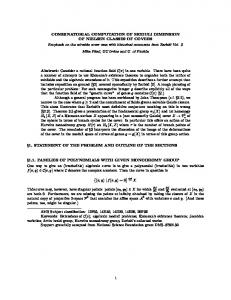
Figure 1.3. The fundamental domain of the P SL(2, Z)-action on the upper half plane H and the tiling of H by the P SL(2, Z)-orbits. Since the transformation T maps τ 7−→ τ + 1, the fundamental domain can be chosen as a subset of the vertical strip {τ ∈ H − 1/2 ≤ Re(τ ) < 1/2}. The transformation S : τ 7−→ −1/τ interchanges the inside and the outside of the semicircle |τ | = 1, Im(τ ) > 0. Therefore, we can choose the fundamental domain as in Figure 1.3. The arc of the semicircle from e2πi/3 to i is included in the fundamental domain, but the other side of the semicircle is not. Actually, S maps the left-side segment of the semicircle to the right-side, leaving i fixed. Note that the union [ H= A(Ω) A∈P SL(2,Z)

of the orbits of the fundamental domain Ω by all elements of P SL(2, Z) is not disjoint. Indeed, the point i is covered by Ω and S(Ω), and there are three regions that cover e2πi/3 . The quotient space H P SL(2, Z) is obtained by gluing the vertical line Re(τ ) = −1/2 with Re(τ ) = 1/2, and the left arc with the right arc. Thus the space looks like Figure 1.4.

10

MOTOHICO MULASE

i

e 2πi /3

Figure 1.4. The moduli space M1,1 . The moduli space M1,1 is an example of an orbifold, and in algebraic geometry, it is an example of an algebraic stack. It has two corner singularities. 1.3. Weierstrass Elliptic Functions. Let ω1 and ω2 be two nonzero complex numbers such that Im(ω1 /ω2 ) > 0. (It follows that ω1 and ω2 are linearly independent over the reals.) The Weierstrass elliptic function, or the Weierstrass ℘-function, of periods ω1 and ω2 is defined by (1.10) X 1 1 1 ℘(z) = ℘(z|ω1 , ω2 ) = 2 + − . z (z − mω1 − nω2 )2 (mω1 + nω2 )2 m,n∈Z (m,n)6=(0,0)

Let Λω1 ,ω2 = Z · ω1 + Z · ω2 be the lattice generated by ω1 and ω2 . If z ∈ / Λω1 ,ω2 , then the infinite sum (1.10) is absolutely and uniformly convergent. Thus ℘(z) is a holomorphic function defined on C \ Λω1 ,ω2 . To see the nature of the convergence of (1.10), fix an arbitrary z ∈ / Λω1 ,ω2 , and let N be a large positive number such that if |m| > N and |n| > N , then |mω1 + nω2 | > 2|z|. For such m and n, we have 1 |z| · |2(mω1 + nω2 ) − z| 1 (z − mω1 − nω2 )2 − (mω1 + nω2 )2 = |(z − mω1 − nω2 )2 (mω1 + nω2 )2 | |z| · 25 |mω1 + nω2 | 1 4 4 |mω1 + nω2 | 1 N

we have established the convergence of (1.10). At a point of the lattice Λω1 ,ω2 , ℘(z) has a double pole, as is clearly seen from its definition. Hence the Weierstrass elliptic function is globally meromorphic on C. From the definition, we can see that ℘(z) is an even function: (1.11)

℘(z) = ℘(−z).


11

Another characteristic property of ℘(z) we can read off from its definition (1.10) is its double periodicity: (1.12)

℘(z + ω1 ) = ℘(z + ω2 ) = ℘(z).

For example, ℘(z + ω1 ) 1 = + (z + ω1 )2 =

1 + (z + ω1 )2

X m,n∈Z (m,n)6=(0,0)

1 1 − 2 (z − (m − 1)ω1 − nω2 ) (mω1 + nω2 )2

X m,n∈Z (m,n)6=(0,0),(1,0)

X

+

m,n∈Z (m,n)6=(0,0),(1,0)

1 1 − 2 (z − (m − 1)ω1 − nω2 ) ((m − 1)ω1 + nω2 )2

1 1 − ((m − 1)ω1 + nω2 )2 (mω1 + nω2 )2

1 1 − 2 2 z ω 1 X

+

=

1 + z2

m,n∈Z (m,n)6=(1,0)

1 1 − 2 (z − (m − 1)ω1 − nω2 ) ((m − 1)ω1 + nω2 )2

= ℘(z). Note that there are no holomorphic functions on C that are doubly periodic, except for a constant. The derivative of the ℘-function, X 1 , (1.13) ℘0 (z) = −2 (z − mω1 − nω2 )3 m,n∈Z

is also a doubly periodic meromorphic function on C. The convergence and the periodicity of ℘0 (z) is much easier to prove than (1.10). Let us define two important constants: X 1 (1.14) g2 = g2 (ω1 , ω2 ) = 60 , (mω1 + nω2 )4 m,n∈Z (m,n)6=(0,0)

(1.15)

g3 = g3 (ω1 , ω2 ) = 140

X m,n∈Z (m,n)6=(0,0)

1 . (mω1 + nω2 )6

These are the most fundamental examples of the Eisenstein series. The combination ℘(z) − 1/z 2 is a holomorphic function near the origin. Let us calculate its Taylor expansion. Since ℘(z) − 1/z 2 is an even function, the expansion contains only even powers of z. From (1.10), the constant term of the expansion is 0. Differentiating it twice, four times, etc., we obtain 1 1 1 (1.16) ℘(z) = 2 + g2 z 2 + g3 z 4 + O(z 6 ). z 20 28 It follows from this expansion that 1 1 1 ℘0 (z) = −2 3 + g2 z + g3 z 3 + O(z 5 ). z 10 7

12

MOTOHICO MULASE

Let us now compare 1 2 1 4 − g2 2 − g3 + O(z 2 ), z6 5 z 7 3 1 3 1 4(℘(z))3 = 4 6 + g2 2 + g3 + O(z 2 ). z 5 z 7 It immediately follows that 1 (℘0 (z))2 − 4(℘(z))3 = −g2 2 − g3 + O(z 2 ). z Using (1.16) again, we conclude that (℘0 (z))2 = 4

def

f (z) = (℘0 (z))2 − 4(℘(z))3 + g2 ℘(z) + g3 = O(z 2 ). The equation means that (1) f (z) is a globally defined doubly periodic meromorphic function with possible poles at the lattice Λω1 ,ω2 ; (2) it is holomorphic at the origin, and hence holomorphic at every lattice point, too; (3) and it has a double zero at the origin. Therefore, we conclude that f (z) ≡ 0. We have thus derived the Weierstrass differential equation: (1.17)

(℘0 (z))2 = 4(℘(z))3 − g2 ℘(z) − g3 .

The differential equation implies that Z Z Z Z d℘ d℘ dz p d℘ = = . z = dz = 0 3 d℘ ℘ 4(℘) − g2 ℘ − g3 This last integral is called an elliptic integral. The Weierstrass ℘-function is thus the inverse function of an elliptic integral, and it explains the origin of the name elliptic function. Consider an ellipse x2 y2 + = 1, b > a > 0. a2 b2 From its parametric expression ( x = a cos(θ) y = b sin(θ), the arc length of the ellipse between 0 ≤ θ ≤ s is given by s Z s 2 2 Z sq dx dy (1.18) + dθ = b 1 − k 2 sin2 (θ)dθ, dθ dθ 0 0 where k 2 = 1 − a2 /b2 . This last integral is the Legendre-Jacobi second elliptic integral. Unless a = b, which is the case for the circle, (1.18) is not calculable in terms of elementary functions such as the trigonometric, exponential, and logarithmic functions. Mathematicians were led to consider the inverse functions of the elliptic integrals, and thus discovered the elliptic functions. The integral (1.18) can be immediately evaluated in terms of elliptic functions. The usefulness of the elliptic functions in physics was recognized soon after their discovery. For example, the exact motion of a pendulum is described by an elliptic


13

function. Unexpected appearances of elliptic functions have never stopped. It is an amazing coincidence that the Weierstrass differential equation implies that c u(x, t) = −℘(x + ct) + 3 solves the KdV equation 1 uxxx + 3uux , 4 giving a periodic wave solution traveling at the velocity −c. This observation was the key to the vast development of the 1980s on the Schottky problem and integrable systems of nonlinear partial differential equations called soliton equations [30]. ut =

1.4. Elliptic Functions and Elliptic Curves. A meromorphic function is a holomorphic map into the Riemann sphere P1 . Thus the Weierstrass ℘-function defines a holomorphic map from an elliptic curve onto the Riemann sphere: (1.19) ℘ : Eω1 ,ω2 = C Λω1 ,ω2 −−−−→ P1 = C ∪ {∞}. To prove that the map is surjective, we must show that the Weierstrass ℘-function C \ Λω1 ,ω2 −→ C is surjective. To this end, let us first recall Cauchy’s integral formula. Let ∞ X

an z n

n=−k

P be a power seires such that the sum of positive powers n≥0 an z n converges absolutely around the oriign 0 with the radius of convergence r > 0. Then for any positively oriented circle γ = {z ∈ C |z| = } of radius < r, we have I X ∞ 1 an z n = a−1 . 2πi γ n=−k

In this formulation, the integral formula is absolutely obvious. It has been generalized to the more familiar form that is taught in a standard complex analysis course. Let Ω be the parallelogram whose vertices are 0, ω1 , ω2 , and ω1 + ω2 . This is a fundamental domain of the Λω1 ,ω2 -action on the plane. Since the group acts by addition, the translation Ω + z0 of Ω by any number z0 is also a fundamental domain. Now, choose the shift z0 cleverly so that ℘(z) has no poles or zeros on the boundary γ of Ω + z0 . From the double periodicity of ℘(z) and ℘0 (z), we have I 0 I ℘ (z) d (1.20) dz = log ℘(z)dz = 0. ℘(z) dz γ γ This is because the integral along opposite sides of the parallelogram cancels. The function ℘0 (z) ℘(z) has a simple pole of residue m where ℘(z) has a zero of order m, and has a simple pole of residue −m where ℘(z) has a pole of order m. It is customary to count the number of zeros and poles with their multiplicity. Therefore, (1.20) shows that the number of poles and zeros of ℘(z) are exactly the same on the elliptic curve Eω1 ,ω2 . Since we know that ℘(z) has only one pole of order 2 on

14

MOTOHICO MULASE

the elliptic curve, it must have two zeros or a zero of order 2. Here we note that the formula (1.20) is also true for d log(℘(z) − c) dz for any constant c. This means that ℘(z) − c has two zeros or a zero of order 2. It follows that the map (1.19) is surjective, and its inverse image consists of two points, generically. Let e1 , e2 , and e3 be the three roots of the polynomial equation 4X 3 − g2 X − g3 = 0. Then except for the four points e1 , e2 , e3 , and ∞ of P1 , the map ℘ of (1.19) is two-to-one. This is because only at the preimage of e1 , e2 , and e3 the derivative ℘0 vanishes, and we know ℘ has a double pole at 0. We call the map ℘ of (1.19) a branched double covering of P1 ramified at e1 , e2 , e3 , and ∞. It is quite easy to determine the preimages of e1 , e2 and e3 via the ℘-function. Recall that ℘0 (z) is an odd function in z. Thus for j = 1, 2, we have ω ω ω ω j j j j − ωj = ℘0 − = ℘0 = −℘0 . ℘0 2 2 2 2 Hence ℘0

ω 1

2

= ℘0

ω 2

2

= ℘0

ω1 + ω2 2

= 0.

It is customary to choose the three roots e1 , e2 and e3 so that we have ω ω ω1 + ω2 1 2 (1.21) ℘ = e1 , ℘ = e2 , ℘ = e3 . 2 2 2 The quantities ω1 /2, ω2 /2, and (ω1 + ω2 )/2 are called the half periods of the Weierstrass ℘-function. The complex projective space Pn of dimension n is the set of equivalence classes of nonzero vectors (x0 , x1 , · · · , xn ) ∈ Cn+1 , where (x0 , x1 , · · · , xn ) and (y0 , y1 , · · · , yn ) are equivalent if there is a nonzero complex number c such that yj = cxj for all j. The equivalence class of a vector (x0 , x1 , · · · , xn ) is denoted by (x0 : x1 : · · · : xn ). We can define a map from an elliptic curve into P2 , (1.22) (℘, ℘0 ) : Eω1 ,ω2 = C Λω1 ,ω2 −−−−→ P2 , as follows: for Eω1 ,ω2 3 z 6= 0, we map it to (℘(z) : ℘0 (z) : 1) ∈ P2 . The origin of the elliptic curve is mapped to (0 : 1 : 0) ∈ P2 . In terms of the global coordinate (X : Y : Z) ∈ P2 , the image of the map (1.22) satisfies a homogeneous cubic equation (1.23)

Y 2 Z − 4X 3 + g2 XZ 2 + g3 Z 3 = 0.

The zero locus C of this cubic equation is a cubic curve, and this is why the Riemann surface Eω1 ,ω2 is called a curve. The affine part of the curve C is the locus of the equation Y 2 = 4X 3 − g2 X − g3 in the (X, Y )-plane and its real locus looks like Figure 1.5.


15

4 2

-1

-0.5

0.5

1

1.5

2

-2 -4

Figure 1.5. An example of a nonsingular cubic curve Y 2 = 4X 3 − g2 X − g3 . We note that the association   X = ℘(z) Y = ℘0 (z)   Z=1 is holomorphic for z ∈ C \ Λω1 ,ω2 , and provides a local holomorphic parameter of the cubic curve C. Thus C is non-singular at these points. Around the point (0 : 1 : 0) ∈ C ⊂ P2 , since Y 6= 0, we have an affine equation 3 2 3 Z X X Z Z −4 + g2 + g3 = 0. Y Y Y Y Y The association ( (1.24)

X Y Z Y

= =

℘(z) ℘0 (z) 1 ℘0 (z)

= − 12 z + O(z 5 ) = − 21 z 3 + O(z 7 ),

which follows from the earlier calculation of the Taylor expansions of ℘(z) and ℘0 (z), shows that the curve C near (0 : 1 : 0) has a holomorphic parameter z ∈ C defined near the origin. Thus the cubic curve C is everywhere non-singular. Note that the map z 7−→ (℘(z) : ℘0 (z) : 1) determines a bijection from Eω1 ,ω2 onto C. To see this, take an arbitrary point (X : Y : Z) on C. If it is the point at infinity, then (1.24) shows that the map is bijective near z = 0 because the relation can be solved for z = z(X/Y ) that gives a holomorphic function in X/Y . If (X : Y : Z) is not the point at infinity, then there are two points z and z 0 on Eω1 ,ω2 such that ℘(z) = ℘(z 0 ) = X/Z. Since ℘ is an even function, actually we have z 0 = −z. Indeed, z = −z as a point on Eω1 ,ω2 means 2z = 0. This happens exactly when z is equal to one of the three half periods. For a given value of X/Z, there are two points on C, namely (X : Y : Z) and (X : −Y : Z), that have the same X/Z. If (℘(z) : ℘0 (z) : 1) = (X : Y : Z), then (℘(−z) : ℘0 (−z) : 1) = (X : −Y : Z).

16

MOTOHICO MULASE

Therefore, we have (℘:℘0 :1)

Eω1 ,ω2 −−−−−→ bijection   ℘y

⊂

C −−−−→ P2   y

P1 P1 , where the vertical arrows are 2 : 1 ramified coverings. Since the inverse image of the 2 : 1 holomorphic mapping ℘ : Eω1 ,ω2 −→ P1 is ±z, the map ℘ induces a bijective map Eω1 ,ω2 {±1} −−−−−→ P1 . bijection

Because the group Z 2Z ∼ = {±1} acts on the elliptic curve Eω1 ,ω2 with exactly four fixed points ω2 ω1 + ω2 ω1 , , and , 0, 2 2 2 the quotient space Eω1 ,ω2 {±1} is not naturally a Riemann surface. It is P1 with orbifold singularities at e1 , e2 , e3 and ∞. 1.5. Degeneration of the Weierstrass Elliptic Function. The relation between the coefficients and the roots of the cubic polynomial 4X 3 − g2 X − g3 = 4(X − e1 )(X − e2 )(X − e3 ) reads   0 = e 1 + e 2 + e 3 g2 = −4(e1 e2 + e2 e3 + e3 e1 )   g3 = 4e1 e2 e3 . The discriminant of this polynomial is defined by 1 3 (g − 27g32 ). 16 2 We have noted that e1 , e2 , e3 , and ∞ are the branched points of the double covering ℘ : Eω1 ,ω2 −→ P1 . When the discriminant vanishes, these branched points are no longer separated, and the cubic curve (1.23) becomes singular. Let us now consider a special case ( ω1 = ri (1.25) ω2 = 1, 4 = (e1 − e2 )2 (e2 − e3 )2 (e3 − e1 )2 =

where r > 0 is a real number. We wish to investigate what happens to g2 (ri, 1), g3 (ri, 1) and the corresponding ℘-function as r → +∞. Actually, we will see the Eisenstein series degenerate into a Dirichlet series. The Riemann zeta function is a Dirichlet series of the form X 1 , Re(s) > 1. (1.26) ζ(s) = ns n>0 We will calculate its special values ζ(2g) for every integer g > 0 later. For the moment, we note some special values: ζ(2) =

π2 , 6

ζ(4) =

π4 , 90

ζ(6) =

π6 . 945


Since 1 g2 (ri, 1) = 60

X m,n∈Z (m,n)6=(0,0)

=2

17

1 (mri + n)4

X 1 X X X 1 1 1 + 2 + 2 + n4 (mr)4 (mri + n)4 (mri − n)4 m>0 m>0 n>0 n>0

= 2ζ(4) + 2

X (mri − n)4 + (mri + n)4 1 ζ(4) + 2 , 4 r ((mr)2 + n2 )4 m>0,n>0

we have an estimate X 2((mr)2 + n2 )2 1 1 60 g2 (ri, 1) − 2ζ(4) ≤ 2 r4 ζ(4) + 2 ((mr)2 + n2 )4 m>0,n>0 X 1 1 = 2 4 ζ(4) + 4 2 + n2 )2 r ((mr) m>0,n>0 X 1 1 < 2 4 ζ(4) + 4 2 r (mr) ((mr)2 + n2 ) m>0,n>0 X 1 1 < 2 4 ζ(4) + 4 r (mr)2 n2 m>0,n>0 =2

1 1 ζ(4) + 4 2 (ζ(2))2 . r4 r

Hence we have established lim g2 (ri, 1) = 120 ζ(4).

r→+∞

Similarly, we have 1 g3 (ri, 1) = 140

X m,n∈Z (m,n)6=(0,0)

1 (mri + n)6

= 2ζ(6) − 2

X 1 1 1 ζ(6) + 2 + r6 (mri + n)6 (mri − n)6 m,n>0

= 2ζ(6) − 2

X (mri − n)6 + (mri + n)6 1 ζ(6) + 2 , r6 ((mr)2 + n2 )6 m,n>0

hence X 2((mr)2 + n2 )3 1 < 2 1 ζ(6) + 2 g (ri, 1) − 2ζ(6) 3 140 r6 ((mr)2 + n2 )6 m,n>0 X 1 1 = 2 6 ζ(6) + 4 2 + n2 )3 r ((mr) m,n>0 0 (z − mri − n)2 (mri + n)2 n>0 n∈Z n∈Z XX 1 1 + − . (z − mri − n)2 (mri + n)2 m0 n∈Z n∈Z X X X 1 1 + − 2 2 (z − mri − n) (mri + n) m0 X π2 π2 + − sin2 (πz − πmri) sin2 (πmri) m0 X X π2 π2 + + . 2 2 | sin (πz − πmri)| m0 m>0 Z ∞ 1 dx < + 2 sinh2 (πr) sinh (πrx) 1 1 coth(πr) − 1 + −→ 0. = r→∞ πr sinh2 (πr)


19

The same is true for m < 0. To establish an estimate of the terms that are dependent on z = x + iy, let us impose the following restrictions: r r (1.27) 0 ≤ Re(z) = x < 1, − < Im(z) = y < . 2 2 ri

r ri+n

1

Figure 1.6. Degeneration of a lattice to the integral points on the real axis. Since all functions involved have period 1, the condition for the real part is not a restriction. We wish to show that X π2 lim =0 2 r→∞ | sin (πz − πmri)| m>0 uniformly on every compact subset of (1.27). X X 1 4 = 2 πiz πmr − e−πiz e−πmr |2 | sin (πz − πmri)| m>0 |e e m>0 X 4 = e−2πmr πiz −πiz e−2πmr |2 |e − e m>0 X 4 ≤ e−2πmr −πy πy e−2πmr )2 (e − e m>0 X 4 < e−2πmr −πy (e − e−πr )2 m>0 =

e−2πr 4 · −→ 0. 1 − e−2πr (e−πy − e−πr )2 r→∞

A similar estimate holds for m < 0. We have thus established the convergence lim ℘(z|ri, 1) =

r→∞

π2 − 2 ζ(2). sin (πz) 2

Let f (z) denote this limiting function, g2 = 120 ζ(4), and g3 = 280 ζ(6). Then, as we certainly expect, the following differential equation holds: 2 2π 2 π2 (f 0 (z))2 = 4f (z)3 − g2 f (z) − g3 = 4 f (z) − · f (z) + . 3 3 Geometrically, the elliptic curve becomes an infinitely long cylinder, but still the top circle and the bottom circle are glued together as one point. It is a singular

20

MOTOHICO MULASE

algebraic curve given by the equation 2 2π 2 π2 Y2 =4 X − . · X+ 3 3 We note that at the point (−π 2 /3, 0) of this curve, we cannot define the unique tangent line, which shows that it is a singular point. 1.6. The Elliptic Modular Function. The Eisenstein series g2 and g3 depend on both ω1 and ω2 . However, the quotient (1.28)

J(τ ) =

g2 (ω1 , ω2 )3 ω212 g2 (τ, 1)3 = · g2 (ω1 , ω2 )3 − 27g3 (ω1 , ω2 )2 ω212 g2 (τ, 1)3 − 27g3 (τ, 1)2

is a function depending only on τ = ω1 /ω2 ∈ H. This is what is called the elliptic modular function. From its definition it is obvious that J(τ ) is invariant under the modular transformation aτ + b τ 7−→ , cτ + d a b where ∈ P SL(2, Z). Since the Eisenstein series g2 (τ, 1) and g3 (τ, 1) are c d absolutely convergent, J(τ ) is complex differentiable with respect to τ ∈ H. Hence J(τ ) is holomorphic on H, except for possible singularities coming from the zeros of the discriminant g23 − 27g32 . However, we have already shown that the cubic curve (1.23) is non-singular, and hence g23 − 27g32 6= 0 for any τ ∈ H. Therefore, J(τ ) is indeed holomorphic everywhere on H. To compute a few values of J(τ ), let us calculate g3 (i, 1). First, let Λ = {mi + n m ≥ 0, n > 0, (m, n) 6= (0, 0)}. Since the square lattice Λi,1 has 90◦ rotational symmetry, it is partitioned into the disjoint union of the following four pieces: Λi,1 \ {0} = Λ ∪ iΛ ∪ i2 Λ ∪ i3 Λ.

i 1

Figure 1.7. A partition of the square lattice Λi,1 into four pieces. Thus we have 1 g3 (i, 1) = 140

X m,n∈Z (m,n)6=(0,0)

1 (mi + n)6


=

1+

1 1 1 + 12 + 18 6 i i i

21

X m≥0,n>0 (m,n)6=(0,0)

1 (mi + n)6

=0. Similarly, let ω = eπi/3 . Since ω 6 = 1, the honeycomb lattice Λω,1 has 60◦ rotational symmetry. Let L = {mω + n m ≥ 0, n > 0, (m, n) 6= (0, 0)}. Due to the 60◦ rotational symmetry, the whole honeycomb is divided into the disjoint union of six pieces: Λω,1 \ {0} = L ∪ ωL ∪ ω 2 L ∪ ω 3 L ∪ ω 4 L ∪ ω 5 L.

ω 1

Figure 1.8. A partition of the honeycomb lattice Λω,1 into six pieces. Therefore, 1 g2 (ω, 1) = 60

X m,n∈Z (m,n)6=(0,0)

=

1+

1 (mω + n)4

1 1 1 1 1 + 8 + 12 + 16 + 20 ω4 ω ω ω ω

= (1 + ω 2 + ω 4 + 1 + ω 2 + ω 4 )

X m≥0,n>0 (m,n)6=(0,0)

X m≥0,n>0 (m,n)6=(0,0)

1 (mω + n)4

1 (mω + n)4

= 0. We have thus established g2 (i, 1)3 = 1, g2 (i, 1)3 − 27g3 (i, 1)2 g2 (ω, 1)3 J(e2πi/3 ) = J(ω) = = 0. g2 (ω, 1)3 − 27g3 (ω, 1)2 J(i) =

(1.29)

Moreover, we see that J(τ ) − 1 has a double zero at τ = i, and J(τ ) has a triple zero at τ = e2πi/3 . This is consistent with the fact that i and e2πi/3 are the fixed points of the P SL(2, Z)-action on H, with an order 2 stabilizer subgroup at i and an order 3 stabilizer subgroup at e2πi/3 .

22

MOTOHICO MULASE

Another value of J(τ ) we can calculate is the value at the infinity i∞: g2 (ri, 1)3 = ∞. r→+∞ g2 (ri, 1)3 − 27g3 (ri, 1)2

J(i∞) = lim J(ri) = lim r→+∞

The following theorem is a fundamental result. Theorem 1.12 (Properties of J).

(1) The elliptic modular function J : H −→ C

is a surjective holomorphic function which defines a bijective holomorphic map (1.30) H P SL(2, Z) ∪ {i∞} −→ P1 . (2) Two elliptic curves Eτ and Eτ 0 are isomorphic if and only if J(τ ) = J(τ 0 ). Remark. The bijective holomorphic map (1.30) is not biholomorphic. Indeed, as √ −1 3 z at z = 0 ∈ P1 , and we have already observed, the expansion of J starts with √ starts with z − 1 at z = 1. From this point of view, the moduli space M1,1 is not isomorphic to C. In order to prove Theorem 1.12, first we parametrize the structure of an elliptic curve Eτ in terms of the branched points of the double covering ℘ : Eτ −→ P1 . We then re-define the elliptic modular function J in terms of the branched points. The statements follow from this new description of the modular invariant. Let us begin by determining the holomorphic automorphisms of P1 . Since P1 = C2 \ (0, 0) C× , where C× = C\{0} is the multiplicative group of complex numbers, we immediately see that P GL(2, C) = GL(2, C) C× is a subgroup of Aut(P1 ). In terms of the coordinate z of P1 = C ∪ {∞}, the P GL(2, C)-action is described again as linear fractional transformation: az + b a b (1.31) ·z = . c d cz + d Let f ∈ Aut(P1 ). Since (1.31) can bring any point z to ∞, by composing f with a linear fractional transformation, we can make the automorphism fix ∞. Then this automorphism is an affine transformation, since it is in Aut(C). Therefore, we have shown that Aut(P1 ) = P GL(2, C). We note that the linear fractional transformation (1.31) brings 0, 1, and ∞ to the following three points:  0 7−→ db  1 7−→ a+b c+d   ∞ 7−→ ac .


23

Since the only condition for a, b, c and d is ad−bc 6= 0, it is easy to see that 0, 1 and ∞ can be brought to any three distinct points of P1 . In other words, P GL(2, C) acts on P1 triply transitively. Now consider an elliptic curve E defined by a cubic equation Y 2 Z = 4X 3 − g2 XZ 2 − g3 Z 3 in P2 , and the projection to the X-coordinate line ( (X : Y : Z) 7−→ (X : Z) ∈ P1 p:E3 (0 : 1 : 0) 7−→ (1 : 0) ∈ P1 .

Z 6= 0,

Note that we are assuming that g23 − 27g32 6= 0. As a coordinate of P1 , we use x = X/Z. As before, let 4x3 − g2 x − g3 = 4(x − e1 )(x − e2 )(x − e3 ). Then the double covering p is ramified at e1 , e2 , e3 and ∞. Since these four points are distinct, we can bring three of them to 0, 1, and ∞ by an automorphism of P1 . The fourth point cannot be brought to a prescribed location, so let λ be the fourth branched point under the action of this automorphism. In particular, we can choose e3 − e2 (1.32) λ= . e3 − e1 This is the image of e3 via the transformation x − e2 x 7−→ . x − e1 This transformation maps  e1 7−→ ∞    e 7−→ 0 2  e3 7−→ λ    ∞ 7−→ 1 . Noting the relation e1 + e2 + e3 = 0, a direct calculation shows g23 − 27g32 −64(e1 e2 + e2 e3 + e3 e1 )3 = 16(e1 − e2 )2 (e2 − e3 )2 (e3 − e1 )2 3 − 3(e1 e2 + e2 e3 + e3 e1 ) 4 = 27 (e1 − e2 )2 (e2 − e3 )2 (e3 − e1 )2

J(τ ) =

g23

3 4 (e1 + e2 + e3 )2 − 3(e1 e2 + e2 e3 + e3 e1 ) = 27 (e1 − e2 )2 (e2 − e3 )2 (e3 − e1 )2 3 4 e21 + e22 + e23 − (e1 e2 + e2 e3 + e3 e1 ) = 27 (e1 − e2 )2 (e2 − e3 )2 (e3 − e1 )2 3 4 (e3 − e2 )2 − (e3 − e2 )(e3 − e1 ) + (e3 − e1 )2 ) = 27 (e1 − e2 )2 (e2 − e3 )2 (e3 − e1 )2 2 4 (λ − λ + 1)3 = . 27 λ2 (λ − 1)2

24

MOTOHICO MULASE

Of course naming the three roots of the cubic polynomial is arbitrary, so the definition of λ (1.32) receives the action of the symmetric group S3 . We could have chosen any one of the following six choices as our λ: e3 − e2 , e3 − e1 λ e2 − e3 = , λ−1 e2 − e1 λ=

(1.33)

1 e3 − e1 1 e2 − e1 = , 1− = , λ e3 − e2 λ e2 − e3 e1 − e2 1 e1 − e3 1−λ= , = . e1 − e3 1−λ e1 − e2

Since the rational map (1.34)

µ = j(λ) =

4 (λ2 − λ + 1)3 27 λ2 (λ − 1)2

is a symmetric function of e1 , e2 , e3 , it has the same value for any of the six choices (1.33). The rational map j has degree 6, and hence the inverse image j −1 (µ) of µ ∈ C exactly coincides with the 6 values given above. The value j(λ) of the elliptic curve is called the j-invariant. Lemma 1.13. Let E (resp. E 0 ) be an elliptic curve constructed as a double covering of P1 ramified at 0, 1, ∞, and λ (resp. λ0 ). Suppose j(λ) = j(λ0 ). Then E and E 0 are isomorphic. Proof. Since j : P1 −→ P1 is a ramified covering of degree 6, j(λ) = j(λ0 ) implies that λ0 is one of the 6 values listed in (1.33). Now let us bring back the four ramification points 0, 1, ∞, and λ to e1 , e2 , e3 , and ∞ by solving two linear equations (1.35)

λ=

e3 − e2 e3 − e1

and

e1 + e2 + e3 = 0.

The solution is unique up to an overall constant factor, which does not affect the value g3 4 (λ2 − λ + 1)3 = 3 2 2. j(λ) = 2 2 27 λ (λ − 1) g2 − 27g3 We also note that (e1 , e2 , e3 ) and their constant multiple (ce1 , ce2 , ce3 ) define an isomorphic elliptic curve. So choose a particular solution e1 , e2 and e3 of (1.35). Then the difference between λ and λ0 is just a permutation of e1 , e2 and e3 . In particular, the defining cubic equation of the elliptic curve, which is symmetric under permutation of e1 , e2 and e3 , is exactly the same. Thus E and E 0 are isomorphic. We are now ready to prove Theorem 1.12. Proof. First, take an arbitrary µ ∈ C, and let λ be a point in the inverse image of µ via the map j. We can construct a cubic curve E as a double cover of P1 ramified at 0, 1, ∞, and λ. Since it is a Riemann surface of genus 1, it is isomorphic to a particular elliptic curve Eτ for some τ ∈ H. Realize Eτ as a cubic curve, and choose its ramification points 0, 1, ∞, and λ0 . Here we have applied an automorphism of P1 to choose this form of the ramification point. Since E and Eτ are isomorphic, we have J(τ ) = j(λ0 ) = j(λ) = µ.


25

This establishes that J : H −→ C is surjective. We have already established that J(τ ) = J(τ 0 ) implies the isomorphism Eτ ∼ = Eτ 0 , by translating the equation into λ-values. This fact also shows that the map J : H P SL(2, Z) −→ C is one-to-one. We have shown that J(i∞) = ∞, but we have not seen how the modular function behaves at infinity. This is our final subject of this section, which completes the proof of Theorem 1.12. ir

D

γ

i

E

C

B A

F

0

1

Figure 1.9. The boundary of the fundamental domain as an integration contour. Let γ be the contour defined in Figure 1.9. It is the boundary of a fundamental _

domain of the P SL(2, Z)-action, except for an arc AB, a line segment CD, and _ another arc EF . Since J : H P SL(2, Z) −→ C is a bijective holomorphic map, and since J(e2πi/3 ) = 0, J does not have any other zeros in the fundamental domain. Therefore, d log J(τ ) is holomorphic everywhere inside the contour γ, and we have I d log J(τ ) = 0. γ

By differentiating the equation J(τ ) = J (aτ + b)/(cτ + d) , we obtain 1 aτ + b 0 0 J (τ ) = J . cτ + d (cτ + d)2 Hence 0

0

dJ(τ ) = J (τ )dτ = J aτ + b = dJ . cτ + d

aτ + b cτ + d

1 dτ = J 0 (cτ + d)2

aτ + b cτ + d

aτ + b d cτ + d

26

MOTOHICO MULASE

(The exterior differentiation d and the integer d should not be confused.) It follows that aτ + b d log J(τ ) = d log J . cτ + d Therefore, we have Z

C

Z

E

d log J(τ ) + B Z i

d log J(τ ) = 0

Z d log J(τ ) +

F

D A

d log J(τ ) = 0. i

Next, since J(e2πi/3 ) = 0 is a zero of order 3, the integral of d log J(τ ) around e2πi/3 is given by I d log J(τ ) = 6πi. _

_

The arcs AB and EF joined together form a third of a small circle going around e2πi/3 clockwise. Therefore, we have Z B Z F I 1 d log J(τ ) + d log J(τ ) = − d log J(τ ) = −2πi. 3 A E Thus we are left with the integration along the line segment CD. In order to study the behavior of J(τ ) as τ −→ i∞, we introduce a new varialbe q = e2πiτ . Since J(τ + 1) = J(τ ), the elliptic modular function admits a Fourier series expansion in terms of q = e2πiτ . So let f (q) = f (e2πiτ ) = J(τ ) be the Fourier expansion of J(τ ). Note that J 0 (τ ) f 0 (q) dτ = d log J(τ ) = d log f (q) = dq. J(τ ) f (q) The points C = 1/2+ir and D = −1/2+ir in τ -coordinate transform into eπi e−2πr and e−πi e−2πr in q-coordinate, respectively. Therefore, the path CD is a loop of radius e−2πr around q = 0 with the counter clockwise orientation in q-coordinate. Thus we have Z D Z e−πi e−2πr I d log J(τ ) = d log f (q) = − d log f (q) = 2πin, eπi e−2πr

C

where n is the order of the pole of f (q) at q = 0. Altogether, we have established I 0= d log J(τ ) = 2πin − 2πi = 2πi(n − 1). γ

Therefore, we conclude n = 1. Hence f (q) has a simple pole at q = 0, or τ = i∞. In other words, the map J : H P SL(2, Z) ∪ {i∞} −→ P1 is holomorphic around the point i∞. This completes the proof of Theorem 1.12.


27

The first few terms of the q-expansion of J(τ ) are given by 1 J(τ ) = (q −1 + 744 + 196884q + 21493760q 2 + · · · ). 1728 We refer to [9] for the story of these coefficients, the Monstrous Moonshine, and its final mathematical outcome. 1.7. Compactification of the Moduli of Elliptic Curves. We have introduced two different ways to parametrize the moduli space M1,1 of elliptic curves. The first one is through the period τ ∈ H of an elliptic curve, and the other via the fourth ramification point λ ∈ P1 \ {0, 1, ∞} when we realize an elliptic curve as a double cover over P1 ramified at 0, 1, ∞ and λ. The equality we have proven, J(τ ) =

4 λ2 − λ + 1 g2 (τ, 1)3 = , g2 (τ, 1)3 − 27g3 (τ, 1)2 27 λ2 (1 − λ)2

gives two holomorphic fibrations over C: P1 \ {0, 1, ∞}   j yS3 -action

(1.36) J

H −−−−−−−−−−→ P SL(2,Z)-action

C.

We have also established that the function j(λ) is invariant under the action of S3 , and the elliptic modular function J(τ ) is invariant under the action of the modular group P SL(2, Z). It is intriguing to note the similarity of these two groups. In the presentation by generators and their relations, we have P SL(2, Z) = hS, T S 2 = (ST )3 = 1i, (1.37) S3 = hs, t s2 = t2 = (st)3 = 1i. Therefore, there is a natural surjective homomorphism (1.38)

h : P SL(2, Z) −→ S3

defined by h(S) = s and h(T ) = t. The kernel Ker(h) is a normal subgroup of P SL(2, Z) of index 6. Proposition 1.14 (Congruence subgroup modulo 2). The kernel Ker(h) of the homomorphism h : P SL(2, Z) −→ S3 is equal to the congruence subgroup of P SL(2, Z) modulo 2: a b a b 1 0 Ker(h) = Γ(2) = ∈ P SL(2, Z) ≡ mod 2 . c d c d 0 1 def In particular, we have an isomorphism P SL(2Z) Γ(2) ∼ = S3 . Proof. Let 1 A=T = 0

2 , 1 1 0 −2 B = ST S = . 2 1 2

28

MOTOHICO MULASE

Obviously A and B are elements of both Ker(h) and Γ(2). First let us show that A and B generate Γ(2): Γ(2) = hA, Bi. The condition ad − bc = 1 means that a and b are relatively prime, and the congruence condition a b 1 0 ≡ mod 2 c d 0 1 means that a and d are odd and and c are even. Since the multiplication of the b a b n matrix A from the right to changes b to 2na + b, by a suitable choice of c d the power n, we can make |b| < |a|. (They cannot be equal because a is odd and b is even.) On the other hand, the multiplication of B m from the right changes a to a + 2mb. Thus by a suitable choice of the power of B, we can make |a| < |b|. Hence by consecutive multiplications of suitable powers of A and B from the right, a b 1 b0 ∈ Γ(2) is brought to the form 0 , which is still an element of Γ(2). c d c d0 −b0 /2 Thus b0 is even, and from the right brings the hence further application of A 1 0 matrix to 0 . The determinant condition dictates that ∗ = 1. Since c0 is c ∗ 0 1 0 also even, 0 = B c /2 . Hence Γ(2) is generated by A and B. In particular, c 1 Γ(2) ⊂ Ker(h). Next let us determine the index of Γ(2) in P SL(2Z). The method of exhaustive listing works here. As a representative of the coset P SL(2Z) Γ(2), we can choose 1 0 1 1 1 0 0 −1 1 −1 0 −1 , , , , , . 0 1 0 1 1 1 1 0 1 0 1 1 Therefore, Γ(2) is an index 6 subgroup of P SL(2Z). It implies that Γ(2) = Ker(h). This completes the proof. Figure 1.10 shows a fundamental domain of the Γ(2)-action on the upper half plane H. We observe that the line Re(τ ) = −1 is mapped to the line Re(τ ) = 1 by and 0 is mapped to the A = T 2 ∈ Γ(2), and the semicircle connecting −1, −1+i 2 −2 semicircle connecting 1, 1+i and 0 by B = ST S ∈ Γ(2). Gluing these dotted 2 lines and semicircles, we obtain a sphere minus three points. Because of the triple transitivity of Aut(P1 ), we know that M0,3 consists of only one point: (1.39) M0,3 = P1 , (0, 1, ∞) . Therefore, we can identity H Γ(2) ∼ = P1 \ {0, 1, ∞}. We now have a commutative diagram that completes (1.36).

(1.40)

H

Γ(2)-action

−−−−−−−→

J

H −−−−−−−−−−→ P SL(2,Z)-action

P1 \ {0, 1, ∞}   j yS3 -action P1 \ {∞}.


29

i

−2

−1

0

1

2

Figure 1.10. A fundamental domain of the action of the congruence subgroup Γ(2) ⊂ P SL(2, Z). Let us study the geometry of the map j : P1 3 λ 7−→

4 (λ2 − λ + 1)3 ∈ P1 . 27 λ2 (1 − λ)2

We see that j −1 (∞) = {0, 1, ∞}, and that each of the three points has multiplicity 2. To see the ramification of j at 0 and 1, let us consider the inverse image of the closed real interval [0, 1] on the target P1 via j. Figure 1.11 shows j −1 ([0, 1]). The shape is the union of two circles of radius 1 centered at 0 and 1, intersecting at eπi/3 and e−πi/3 with a 120◦ angle. The inverse image j −1 ([0, 1]) also contains the vertical line segment eπi/3 e−πi/3 . Each point of j −1 (∞) = {0, 1, ∞} is surrounded by a bigon, representing the fact that the ramification at each point is of degree 2. Each point of j −1 (0) = {eπi/3 , e−πi/3 } has multiplicity 3, which can be seen by the tri-valent vertex of the graph j −1 ([0, 1]) at eπi/3 and e−πi/3 . And finally, each point of j −1 (1) = {−1, 12 , 2} has multiplicity 2 and is located at the middle of an edge of the graph. 1

0.5

-1

-0.5

0.5

1

1.5

2

-0.5

-1

Figure 1.11. The inverse image of [0, 1] via the map j(λ) = 4 λ2 −λ+1 27 λ2 (1−λ)2 . (Graphics produced by Josephine Yu.) More geometrically, consider P1 as a sphere with its real axis as the equator, and ω = eπi/3 and ω −1 = e−πi/3 as the north and the south poles. Then we can see that the S3 -action on P1 is equivalent to the action of the dihedral group D3 on the

30

MOTOHICO MULASE

πi/3 equilateral triangle 401∞. It becomes obvious that and ω −1 = e−πi/3 ω=e are stabilized by the action of the cyclic group Z 3Z through the 120◦ rotations about the axis connecting the poles, and each of 0, 1, ∞ and −1, 12 , 2 is invariant under the 180◦ rotation about a diameter of the equator. ω

∞

−1

2

0

1

_1 2

ω−1

Figure 1.12. The S3 -action on P1 through the dihedral group action. Since the P SL(2, Z)-action on H factors through the Γ(2)-action and the S3 action, we have the equality 1 M1,1 = H P SL(2, Z) = H Γ(2) S3 = P \ {0, 1, ∞} S3 . At this stage, we can define a compactification of the moduli space M1,1 by (1.41) M1,1 = P1 S3 . Since S3 acts on P1 properly discontinuously, the quotient is again an orbifold. The stabilizer subgroup at eπi/3 is Z 3Z, and the stabilizer subgroup at 21 is Z 2Z. Therefore, the orbifold structure of P1 S3 at its singular points j = 0 and j = 1 is exactly the same as we have observed before. (We refer to Chapter ?? for the definition of orbifolds and the terminology from the orbifold theory.) However, there is a big difference in the singularity structure at ∞. From (1.41), the compactified moduli space has the quotient singularity modeled by the Z 2Zaction on P1 at ∞. On the other hand, as we have seen in the last section, the elliptic modular function J(τ ) has a simple pole at q = 0 in terms of the variable q = e2πiτ . This shows that the moduli space has a compactification J M1,1 = H P SL(2Z) ∪ {i∞} −−−−−−−−−−−−−−−−→ C ∪ {∞} = P1 , holomorphic and bijective

−1

and that J is a holomorphic map at ∞ ∈ P1 . How do we reconcile this difference? This is due to the fact that the upper half plane H, which is isomorphic to the unit open disk {z ∈ C |z| < 1} by the Riemann mapping theorem, does not have any natural compactification as a Riemann surface. Therefore we cannot take the compactification of H before taking the quotient by the modular group P SL(2, Z). The point {i∞}, called the cusp point, is added only after taking the full quotient. But if we take another route by first constructing the quotient by a normal subgroup such as the congruence subgroup Γ(2), then we can


31

add three points to compactify the quotient space. The moduli space in question is the quotient of this intermediate quotient space by the action of the factor group P SL(2, Z) Γ(2) = S3 . In this second construction, we end up with a compact orbifold with a singularity at ∞. The moduli space M1,1 is an infinite cylinder near ∞. Therefore, depending on when we compactify it, the point at infinity can be an orbifold singularity modeled by any Z nZ-action on the complex plane. Thus we note that the moduli space M1,1 does not have a canonical orbifold compactification. The point at infinity can be added as a non-singular point, or as a Z 2Z-singular point, or in many other different ways. We also note that if we wish to consider the compactified moduli space of elliptic curves as an algebraic variety, then the natural identification is M1,1 ∼ = P1 without any singularities. Its complex structure is introduced by the modular function J(τ ). For a higher genus, the situation becomes far more complex. Compactification of Mg,n as an algebraic variety is no longer unique, and compactification as an orbifold is even more non-unique. In the later chapters, we consider the canonical orbifold structure of the non-compact moduli space Mg,n . It is still an open question to find an orbifold compactification of Mg,n with an orbifold cell-decomposition that restricts to the canonical orbifold cell-decomposition of the moduli space. 2. Matrix Integrals and Feynman Diagram Expansion This chapter is devoted to the study of the asymptotic analysis of various matrix integrals. We investigate symmetric, Hermitian, and quarternionic self-adjoint matrices separately. These integrals can be thought of as 0-dimensional models of Quantum Field Theory. QFT produces many interesting and useful mathematical tools. In this chapter, we deal with QFT as a machinery of counting formula. QFT provides us with a clever method of counting the order of certain finite groups. Often QFT is not well-defined mathematically, but all our models lead to finite dimensional integrals and therefore they are well-defined. We will develop two different methods for calculating some of the QFT integrals. Since the original integral is well-defined, the two methods should provide the same answer. This apparent equality turns out to be an interesting equality in mathematics. Let us begin by reviewing asymptotic analysis of holomorphic functions. 2.1. Asymptotic Expansion of Analytic Functions. A holomorphic function admits a convergent Taylor series expansion at each point of the domain of definition. What happens if we try to expand the function into a power series at a boundary point of the domain? We investigate this question in this section. Since our goal is the asymptotic analysis of matrix integrals, we focus our study on the techniques used in matrix integrals, instead of developing the most general theory of asymptotic series. When we are first introduced to complex analysis, perhaps the most surprizing thing may have been the fact that complex differentiability implies complex analyticity. Let h(z) be a continuous function defined on an open domain U ⊂ C. If h(z) is continuously differentiable everywhere in U , then it satisfies Cauchy’s Theorem

32

MOTOHICO MULASE

of Integration: I h(z)dz = 0, γ

where γ is a closed loop in U . One can then show that h(z) satisfies the Cauchy Integral Formula I 1 h(z) (2.1) h(w) = dz, 2πi γ z − w where γ is a simple loop in U that goes around w ∈ U once counter-clockwise. But (2.1) immediately implies that h(z) has Taylor expansion everywhere in U . What happens if h(z) is continuously differentiable not on an entire neighborhood of a point, say 0, but only a part of the neighborhood? This motivates us to introduce the following definition. Definition 2.1 (Asymptotic Expansion). Let h be a holomorphic function defined on a wedge-shaped domain Ω: Ω = {z ∈ C α < arg(z) < β, |z| < r.} P A power series n≥0 an z n is said to be an asymptotic expansion of h at the origin 0 ∈ ∂Ω if Pm−1 h(z) − n=0 an z n = am (2.2) lim z→0 zm z∈Ω

holds for every m ≥ 0. When an asymptotic expansion exists, we say h has an asymptotic expansion on Ω at its boundary point 0.

Ω β α 0

Figure 2.1. A wedge-shaped domain. Let us examine the implications of (2.2). For m = 0, it requires the convergence of h(z) as t −→ 0 while in Ω. Thus h(z) is continuous at 0 when approaching from inside Ω. We can define the value of h(z) at 0 by h(0) = a0 . For m = 1, the existence of h(z) − h(0) lim = a1 z→0 z z∈Ω

implies that h(z) is differentiable at 0 when approaching from inside Ω. Let us call the situation Ω-differentiable. Since h(z) is holomorphic on Ω, we can differentiate the numerator and the denominator of (2.2) (m−1)-times and obtain the same limit. The existence of the limit Pm−1 h(z) − n=0 an z n h(m−1) (z) − (m − 1)!am−1 lim = lim = am z→0 z→0 zm m!z z∈Ω

z∈Ω


33

thus implies that h(m−1) (z) is Ω-differentiable, and that h(m) (0) = m!am . Therefore, the existence of an asymptotic expansion at 0 ∈ Ω simply means the function h(z) is infinitely many times continuously Ω-differentiable at 0. The above consideration immediately implies Proposition 2.2 (Uniqueness of asymptotic expansion). If a holomorphic function h on Ω has an asymptotic expansion at 0 ∈ ∂Ω as above, then it is unique. The simplest example of an asymptotic expansion is the Taylor expansion when h is holomorphic at 0. Since h is infinitely many times continuously differentiable in a neighborhood of 0, h(m) (0) is well-defined for all m ≥ 0, and the Taylor expansion h(z) =

X h(m) (0) zm m!

n≥0

gives the asymptotic expansion of h(z) at z = 0. The technique of asymptotic expansion is developed to study the behavior of a holomorphic function at its essential singularity. When a holomorphic function h(z) has an essential singularity at 0, often we can find a wedge-shaped domain Ω with 0 as its vertex such that the function is infinitely many times continuously differentiable on Ω. We can then expand the function into its asymptotic series and study its properties. The existence of such a domain is significant because h(z) can take arbitrary values except for up to two excluded values in any neighborhood of 0 (Picard’s Theorem). If h is defined on a larger domain Ω0 that contains Ω and has an asymptotic expansion on Ω0 , then h has an asymptotic expansion also on Ω and the asymptotic series are exactly the same. In general, however, the existence depends on the choice of the domain Ω. Example 2.1. Consider h(z) = e1/z . It is holomorphic on C \ {0}. If we choose π 3π + < arg(z) < − }, 2 2 then it has an asymptotic expansion on Ω at 0, and its asymptotic series is the zero series. However, if we choose a wedge-shaped domain contained in the right half plane Re(z) > 0, then e1/z does not have any asymptotic expansion. (2.3)

Ω = {z ∈ C |

This example also shows that two different holomorphic functions may have the same asymptotic expansion on the same domain. P From this point of view, the holomorphic function h and its asymptotic series n≥0 an z n are not equal. We use the notation X (2.4) A(h) = an z n n≥0

to indicate that the series of the right hand side is the asymptotic expansion of h(z). We also use h(z) ≡ g(z) if h(z) and g(z) have the same asymptotic expansion on the same domain. Thus 0 ≡ e1/z on the domain of (2.3). Proposition 2.3 (Properties of the asymptotic expansion). Let f (z) and h(z) be holomorphic functions on a domain Ω and have asymptotic expansions at its

34

MOTOHICO MULASE

boundary point 0 ∈ ∂Ω: A(f ) =

X

an z n ,

A(h) =

X

bn z n .

n≥0

n≥0

Then (2.5)

A(f + h) = A(f ) + A(h)

(2.6)

A(f · h) = A(f ) · A(h)

Proof. For every m ≥ 0, we have Pm−1 Pm−1 f (z) + h(z) − n=0 (an + bn )z n f (z) − n=0 an z n lim = lim zm zm Pm−1 h(z) − n=0 bn z n + lim zm = am + bm . This proves (2.5). Since we know lim and lim

f (z)

f (z)h(z) − f (z) zm

Pm−1 k=0

bk z k −

Pm−1 n=0

Pm−1 n=0 zm

an z n

bk z k

= a0 bm

Pm−1 k=0

bk z k

= am b0 ,

adding the above two equations, we have Pm−1 Pm−1 f (z)h(z) − n=0 an z n k=0 bk z k = a0 bm + am b0 . lim zm Note that m−1 X

an z n

n=0

m−1 X

bk z k

k=0

=

X

an bk z n+k + (a1 bm−1 + a2 bm−2 + · · · am−1 b1 )z m + O(z m+1 ).

n+k≤m−1

Therefore, we obtain lim This proves (2.6).

f (z)h(z) −

P

n+k≤m−1 zm

an bk z n+k

=

X

an bk .

n+k=m

Let us now consider a simple example Z +∞ t 4 1 2 1 e− 2 x e 4! x dx. Z4 (t) = √ 2π −∞ The integral Z4 (t) is a holomorphic function in t for Re(t) < 0 and continuous for Re(t) ≤ 0. Let Ω = {t ∈ C | 2π/3 < arg(t) < 4π/3}. We wish to find the asymptotic expansion of Z4 on Ω at t = 0. First we note that if t ∈ Ω, then t 4 Re(t) 4 4! x e = e 4! x ≤ 1.


35

We claim: X A Z4 (t) =

(2.7)

n≥0

tn (4!)n n!

1 √ 2π

Z

+∞

1 2 e− 2 x x4n dx .

−∞

Indeed, we have ! Z +∞ m−1 X tn Z +∞ 1 2 t 4 1 x − 21 x2 4! − 2 x 4n lim e e dx − e x dx t→0 tm (4!)n n! −∞ −∞ n=0 t∈Ω   Z +∞ Z +∞ m−1 n n X X 1 2 1 2 1 t t e− 2 x x4n dx − x4n dx = lim m  e− 2 x n n! n n! t→0 t (4!) (4!) −∞ −∞ n=0 n≥0

t∈Ω

∞ X

+∞ 1 2 1 tn e− 2 x x4n dx m n n! t→0 t (4!) −∞ n=m t∈Ω Z +∞ ∞ X 1 2 tn e− 2 x x4(n+m) dx = lim n+m (n + m)! t→0 −∞ (4!) n=0

Z

= lim

t∈Ω

1 dm Z4 (t) t→0 m! dtm t∈Ω Z +∞ 1 2 1 = e− 2 x x4m dx, m (4!) m! −∞ = lim

(m)

where we have used the uniform continuity of Z4 (t) on Ω for every m ≥ 0. To evaluate this last integral, let us consider Z +∞ Z +∞ 2 1 2 1 2 1 1 2 1 1 e− 2 x +Jx dx = √ e− 2 (x−J) e 2 J dx = e 2 J . (2.8) Z(J) = √ 2π −∞ 2π −∞ √ 2 If we put J = −1p, then (2.8) simply says that the Fourier transform of e−1/2x is 2 2 e−1/2p . The multiplication by x4n to the function e−1/2x changes into the 4n-th order differentiation of its Fourier transform, and we have Z +∞ 1 2 1 d4n √ e− 2 x x4n dx = Z(J) 4n dJ 2π −∞ J=0 4n X d 1 2m = J dJ 4n 2m m! m≥0 J=0

(2.9)

(4n)! = 2n 2 (2n)! (4n)(4n − 1)(4n − 2) · · · 4 · 3 · 2 · 1 = (4n)(4n − 2) · · · 4 · 2 = (4n − 1)(4n − 3) · · · 3 · 1 = (4n − 1)!!.

def

Thus the final result of the asymptotic expansion is given by X Z +∞ 1 2 t 4 1 (4n − 1)!! n (2.10) A √ e− 2 x e 4! x dx = t . (4!)n n! 2π −∞ n≥0

36

MOTOHICO MULASE

The above method works for other potential terms such as x6 , x8 , or more general 2m X tj j V (x) = x . j! j=1 But unfortunately the asymptotic expansion becomes unappealingly complicated. The technique developed in the next section provides an amazingly beautiful interpretation of the asymptotic formula. 2.2. Feynman Diagram Expansion. The key technique of the computation of the asymptotic expansion (2.10) is the introduction of the source term Jx in (2.8) and the fact that the integration changes into the differentiation through Fourier transform, as we have seen in (2.9). Now, instead of calculating the 2 Taylor expansion of Z(J) = eJ /2 , let us find a combinatorial interpretation of the mechanism. The simplest case, n = 1, is illustrative. We have 4 Z ∞ 1 2 1 2 d 1 √ e2J e− 2 x x4 dx = dJ 2π −∞ J=0 3 2 1 d J = Je 2 dJ J=0 2 1 2 1 2 d = e 2 J + J 2e 2 J dJ J=0 1 2 1 2 d J J 3 12 J 2 2 2 = + 2Je +J e Je dJ 1 2 J=0 1 2 1 2 1 2 = e 2 J + 2e 2 J + 6J 2 e 2 J + J 4 e 2 J = 3. J=0

1 2 2J

We see that a differentiation creates a factor of J in front of e , which is evaluated at J = 0 in the end. Thus unless another differentiation annihilates the factor J, the contribution of this term is 0. If we name each operator a, b, c, d, then there are three different pairs {ab, cd}, {ac, bd}, and {ad, bc}. In other words, the answer 3 of the integral represents the number of ways of making two pairs of differential operators out of four. In general, the differentiation Z (4n) (0) gives the number of ways of making 2n-pairs out of the 4n objects. Indeed, we have 4n 4n−2 · · · 42 22 (4n) 2 2 Z (0) = (2n)! (4n)(4n − 1)(4n − 2)(4n − 3) · · · 4 · 3 · 2 · 1 = 2(2n) (2n)! (4n)! = (2n) 2 (2n)! = (4n − 1)!! , and this coincides with the calculation of (2.9). In order to visualize the situation, let us provide n sets of 4 dots. Each dot represents a differential operator ∂/∂J. We connect two dots with a line when the corresponding operators are paired


37

(Figure 2.2). Let us call the dots and the lines connecting paired dots a pairing scheme.

Figure 2.2. A pairing scheme of n sets of 4 dots. What follows is an ingenious idea of Richard Feynman. He replaces the set of four dots with a vertex of valence four. Then the paring scheme changes into a graph (Figure 2.3).

Figure 2.3. A 4-valent graph. The formula (2.9) thus gives the number of pairing schemes. Then what does the coefficient (4n − 1)!! (4!)n n! of the asymptotic expansion (2.10) represent? We can view the 4n dots as the total space D of a fiber bundle defined over a finite set V of n elements as the base space, with a fiber Fp at a base point p ∈ V consisting of 4 dots: Fp −−−−→ D     πy y {p} −−−−→ V. The symmetric group S4n acts on the total space D by permutation. Let G ⊂ S4n be a maximal subgroup that preserves the fiber bundle structure. In other words, G consists of those permutations that map each fiber onto another fiber. Clearly, every element of G induces a transformation of V, and the kernel of the homomorphism G −→ Sn is Sn4 , which acts on each fiber as permutation of 4 elements. Thus we have an exact sequence of groups Sn4 −−−−→ G −−−−→ Sn , and hence

Sn4 n Sn ∼ = G ⊂ S4n . The passage from the paring scheme P as in Figure 2.2 to the graph Γ as in Figure 2.3 is the projection of the pairing scheme onto the base space V. From this point of view, let us denote π(P ) = Γ.

38

MOTOHICO MULASE

P

π Γ

Figure 2.4. From a pairing scheme to a graph through the projection of the fiber bundle. The group G also acts on the set of pairing schemes P. If this action is fixed point free, then we can identify the orbit space P G with the set of all 4-valent graphs with n vertices. Note that if two pairing schemes P and P 0 are on the same G-orbit, then their stabilizer subgroups are isomorphic: GP ∼ = GP 0 . Let Γ = π(P ) denote the graph obtained from a pairing scheme P , and Γ0 = π(P 0 ). Then these graphs should be defined to be isomorphic, and their automorphism group can be defined by Aut(Γ) = GP . Since the G-orbit G · P is related to the stabilizer GP by G·P ∼ = G GP , we have the counting formula X |P| 1 1 = |G · P | = |G| |G| |G| π(P )∈P G

X

X G GP =

π(P )∈P G

Γ

1 , Aut(Γ)

where Γ runs all 4-valent graphs consisting of n vertices. We have thus established a desired interpretation of the coefficient of the asymptotic expansion: X (4n − 1)!! 1 (2.11) = . (4!)n n! |Aut(Γ)| Γ 4-valent graph with n vertices

In order to proceed further to more complicated integrals, we need to give the precise definition of graphs and their automorphisms here. 2.3. Preparation from Graph Theory. Definition 2.4 (Graph). A graph is a collection Γ = (V, E, I) consisting of a finite set V of vertices, a finite set E of edges, and their incidence relation I : E −→ (V × V) S2


39

that maps the set of edges to the set of symmetric pairs of vertices. A vertex V and an edge E of a graph Γ is said to be incident if I(E) = (V, V 0 ) for a vertex V 0. Remark. A graph is a visual object. We place the vertices in the space, and connect a pair of vertices with a line if there is an edge incident to them. If an edge is incident to the same vertex twice, then it forms a loop starting and ending at the vertex. Let V and V 0 be two vertices of a graph Γ. The quantity aV V 0 = |I −1 (V, V 0 )| gives the number of edges that connect these vertices. The valence, or the degree, of a vertex V is the number X aV V 0 + 2aV V . j(V ) = V 0 ∈V V 0 6=V

This is the number of edges that are incident to V . Note that when an edge is incident to V twice, forming a loop, then it contributes 2 to the valence of V . Remark. To avoid unnecessary complexity, we assume that all graphs we deal with in these lectures have no vertices of valence less than 3, unless otherwise stated. Definition 2.5 (Graph isomorphism). Two graphs Γ = (V, E, I) and Γ0 = (V 0 , E 0 , I 0 ) ∼ ∼ are said to be isomorphic if there are bijections α : V −→ V 0 and β : E −→ E 0 that are compatible with the incidence relations: I E −−−−→ (V × V) S2    α×α βy y 0 I E 0 −−−−→ (V 0 × V 0 ) S2 . For example, the graph of Figure 2.3 and the graph at the bottom of Figure 2.4 are isomorphic. The notion of isomorphism of graphs should naturally lead to the notion of graph automorphisms. However, we immediately see that there is a big difference between what we need in Feynman diagram expansion and the notion of graph automorphisms in a more traditional sense. Let us consider the case of n = 1 in (2.11). We have a 4-valent graph with only one vertex. There is only one such graph, which has two loops attached to the vertex. In terms of traditional graph theory, the automorphism group should be S2 , which interchanges the two loops. But the formula we have established gives 3!! 1 1 = = , 4! × 1 8 |Aut(Γ)| or |Aut(Γ)| = 8. This example illustrates that we have to define the graph automorphism in a quite different way from the usual graph theory. To establish the right notion of graph automorphisms for our purpose, we need to consider directed graphs and the edge refinement of a graph. A directed edge is an edge E ∈ E of a graph with an arrow assigned from the vertex at one end of E to the other. There are two distinct directions for every edge. A directed graph is a graph whose edges are all directed. There are 2|E|

40

MOTOHICO MULASE

→ − different directed graphs for each graph. For every directed edge E of a graph Γ that is incident to vertices V and V 0 (allowing the case V = V 0 ), we can choose a midpoint VE of it, and separate the edge E into two half edges E− and E+ , such that the order (E− , E+ ) is consistent with the direction of the edge. Thus E− is incident to (V, VE ), and E+ is incident to (V 0 , VE ). VE is a new vertex of valence 2. The incidence relation of a directed graph is a map I : E 3 E 7−→ (V, V 0 ) ∈ V × V → − without taking the symmetric product, where V is the initial vertex of E and V 0 is its terminal vertex. V

E

V

Directed Edge V

E−

VE

E+

V

Two Half Edges

Figure 2.5. Creating two half edges from a directed edge. Definition 2.6 (Edge refinement). Let Γ = (V, E, I) be a graph with no vertices of valence less than 3. The edge refinement of Γ is a graph obtained by adding a midpoint on each edge of Γ. More precisely, choose a direction on Γ. The edge refinement is a graph ΓE = (V ∪ VE , E− ∪ E+ , IE ) consisting of the set of vertices V ∪ VE , the set of edges E− ∪ E+ , and an incidence relation IE : E− ∪ E+ −→ V × VE subject to the following conditions: (1) VE = E is the set of edges of the original graph that is identified with the set of midpoints of edges; (2) E− ∪ E+ is the set of half edges; (3) the incidence relation IE is consistent with the original incidence relation, namely I

E− −−−E−→ V × VE −−−−→   y I

pr1

V

E −−−−→ V × V −−−−→ V,

I

E+ −−−E−→ V × VE −−−−→   y I

V

pr2

E −−−−→ V × V −−−−→ V.

Remark. (1) The edge refinement is independent of the choice of a direction → − of Γ. Indeed, let E be a directed edge of Γ connecting the initial vertex Vi and the terminal vertex Vt . Flipping the direction results in renaming the half edges E− and E+ and the vertices Vi and Vt , without altering the actual set of vertices, half edges, and the incidence relation. (2) Since we are not allowing any vertices of valence less than 3 in Γ, the original graph can be recovered from its edge refinement ΓE uniquely. Indeed, Γ is obtained by throwing away all 2-valent vertices from ΓE , and connecting half edges together when they meet.


41

(3) The valence of a vertex V ∈ V of Γ is the number of half edges of the edge refinement ΓE that are incident to V . Definition 2.7 (Graph automorphism). Let Γ = (V, E, I) be a graph with no vertices of valence less than 3. A graph automorphism of Γ is a triple (α, αE , β) ∼ ∼ ∼ of bijections α : V −→ V, αE : VE −→ VE , and β : E− ∪ E+ −→ E− ∪ E+ that are compatible with the incidence relation of the edge refinement ΓE = (V ∪ VE , E− ∪ E+ , IE ) of Γ: I

E− ∪ E+ −−−E−→ V × VE   α×α  βy E y I

E− ∪ E+ −−−E−→ V × VE . The group of graph automorphisms of a graph Γ is denoted by Aut(Γ). Example 2.2. There is only one 2j-valent graph Γ with one vertex. Since every edge is a loop, Γ has j edges (Figure 2.6). There are 2j half edges in the edge refinement of Γ. Thus Aut(Γ) is a subgroup of S2j that acts on the set of half edges E− ∪ E+ through permutation. Since a graph automorphism induces a permutation of midpoints VE , we have an exact sequence (S2 )j −−−−→ Aut(Γ) −−−−→ Sj . Therefore, Aut(Γ) = (S2 )j n Sj ⊂ S2j . In particular, it has 2j j! elements. We note that from the point of view of traditional graph theory, there are only j! automorphisms.

Figure 2.6. The unique 2j-valent graph with 1 vertex. If a graph Γ has no loops and its vertices have valance at least 3, then our Aut(Γ) is the same as the traditional automorphism group. Historically, one of the greatest motivations of graph theory came from applications to electric circuits and communication networks. In a context of electric circuits or networks, it is absolutely important to have 2-valent vertices, but loops are not welcome. In fact, a loop is a short circuit in an electrical circuit, and there is no need for a loop in a communication network. We need an alternative definition of automorphisms because our intent of application is different. Now we are ready to show that our definition is indeed the right notion for the Feynman diagram expansion we are considering. Definition 2.8 (Pairing scheme). Let Γ = (V, E, I) be a graph. For each vertex V ∈ V, we denote by j(V ) the valence of V . Note that X j(V ) = 2|E| V ∈V

42

MOTOHICO MULASE

is equal to the number of half edges of the edge refinement of Γ. A pairing scheme associated with graph Γ is a triple (D, π, IP ) consisting of a collection D of a total of 2|E| dots, a projection π : D −→ V whose fiber at V consists of j(V ) dots, and a bijection ∼

IP : E− ∪ E+ −→ D satisfying the compatibility condition of incidence I

E− ∪ E+ −−−E−→ V × VE   pr1  IP y y D

π

−−−−→

V.

0

Two dots D, D ∈ D are connected in the pairing scheme (D, π, IP ) if there is an edge E ∈ E such that D = IP (E− ) and D0 = IP (E+ ), whereE− and E+ are the two half edges belonging to E with an appropriate choice of a direction of E. A pairing scheme associated with a graph Γ is not unique. Indeed, an automorphism of the fibration π : D −→ V transforms one pairing scheme to another. Definition 2.9 (Automorphism of fibration). An automorphisms of the fibration π : D −→ V is a permutation f of the dots D that preserves the fibration: f

(2.12)

D −−−−→   πy

D  π y

f

V −−−−→ V. Theorem 2.10 (Graph automorphisms and stabilizers of a pairing scheme). Let Γ = (V, E, I) be a graph and (D, π, IP ) the pairing scheme associated with Γ. By St(D, π, IP ) we denote the stabilizer subgroup of the group of automorphisms of the fibration π : D −→ V that fixes the given pairing scheme (D, π, IP ). Then we have a natural group isomorphism ∼

φ : St(D, π, IP ) −−−−→ Aut(Γ). Proof. Take an element f ∈ St(D, π, IP ). It induces a bijection f : V −→ V as in (2.12). Let E ∈ E be an edge of Γ. It determines a pair of dots (IP (E− ), IP (E+ )) that are connected. Since f stabilizes the pairing scheme (D, π, IP ), the pair of dots f (IP (E− )), f (IP (E+ )) are again connected in (D, π, IP ). Therefore, it determines an edge fˆ(E) of Γ. More precisely, we have a bijection fˆ : E− ∪ E+ −→ E− ∪ E+ . The fact that f is an automorphism of the fibration π : D −→ V implies that the pair of bijections (f , fˆ) is an automorphism of the graph Γ. This association defines the homomorphism φ. Clearly, the kernel of this homomorphism is trivial. Conversely, let (α : V −→ V, αE : VE −→ VE , β : E− ∪ E+ −→ E− ∪ E+ )


43

be an automorphism of Γ. Through the bijection IP : E− ∪ E+ −→ D, β induces an automorphism f of the fibration π that is compatible with the other data: VE   αE y VE

I

E ←−−−− E− ∪ E+ −−−P−→   βy

π

D −−−−→  f y

I

V  α y

π

E ←−−−− E− ∪ E+ −−−P−→ D −−−−→ V.

The automorphism f permutes the pairs of dots in D, stabilizing the pairing scheme (D, π, IP ). Thus the homomorphism φ is surjective. This completes the proof. Definition 2.11 (Connectivity of a graph). Two vertices V and V 0 of a graph Γ are said to be connected in Γ if there is a sequence of vertices V = V0 , V1 , V2 , · · · , Vn = V 0 in V such that (Vi , Vi+1 ) are incident to an edge Ei ∈ E for every i = 0, 1, 2, · · · , n−1. If every pair of vertices of Γ are connected in Γ, then we say the graph itself is connected. 2.4. Asymptotic Analysis of 1 × 1 Matrix Integrals. We are now ready to calculate the asymptotic expansion of   Z 2m X 1 1 2 t j (2.13) Z(t, m) = √ xj  dx, exp − x exp  2 j! 2π R j=3 where m > 0 is an integer and t = (t3 , t4 , · · · , t2m−1 , t2m ) ∈ C2m−3 × Ω . From now on we use the domain (2.14)

Ω = {t2m ∈ C π − < arg(t2m ) < π + }

for the asymptotic expansion in t2m , where is a small positive real number. Since 2m−3 Re(t2m ) < 0, the integral (2.13) is absolutely convergent × Ω . Choose on C t2m ∈ Ω and fix it. Then Z (t3 , t4 , · · · , t2m−1 , t2m ), m is absolutely and uniformly convergent in (t3 , t4 , · · · , t2m−1 ) on any compact subset of C2m−3 . In particular, it has an absolutely convergent Taylor series expansion around the origin of C2m−3 :   Z 2m−1 X 1 1 tj j  t2m 2m Z(t, m) = √ exp − x2 exp  x exp x dx 2 j! (2m)! 2π R j=3 2m−1 Y

v

tj j = (j!)vj vj ! v3 ≥0,v4 ≥0,··· ,v2m−1 ≥0 j=3 P Z 2m−1 1 1 t2m 2m ·√ exp − x2 x j=3 jvj exp x dx. 2 (2m)! 2π R X

For a fixed (v3 , v4 , · · · , v2m−1 ), the integral of the last line of the above and its all t2m derivatives are uniformly continuous on Ω . Therefore, as t2m −→ 0 while in Ω , we have an asymptotic expansion P Z 2m−1 1 1 2 t2m 2m jvj j=3 A √ exp − x x exp x dx 2 (2m)! 2π R

44

MOTOHICO MULASE

P Z 2m 2m 1 tv2m 1 2 √ · x x j=3 jvj dx. exp − v 2m ((2m)!) v2m ! 2 2π R v2m≥0 Let us denote by A Z(t, m) the Taylor expansion in (t3 , t4 , · · · , t2m−1 ) ∈ C2m−3 and the asymptotic expansion in t2m ∈ Ω of Z(t, m). We have thus established Z v 2m P2m Y X tj j 1 2 1 √ . e− 2 x x j=3 jvj dx (2.15) A Z(t, m) = (j!)vj vj ! 2π R j=3 v3 ≥0,v4 ≥0,··· ,v2m ≥0 It is worth noting that the function Z (t3 , t4 , · · · , t2m ), m is not continuous as t2m −→ 0 in Ω . This is why we have to use the above argument to establish the asymptotic expansion of Z(t, m). We still have to calculate the coefficients of the expansion. To this end, recall the function Z 1 2 1 2 1 e− 2 x +Jx dx = e 2 J Z(J) = √ 2π R of (2.8). It is easy to see that P2m Z j=3 jvj P2m 1 d jv − 12 x2 j √ . Z(J) e x j=3 dx = dJ 2π R =

X

J=0

Now consider the collection of dots D(v3 , · · · , v2m ), consisting of vj sets of j dots for j = 3, 4, · · · , 2m. Since only the paired differentiation contributes 1 to the answer, we have P2m j=3 jvj d Z(J) = the number of pairing schemes on D(v3 , · · · , v2m ). dJ J=0

Let V(v3 , · · · , v2m ) be the set of vertices consisting of vj vertices of valence j, j = 3, 4, · · · , 2m. Then there is a natural fibration π : D(v3 , · · · , v2m ) −→ V(v3 , · · · , v2m ). The automorphism group G of this fibration is given by G=

2m Y j=3

v Sj j

n

2m Y

Svj ⊂ S|D(v3 ,··· ,v2m )| .

j=3

Let us denote by P(v3 , · · · , v2m ) the collection of all pairing schemes on D(v3 , · · · , v2m ). Then Z 2m P2m Y 1 1 |P(v3 , · · · , v2m )| jvj − 12 x2 j=3 √ e x dx = vj v ! (j!) |G| 2π R j j=3 X 1 G · P = |G| [P ]∈P(v3 ,··· ,v2m ) G

=

1 |G|

X

G GP

[P ]∈P(v3 ,··· ,v2m ) G

=

X

1 GP

[P ]∈P(v3 ,··· ,v2m ) G


=

X Γ

45

1 , |Aut(Γ)|

where Γ runs all graphs whose vertex set is equal to V(v3 , · · · , v2m ). We have thus proved     Z 2m X 1 1 t j j exp − x2 exp  x dx (2.16) A  √ 2 j! 2π R j=3 X

=

Γ graph with vertices of valence j=3,4,··· ,2m

2m Y 1 v (Γ) t j ∈ Q[[t3 , t4 , · · · , t2m ]], |Aut(Γ)| j=3 j

where vj (Γ) denotes the number of j-valent vertices of the graph Γ. The expansion result is a divergent formal power series in Q[[t3 , t4 , · · · , t2m ]] with rational coefficients. The number m chosen in the integral is artificial. Since the asymptotic expansion makes sense only when we have a holomorphic function, we placed it so that the integral Z(t, m) converges. As a result, we obtained an artificial constraint in (2.16) that the graph Γ cannot have any vertices of valence greater than 2m. In the rest of this section, let us investigate the limit lim A Z(t, m) . m→∞

First let us recall the Krull topology of the formal power series ring K[[t]] with coefficients in a field K. Let Jn = tn K[[t]] be the ideal generated by tn . The Krull topology is introduced to the ring K[[t]] by defining the collection {Jn }n≥0 as the basis for open neighborhoods of 0 ∈ K[[t]]. Since Jn+1 ⊂ Jn , we have a projective system pn+1 · · · −−−−→ K[[t]] Jn+1 −−−−→ K[[t]] Jn −−−−→ · · · . Note that \ Jn = {0}. n≥0

Therefore, the natural homomorphism K[[t]] −→ lim K[[t]] Jn ←− n

is injective, and hence they are canonically isomorphic. In the same spirit, let us define the ring K[[t1 , t2 , t3 , · · · ]] of formal power series in infinitely many variables as follows. We introduce the degree of each variable by (2.17)

deg(tn ) = n,

n = 1, 2, 3, · · · .

There is a natural inclusion (2.18)

K[[t1 , t2 , · · · , tm ]] ⊂ K[[t1 , t2 , · · · , tm , tm+1 ]].

Let Jnm denote the ideal of K[[t1 , t2 , · · · , tm ]] generated by all polynomials of homogeneous degree n. Note that if m ≥ n, then the natural inclusion (2.18) induces K[[t1 , t2 , · · · , tm ]] Jnm = K[[t1 , t2 , · · · , tm , tm+1 ]] Jnm+1 . We also have a natural projection K[[t1 , t2 , · · · , tm , tm+1 ]] −→K[[t1 , t2 , · · · , tm , tm+1 ]] (tm+1 )

46

MOTOHICO MULASE ∼

−→K[[t1 , t2 , · · · , tm ]], which induces a projective system n+1 · · · −→ K[[t1 , t2 , · · · , tn , tn+1 ]] Jn+1 −→ K[[t1 , t2 , · · · , tn ]] Jnn −→ · · · . We can now define (2.19)

K[[t1 , t2 , t3 , · · · ]] = lim K[[t1 , t2 , · · · , tn ]] Jnn . def ←− n

Let Jn denote the ideal of K[[t1 , t2 , t3 , · · · ]] generated by polynomials of homogeneous degree n. This ideal is generated by a finite number of monomials of degree n. By definition, K[[t1 , t2 , t3 , · · · ]] Jn = K[[t1 , t2 , · · · , tn ]] Jnn , and we have \

Jn = {0}.

n≥0

The Krull topology of K[[t1 , t2 , t3 , · · · ]] is defined by identifying the collection {Jn }n≥0 as the basis for open neighborhoods of 0 ∈ K[[t1 , t2 , t3 , · · · ]]. Since Jn ∩ K[[t1 , t2 , · · · , tm ]] = Jnm , the induced topology on the subring K[[t1 , t2 , · · · , tm ]] ⊂ K[[t1 , t2 , t3 , · · · ]] agrees with the canonical Krull topology of K[[t1 , t2 , · · · , tm ]]. With these preparations, let us go back to the asymptotic expansion (2.16). For a graph Γ = (V, E, I), let us denote (2.20)

v(Γ) = |V| = the number of vertices of Γ, e(Γ) = |E| = the number of edges of Γ.

As before, vj (Γ) denotes the number of j-valent vertices. It is easy to see that X 1X (2.21) v(Γ) = vj (Γ), e(Γ) = jvj (Γ). 2 j j Therefore, the degree of the monomial in (2.16) is given by   2m Y v (Γ) deg  tj j  = 2e(Γ), j=3

which takes only even values. Although bounding v = v(Γ) does not bound the set of graphs with v vertices, if we fix the number e(Γ), then there are only finitely many graphs with e(Γ) edges. Hence every coefficient of a monomial in (2.16) is a finite sum. In particular, we can rearrange the summation of the asymptotic series as X 2m X Y 1 v (Γ) A Z (t3 , t4 , · · · , t2m ), m = t j , |Aut(Γ)| j=3 j n≥0 Γ graph with e(Γ)=n and valence j=3,··· ,2m


47

and for every n ≥ 0, the graph sum X Γ graph with e(Γ)=n and valence j=3,··· ,2m

2m Y 1 v (Γ) tj |Aut(Γ)| j=3 j

is a weighted homogeneous polynomial of degree 2n if there is a graph Γ with exactly n edges. We also note that the maximum of jvj (Γ) for every given graph Γ does not exceed 2e(Γ). Therefore, for a fixed n and an arbitrary m ≥ n, the polynomial (2.22) 2n Y X 1 v (Γ) 2m tj j A Z (t3 , t4 , · · · , t2m ), m mod J2n+1 = |Aut(Γ)| j=3 Γ graph with e(Γ)≤n and valence j=3,··· ,2n

2m ∈ Q[[t3 , t4 , · · · , t2m ]] J2n+1 = Q[[t3 , t4 , t5 , · · · ]] J2n+1 is stable, i.e., it does not depend on m as long as it is larger than n. In the light of this stability, let us consider a sequence of polynomials 2m A Z (t3 , t4 , · · · , t2m ), m mod Jm ∈ Q[[t3 , t4 , t5 , · · · ]] Jm for m ≥ 0. This defines an element of the projective system · · · −−−−→ Q[[t3 , t4 , t5 , · · · ]] Jm+1 −−−−→ Q[[t3 , t4 , t5 , · · · ]] Jm −−−−→ · · · . Definition 2.12. We define the limit of A Z(t, m) as m goes to ∞ as an element of the projective limit of the above projective system: lim A Z (t3 , t4 , · · · , t2m ), m m→∞ = A Z (t3 , t4 , · · · , t2m ), m mod Jm m≥0

∈ lim Q[[t3 , t4 , t5 , · · · ]] Jm ←− m

= Q[[t3 , t4 , t5 , · · · ]]. Theorem 2.13 (Asymptotic expansion of the scalar integral). The asymptotic expansion A Z(t, m) of (2.16) has a well-defined limit as m goes to ∞, and the limiting formal power series as an element of Q[[t3 , t4 , t5 , · · · ]] is given by     Z 2m X tj j   1 1 exp − x2 exp  x dx lim A  √ m→∞ 2 j! 2π R j=3 =

X

X

n≥0

Γ graph with e(Γ)=n

2n Y 1 v (Γ) t j . |Aut(Γ)| j=3 j

For every fixed n ≥ 0, the graph sum is a finite sum, and the product monomial of degree 2n.

vj (Γ) j tj

Q

is a

48

MOTOHICO MULASE

Remark. If we set tj = 0 for all j ≥ 3, then the integral has value 1. This corresponds to the homogeneous degree 0 term of the formal power series in the right hand side. Since it means e(Γ) = 0, and since we are not allowing any vertex to have valence less than 3, the graph Γ = (V, E, I) is an empty object. Therefore, we define 0 Y X 1 v (Γ) tj j =1 |Aut(Γ)| j=3 Γ graph with e(Γ)=0

to make the equality hold for all cases. Proof. The only remaining thing we have to check is that for every n ≥ 0, the weighted homogeneous polynomial X

(2.23)

Γ with e(Γ)=n

2n Y 1 v (Γ) t j |Aut(Γ)| j=3 j

of degree 2n appears in the element (2.24) A Z (t3 , t4 , · · · , t2m ), m mod Jm m≥0

of the projective limit, and that it is stable as m tends to ∞. From (2.22), if we choose m ≥ 2n + 1, then the homogeneous polynomial (2.23) appears in the sequence (2.24) and is stable for sufficiently large m. This completes the proof. 2.5. The Logarithm and the Connectivity of Graphs. For our purpose of using graph theory in the study of the moduli spaces of Riemann surfaces, we need to consider connected graphs. In the asymptotic expansion of Theorem 2.13, all graphs, connected or non-connected, appear in the right hand side. How can we restrict the sequence to have only connected graphs? As we have seen, the power series in an infinite number of variables (2.25) 2n X X Y 1 v (Γ) f (t) = f (t3 , t4 , t5 , · · · ) = tj ∈ Q[[t3 , t4 , t5 , · · · ]] |Aut(Γ)| j=3 j n≥0

Γ graph with e(Γ)=n

is a well-defined element. Therefore, its subseries (2.26)

h(t) = h(t3 , t4 , t5 , · · · ) =

X

X

n>0

Γ connected graph with e(Γ)=n

2n Y 1 v (Γ) t j |Aut(Γ)| j=3 j

is also well-defined. Remark. We considered the case when the graph Γ was an empty object in the last section, and gave the value 1 to the leading term of (2.25). This means that an empty set is counted as a graph. However, we do not consider an empty graph to be connected. This is consistent with the definition of a connected topological space, which dictates that an empty set is not connected. This is the reason our series h(t) of (2.26) does not have the constant term.


49

Theorem 2.14 (Sequence of connected graphs). Let f (t) and h(t) be as above. Then ∞ X m 1 f (t) = eh(t) = h(t) . m! m=0 Proof. The order of a formal power series in Q[[t3 , t4 , t5 , · · · ]] is the degree of the lowest degree non-zero homogeneous polynomial (called the leading term) that appears in the series. Thus h(t) has order 4, and the leading term corresponds to the unique graph with one vertex and two edges. In particular, m h(t) ∈ Jk if 4m ≥ k. Therefore,

mod Jk ∈ Q[t3 , t4 , · · · , tk−1 ]

eh(t)

is a polynomial with rational coefficients for every k ≥ 0. Now consider the graph expansion (2.27)

m 1 1 h(t) ≡ m! m!

m Y

X Γ1 ,Γ2 ,··· ,Γm e(Γi )0

Γ connected graph with e(Γ)=n

2n Y 1 v (Γ) t j . |Aut(Γ)| j=3 j

Remark. The factor 1/j! accompanying tj in the integral is introduced so that the asymptotic expansion has a natural interpretation as the generating function of the reciprocal of the orders of graph automorphism groups. 2.6. Ribbon Graphs and Oriented Surfaces. We have found in Theorem 2.15 the generating function of the orders of the automorphism groups of connected graphs. Our next challenge is to restrict the graphs to be drawn on a surface, in particular a Riemann surface. The shape of the right hand side of the asymptotic formula inevitably becomes more complicated, because it should contain information of the genus of the surface on which a connected graph is drawn, while the left hand side has amazingly simple generalizations. In the next two sections we develop the extensions of the left hand side of the formula to deal with graphs on surfaces. In this section, we identify the conditions we have to impose on the graphs so that they are placed on a surface. For historical remarks on the research on graphs embedded in surfaces, we refer to Ringel [40]. Suppose we have a graph drawn on an oriented surface. The orientation of the surface determines a cyclic ordering of the edges incident to each vertex. This consideration motivates our definition of ribbon graphs. Definition 2.16 (Cyclic ordering). Consider a set X of j labeled objects, and let G be a subgroup of the symmetric group Sj . A G-ordering on X is a coset of the quotient space Sj G. When G = Z jZ is the cyclic group of order j, we simply say the G-ordering a cyclic ordering. Remark. An element of Sj G gives an ordering of the j elements of X that is invariant under the G-action. Therefore, when G = Sj , the G-ordering means no ordering. The {1}-ordering is thus the same as the ordering in the usual sense, and there are j! different ways of ordering the elements of X.


51

Figure 2.7. A graph drawn on an oriented surface. At each vertex, the orientation of the surface determines a cyclic ordering of the edges incident to the vertex. Definition 2.17 (Ribbon graphs). Let Γ = (V, E, I) be a graph, and ΓE its edge refinement. A cyclic ordering of edges at a vertex V ∈ V means a cyclic ordering of the set of half edges incident to V . A ribbon graph structure C on Γ is the collection of cyclic ordering at every vertex of Γ. A ribbon graph is a graph with a ribbon graph structure. We use the notation ΓR = (Γ, C) to indicate a ribbon graph. The graph Γ is the underlying graph of a ribbon graph ΓR . Remark. The terminology ribbon graph was first used by Kontsevich in [20]. Earlier, the same object was called a fatgraph by Penner [38], but the notion was well-known to the graph theory community for long time and called by different names, such as a map of a surface. A cyclic ordering is commonly referred to as a rotation or a rotation system in the literature ([11], [40]). We adopt the new terminology due to Kontsevich, that best represents the nature of the object. Definition 2.18 (Ribbon graph isomorphism). Let (Γ, C) and (Γ0 , C 0 ) be two ribbon graphs. A graph isomorphism of the edge refinement ∼

φ : ΓE −−−−→ Γ0 E 0 induces the pull-back ribbon graph structure φ∗ (C 0 ). The ribbon graphs (Γ, C) and (Γ0 , C 0 ) are said to be isomorphic if C = φ∗ (C 0 ). To visualize a ribbon graph ΓR , let us provide an oriented plane (with the orientation represented by a counter clockwise rotation), and place every vertex on the plane so that the cyclic ordering of half edges at each vertex is drawn in the order of clockwise rotation. Since the half edges incident to a j-valent vertex V are cyclically ordered, let us prepare indices i1 , i2 , · · · , ij to name each half edge. But instead of using a single index to name a half edge, we use double indices i1 i2 , i2 i3 , · · · , ij i1 for the j half edges incident to V . In this way we can keep track of the cyclic ordering better. Since we use double indices, we can also use double lines to represent half edges. Now a half edge looks like a ribbon. This ribbon is a subset of the oriented plane, and hence it inherits the natural orientation. The orientation of each ribbon can be presented by an arrow on its boundary that is consistent with the orientation of the ribbon. Thus a j-valent vertex V looks like one in Figure 2.8. When two vertices V and V 0 are connected by an edge, it is done in a way that the orientation of the half edges are consistent (Figure 2.8). Thus we have an oriented topological surface with boundary as a visualization of a ribbon graph ΓR .

52

MOTOHICO MULASE i ij−1 j

ij

a2

i1

a3

V i1 i2

i4

i3

i3

i2

E

a2

V

a1

a3 a1

Figure 2.8. Two vertices with cyclic ordering connected to one another with a consistent orientation. A half edge labeled by i1 i2 is connected to a half edge labeled by a1 a2 . In this example, the outward line i1 from V is connected with the inward line a2 going into V 0 , and the outward line a1 form V 0 with the inward line i2 going to V . Definition 2.19 (Boundary circuit of a ribbon graph). Let ΓR = (Γ, C) be a ribbon → − → − → − graph, and E 1 and E 2 be two directed edges of Γ. The edge E 2 is said to be the → − successor of the edge E 1 at vertex V if the half edges E1+ and E2− are incident to V , and E2− is right after E1+ with respect to the cyclic ordering at the vertex → − → − → − V . A sequence ( E 0 , V0 , E 1 , V1 , · · · , E n , Vn ) of directed edges and vertices is said to be a boundary circuit of ΓR if → − → − (1) the directed edge E i+1 is the successor of E i at the vertex Vi for i = 0, 1, · · · , n − 1; → − → − (2) ( E n , Vn ) = ( E 0 , V0 ); and → − → − → − (3) E 0 , E 1 , · · · , E n−1 are distinct as directed edges (i.e., the same edge can appear in a sequence up to twice with opposite directions). In the topological visualization of the ribbon graph ΓR , the boundary circuit → − → − → − ( E 0 , V0 , E 1 , V1 , · · · , E n , Vn ) is an oriented circle with n segments. We denote R by b(Γ ) the number of boundary circuits of a ribbon graph ΓR .

Figure 2.9. An example of a ribbon graph with two vertices, three edges and one boundary circuit. As we have observed in Figure 2.7, a graph drawn on an oriented surface is naturally a ribbon graph. Conversely, a connected ribbon graph has a canonical


53

embedding into an oriented surface. Let ΓR be a ribbon graph. Since its boundary circuit is an oriented circle, we can glue an oriented disk to each boundary circuit with consistent orientation. Then we obtain a compact oriented topological surface on which the underlying graph Γ is drawn. Let us denote by ΣΓR the compact oriented topological surface thus obtained. The topological type of ΣΓR minus b(ΓR ) points is the same as the graph Γ. The genus of the surface is determined by the equation (2.30)

2 − 2g(ΣΓR ) = χ(ΣΓR ) = v(Γ) − e(Γ) + b(ΓR ).

By comparing Figure 2.7 and Figure 2.9, we see that the compact surface ΣΓR for the ribbon graph Figure 2.9 is a torus. Indeed, we have 2 − 2g = 2 − 3 + 1 = 0, hence g = 0. Definition 2.20 (Ribbon graph automorphism). A ribbon graph automorphism is an automorphism of a graph that preserves the cyclic ordering at each vertex. The group of automorphisms of a ribbon graph ΓR is denoted by Aut(ΓR ). The group of ribbon graph automorphisms that fix each boundary circuit is denoted by Autb (ΓR ). Remark. We have a natural subgroup inclusion relation Autb (ΓR ) ⊂ Aut(ΓR ) ⊂ Aut(Γ), where Γ is the underlying graph of a ribbon graph ΓR . When we study the orbifold structure of moduli spaces of Riemann surfaces, we use the more restricted automorphism group Autb (ΓR ). On the other hand, in the Feynman diagram expansion of Hermitian matrix integrals, it is the group Aut(ΓR ) that naturally occurs. We have thus established an intrinsic condition for the graph to be drawn on an oriented surface. We can write down a generating function of the ribbon graph automorphism groups. Our next attention is the analysis counterpart of this generating function. 2.7. Hermitian Matrix Integrals. The goal of this section is to identify the asymptotic expansion of a Hermitian matrix integral   Z 2m X 1 tj 1 exp − trace(X 2 ) exp  trace(X j ) dX (2.31) ZH (t, N ; m) = CN HN 2 j j=3 in terms of ribbon graphs. HN denotes the space of all N × N hermitian Here matrices, and for X = xij ∈ HN , dX is the standard Lebesgue measure on 2 H N = RN : N ^ ^ dX = dxii ∧ dRe(xij ) ∧ dIm(xij ) . i=1

i

lectures on the combinatorial structure of the moduli spaces of ...

lectures on the combinatorial structure of the moduli spaces of ...

Suggest Documents

combinatorial structure of the moduli spaces of Riemann ... - CiteSeerX

On the automorphisms of Hassett's moduli spaces

Isomorphisms of Moduli Spaces

Combinatorial classes on the moduli space of curves are tautological

ON THE GEOMETRY OF MODULI SPACES OF HOLOMORPHIC ...

On the Geometry of Moduli Spaces of Holomorphic ... - Google Sites

Generalised shear coordinates on the moduli spaces of three ...

TORUS ACTION ON THE MODULI SPACES OF PLANE SHEAVES

Perspectives on the construction and compactification of moduli spaces

Mathematical Physics Metrics on the Moduli Spaces of ... - Project Euclid

Geometry of Kodaira moduli spaces

The weight-two Hodge structure of moduli spaces of sheaves on a K3

The weight-two Hodge structure of moduli spaces of sheaves on a K3 ...

INTERMEDIATE JACOBIANS OF MODULI SPACES

the structure of the moduli spaces of curves and ... - Semantic Scholar

on the combinatorial properties of blackwell spaces - American ...

COMBINATORIAL COMPUTATION OF MODULI ... - UCI Math

COMBINATORIAL COMPUTATION OF MODULI ... - UCI Math

Lectures on Combinatorial Auctions - Stanford CS Theory

Combinatorial excursions in moduli space

The 2â Factoriality of the O'Grady Moduli Spaces

Brauer group of moduli spaces of pairs

Picard Groups of Moduli Spaces of Torsionfree

On moduli spaces of positive scalar curvature metrics on certain ...

lectures on the combinatorial structure of the moduli spaces of ...