Aug 1, 2008 - Berkeley, California ... technology programs, offered by architecture schools in the US teach ... simulation that is conveyed in the other courses.
Third National Conference of IBPSA-USA Berkeley, California July 30 – August 1, 2008
SimBuild 2008
LESSONS FROM AN ADVANCED BUILDING SIMULATION COURSE Godfried Augenbroe1, Jason Brown1, YeonSook Heo1, Sean Hay Kim1, Zhengwei Li1, Scott McManus2, and Fei Zhao1 Georgia Institute of Technology, 1College of Architecture and 2College of Engineering, Atlanta, USA
ABSTRACT This paper gives an account of a graduate course in advanced building simulation. It discusses the level of understanding and confidence that students acquire by developing their own building simulation kernel in a programming language of choice and using their program to solve a research oriented assignment. The objective of the course is to make students familiar with state of the art techniques in Building Simulation, with emphasis on making adequate modeling assumptions, deriving the correct system equations, and solving them with computational elegance. It prepares students to understand the underlying principles of existing commercial packages like EnergyPlus, eQuest, DOE-2 and ESP-r (DOE) and use them judiciously for problems they were designed to solve.
INTRODUCTION Most architectural engineering and building technology programs, offered by architecture schools in the US teach one or more building simulation courses. Typically these courses take the form of an introductory course at the undergraduate level and one course at the graduate level. The undergraduate level course introduces the concepts and mentions the basic functionality of building simulation. The graduate course typically targets hands-on use of one or more commercial simulation packages. Students familiarize themselves with the package, studying the user manual and gradually building up the skills to apply the tool on a real world problem. Although students reach a certain novice level of proficiency on which to build, we argue that a deeper understanding of the underlying simulation method is necessary to become a truly proficient user who understands the limitations of building simulation and realizes when too much “acrobatics” with routine tools on non routine problems becomes a liability.
augment the end user perspective on building simulation that is conveyed in the other courses. In the advanced course students create a small prototype of a finite element based whole building simulation program. The development is done in weekly increments in workshop style with class mates. This involves the study of heat and mass transfer phenomena in building components. The governing equations are derived, discretized and computationally processed in a programmed kernel, for which most students rely on Matlab, although the choice of programming language is left over to the students. The paper discusses how this approach leads to a deeper understanding of building simulation and how this relates to the proper use of the current set of commercial building simulation tools. To demonstrate the advanced level of simulation that students are capable of performing at the end of the course, five successfully executed final assignments will be discussed. They cover diverse topics such as parameter estimation, embedded optimal control, post assessment of thermal comfort, uncertainty analysis, and the optimal design of an HVAC component. Although the course appeals primarily to MS students in Architectural Engineering and PhD students in the Building Technology field, plans are underway to offer an adapted version to M-ARCH students that have a broad interest in simulation. The course uses chapters from the books from Clarke ( 2001), Malkawi and Augenbroe (2004) and Reddy (1993). The latter book builds a basis in finite element technique; for the specific implementation the methods introduced in (Augenbroe, 1984) are followed closely.
COURSE SET-UP The course is offered in workshop style with a weekly two hour class in which students show their progress. Table 1 gives an overview of the schedule of the course taught in one semester (16 weeks). Table 1 Course schedule and assignments Week 1st
With this in mind an “under the hood” simulation course is taught in the same graduate program to
261
TOPIC and ASSIGNMENTS One dimensional heat transfer model (exercise)
Third National Conference of IBPSA-USA Berkeley, California July 30 – August 1, 2008
SimBuild 2008
2nd
3rd
4th
5th
6th 7th
8th
9th
11th
12th 13th
14th/15th 16th
Homework: solve heat transfer in a wall by the two methods: Numerical and analytical methods. Introduce a finite element method to approximate heat conduction in solids Construct the algorithm that builds S, M, f as a summation of element matrices Problem: Concrete Hardening of the wall Non linear time variant problem: simulate the internal heat conduction and time and temperature dependent change of the material and load properties A model of the office room: Homework: calculate steady internal air temperature inside three walls, with different external air temperature. Build a model of the room, adding conduction and convection elements Homework: study room behavior under cyclic diurnal conditions Add ventilation elements and shortwave radiation elements. Homework: Calculate view factors between surfaces (write or find existing routine) Add external radiation elements (sky, ground) Add long-wave radiation elements, Problem: study effect of linearization Build a Room element that can represent all the heat transfer behaviors occurring in the room. View factor calculation (standard matlab toolbox routine) Modeling rules; rules of thumb; common errors, accuracy; pitfalls Homework: sensitivity of different modeling assumptions Plug in the real weather data into the simulation Homework: find specific weather files and connect to simulation Stationary model of the ice rink (exercise) to test reflective non linear radiative exchange Homework: calculate cooling loads to keep ice at -1ºC. Solar irradiation, angle of incidence, Perez model, diffuse and direct radiation, calculation routines (handed out by Instructor) Set control states of the room and calculate cooling and heating loads accordingly based on control regime Homework: compare to eQuest results Work on individual final assignments Present final assignment in open seminar; senior PhD students with simulation experience present feedback
THE COMMON BASE CASE From the 3rd block onwards all students deal with a common case that is then used throughout the course and is also the base case for the final assignments. In
this year’s course the base case dealt with one office at the west facing façade of a multi storey office building. Figure 1 illustrates the case, consisting of one room, which is assumed to have two neighboring identical rooms that share a common corridor. There is also translative symmetry with the floor above and below. Because of symmetry, the model is limited to the one office and part of the corridor, with a representation of the internal core mass of the building allocated to the corridor. The office room has one window in the west façade and one door connecting to the corridor. The room model is built with a standard finite element discretization technique (Augenbroe, 1986), as shown in Figure 2. Each node represents an unknown temperature. The air nodes represent the uniform zone temperature assuming fully mixed air. Walls are discretized into surface nodes and internal nodes (not shown) according to internal layers and cavities. All heat transfer phenomena are defined as elements that connect the nodes, using standard elements for heat conduction in the solid material, and special elements for the surface heat convection and radiation.
Figure 1 3D sketch of the office room
Figure 2 Office plan and section with nodes (adjacent identical rooms not modeled) The major addition to the standard finite element technique is the introduction of special “room elements” containing the air node and all surface nodes. The newly introduced room element builds the
262
Third National Conference of IBPSA-USA Berkeley, California July 30 – August 1, 2008
SimBuild 2008
element mass and stiffness matrices for all convection and radiation exchange in the room. A major point of emphasis is to make students aware of the sensitivities of modeling assumptions, i.e. which are major, which are minor. In doing so many of the normal “built-in” modeling assumptions of tools like EnergyPlus will be inspected, e.g. with respect to: - convective heat exchange coefficients at internal and external surfaces - the effect of linearized treatment of radiative exchange - the effect of furniture (room mass) - the shading model of windows - the distribution of internal gains to internal surfaces In all cases rules of thumb are introduced and compared to more elaborate models and the relevance is discussed and inspected by students, based on studies that the students present. The resulting set of Differential Algebraic Equations (DAE) is:
screen can be moved down and up only once a day between 12 pm and 6 pm. The office room is conditioned at 24°C the whole day, both for cooling as well as heating. Depending on the control state (up or down) the window system configuration varies between two discrete states as shown in Figure 3. Both are modeled as finite elements in a straightforward way. The real issue is to switch between the two different element topologies when a control intervention occurs. The student has elegantly solved this by overlaying both models in the same topology and depending on the control state, certain elements are turned on and off by making the element properties time dependent (or better stated: control state dependent). In the model, solar energy transmittance of the shading screen, based on the material properties of the shading screen is set as 23.1%, assumed to be incident angle independent.
M(t) dT/dt + S(T;t) T = f (t) Note that this is indeed a DAE set as some nodes in the system may have no mass (leading to zero rows in M). This may for instance be the result of certain idealizations, such as setting the mass of a Venetian blind system to 0. As figure 2 suggests, students are taught to diagram the different building components and systems in a spatial and nodal flow network. The “lumped” finite element approach is ideally suited for this purpose.
STUDENT WORK The class ends with an individual final assignment where all students use on their simulation program to perform a research oriented study on the base case. We will present 5 assignments supplied by the student coauthors of the paper. Assignment 1: Predictive optimal controller of the external shading 1. Objectives The objective of this application is to build an embedded optimal controller in order to predict optimal down and up time of the external shading screen. The objective of the proactive online control is to minimize energy consumption for heating and cooling by making the most efficient use of solar gains to offset heating needs without increasing cooling due to temporary overheating during the day.
Figure 3 Model with external shading up (left) and with shading down (right) The controller performs its daily determination (prediction) at 12 PM, using a 12 hour simulation horizon, i.e. from 12pm to 24pm. Every time step, M(t), S(T;t) matrices and f(t) vector are updated: M and S according to control state and f according to weather forecast data. The student used the Matlab routine FMINCON which performs the optimization as a shell around the DAE system. The independent variables are tdown, tup, the target of the optimization, which is governed by: - Upper/lower bounds: 12 ≤ tdown ≤ 18, 12 ≤ tup ≤ 18 - Linear Constraint: - Cost function: 24
f =
∫ HeatingLoad + ε × CoolingLoa d
12
Where ε = COPHetainh = 4.0 COPCooling
2. Modeling approach and optimization The external shading screen is installed on the window in the west facade. It is assumed that the shading
tdown - tup ≤ 0
3. Results and conclusions
263
3.5
(1)
Third National Conference of IBPSA-USA Berkeley, California July 30 – August 1, 2008
SimBuild 2008
- First case: 1st December, Atlanta weather As shown in the left side of the Figure 4, the office room requires heating during the entire period when the screen is continuously down. From a deeper study (not shown) it could be inferred that the shading screen functions well enough as a prevention against excessive solar gains. It also was found that the air cavity between the screen and window (influencing the convective exchange behind the screen) does not noticeably affect the heat losses through the window.
Cooling Load
Heating Load
The optimal time control action times are determined as 1:20 pm (going down) and 4:00 pm (going up). As shown in the figure 4, the optimal control prevents the intensive solar gains in the mid-day and thus reduces cooling loads but slightly increase heating load later in the day. 200
200
150
150
100
100
50
50
DOWN
UP
0
0 12
14
16
18
20
22
12
24
-50
-50
-100
-100
14
16
18
20
22
24
-150
-150 UP
Heating Load
In this case, the optimal control times turn out to be 1:40 pm (down) and 6:00 pm (up). As in the first case, the control avoids cooling altogether without increasing heating loads. 150
150
100
100
50
50
0
Cooling Load
DOWN
UP
0
16
18
20
22
24
12
-50
-50
-100
-100
-150
14
16
18
20
22
24
-150
UP
DOWN
Assignment 2: Location dependent thermal comfort 1. Objectives The air conditioning system of the office space targets uniform thermal comfort conditions that meet a specified level. However, even if we assume that the air temperature is uniform (when we assume fully mixed air) the variation in internal surface temperatures of the room enclosures typically lead to temperature asymmetry and variation of thermal comfort across the space. Therefore, the air conditioning is not able to provide a level of thermal comfort that is spatially and temporally satisfactory. This assignment is meant to probe the variability of thermal comfort, and emphasizes the necessity for the local control of thermal conditions if one wants to satisfy comfort criteria at all locations in the space. 2. Modeling and post assessment approach
- Case 2: 15th March, Atlanta weather
14
The assignment not only taught the student the principles and the computational treatment of predictive control but also deepened the insight into the role of mass in the temperature behavior of rooms with solar gains.
OPTIMAL
DOWN
Figure 4 Heating and cooling loads (blue: shading up, pink: down, orange: optimal)
12
the room keeps the temperature constant and does therefore not allow substantial storage of excess solar gains, for instance in the floor mass.
OPTIMAL
Figure 5. Heating and cooling loads (blue: shading up, pink: down, orange: optimal One of the interesting conclusions is that the control is primarily determined by the reduction of cooling loads and is insensitive to potential reduction of heating loads. This is not surprising as the air conditioning of
Following the text books, the predictive mean vote (PMV) is an adequate performance indicator to assess thermal comfort in this case (Clarke, 2001). PMV provides a measure of discomfort, ranging from -3 (very cold) to +3 (very hot); the range between -0.5 and 0.5 is regarded as comfortable. To investigate whether the air conditioning is able to provide a thermally comfortable environment in the room, PMV is assessed at all possible locations, based on post-processing of the results of the simulation, i.e. wall and room temperatures over time, while the air temperature set point in the room is 24 °C. In doing so we have to choose two observer related properties: Metabolic rate (Met) and clothing level (Clo). Their values relate to the occupants’ activity and the occupant’s seasonal clothing. Air velocity and humidity need to be known as well and are assumed to be constants, whereas the following observer values are assumed: Met=1.2 (sedentary activity), and Clo=0.38 for summer and 0.91 for winter. The simulation assigns a single node representing the whole room temperature. This assumption does not match with actual air temperature distribution that has both horizontal and vertical variation. To adjust for this discrepancy, a 1°C offset from the mean air temperature is applied at each side of the room, thus as 264
Third National Conference of IBPSA-USA Berkeley, California July 30 – August 1, 2008
SimBuild 2008
the distance becomes farther from the window side wall to the opposite wall, there is a temperature increase (winter) or decrease (summer). Vertical temperature variation is not applied, since PMV is assessed at sedentary work level (0.6m), close enough to the center between floor and ceiling. Depending on occupants’ location in the room, the occupant perceives a different mean radiant temperature which is dependent on surrounding surface temperatures and the view factors between the occupant and respective surfaces. When the occupant moves, the view factor to each surface also changes. This results in different mean radiant temperature based on the location of the occupant, leading to different PMV values. 3. Results and conclusions The post assessment of the simulation results is performed on two days: 22 June and 22 December. The results are shown in Figure 6. As expected closeness to the window plays a dominant role.
Assignment 3: Uncertainty analysis of monthly cooling loads based on modeling and solar gain uncertainties 1. Objectives Input parameters may vary in any given instance of a simulation depending on the knowledge and sometimes random choice of the simulation expert. Knowing this, makes it difficult to rely on a cooling load taken from a single simulation run. If we want to check the effect of the uncertainty that exists in some input parameters, an uncertainty analysis needs to be performed. In this assignment a Monte Carlo method is used to carry out this analysis for a particular output variable, i.e. the cooling and heating load. In this particular case the task was to derive the probability distribution of the cooling load for the month of July in Atlanta in the office space introduced above. 2. Modeling approach For this analysis, 3 uncertain model aspects were considered leading to 5 stochastic variables. The three parameters and their resulting parameter distributions are introduced below: A: Ventilation aspect (infiltration and natural ventilation). We assume the following relationship: Ventilation = ventbase + ventscale * windspeed10 (2)
Figure 6 PMV distribution on 18:00 June 22nd (left) and on 8:00 Dec. 22nd (right) Another somewhat surprising result is the relative small areas in both cases where optimal PMV (between -.5 and .5) is actually achieved. In summer it is clear that maintaining a constant air temperature leads to an overheated room at the end of the work day due to the solar load on the West façade. In winter, the situation at the start of the work day is surprisingly good. The relatively small area of the window and good U-value lead to no area of discomfort close to the window. The assignment taught the student the idea of post assessment of simulation results. It also taught the class the idea of thermal comfort and how surface temperatures create strong asymmetries in the comfort levels. Moreover, it helped the class to speculate on powerful CAD embedded interactive post assessments of comfort and other performances.
Here, ventbase is a base ventilation that varies between 10 m3/hr and 20 m3/hr, ventscale is a scaled ventilation flux between 5 and 7 m2*hr/sec, and windspeed10 is the wind speed at a height of 10 meters as taken from TMY data. This gives two stochastic variables for the ventilation aspect: ventbase and ventscale. B: Solar gain through window The solar gain is assumed to be modeled by: Solargain = 1 – solarreflect – solarabsorb_outer – solarabsorb_inner
(3)
, leading to two stochastic variables. The first is solarreflect, which is the fraction of solar load reflected by the outer pane of glass, which is assumed to vary between 0.1 and 0.2. The second is solarabsorb_outer, the fraction of solar load absorbed by the outer pane, which varies between 0.1 and 0.3. The inner pane is modeled as having a fixed heat absorption of solarabsorb_inner = .1. C: Internal Room capacity Room-capacity = Massfactor * Volumeroom * capair (4) We assume that the active capacity of the furniture in the office space can be expressed as the capacity of the
265
Third National Conference of IBPSA-USA Berkeley, California July 30 – August 1, 2008
SimBuild 2008
room air times a constant (Massfactor). This factor is assumed to be unknown and is introduced as a stochastic variable with values between 2 and 5. 3. Results and conclusions 500 simulation runs of 30 days were done in the Monte Carlo method. TMY weather for Atlanta, Georgia for the month of July was used. The stochastic variables’ values were selected from a uniform distribution, and every simulation run was executed with the stochastic variables fixed at their initial random values. The room was cooled to never exceed 24 °C and no heating was present so the temperature could float freely below 24 °C. The July cooling load distribution is given in Figure 7. The cooling load varies between 118 kWh and 164 kWh with an expected mean average of 149 kWh. The extremes of 118 kWh and 164 kWh deviate 21 percent and 10 percent from the mean average, respectively. When the Massfactor is fixed at 3.5 times the room’s total air heat capacity, a range of only 140 to 155 kWh was found. When the Massfactor was fixed at 2, the cooling load dropped to 115 – 130 kWh, and when the Massfactor was fixed at 5, the cooling load was in a relatively narrow range of 160 – 165 kWh. So for new buildings it is conceivable that, making the wrong assumptions about the room’s total capacity can have a significant effect on cooling load in certain situations.
enough to be astonished by the spread in outcome of something as simple as a monthly cooling load. Assignment 4: Infiltration rate estimation 1. Problem Description The objective of this assignment is to estimate the infiltration rate of a room from temperature measurements recorded during the period of a week. The infiltration rate is affected by wind condition, temperature difference, facade technology, etc. Here, we assume the only affecting factor is wind condition. Infiltration rate as a function of wind speed is then postulated as follows: V=a+bu10
(5)
10
u is the wind speed at the height of 10m To compare different assumptions, the students also wanted to estimate the infiltration rate under the assumption that it is constant, wind independent. So two cases are distinguished: - Assumption1: Infiltration rate is constant during the whole week (number of unknown parameters: 1) - Assumption2: Infiltration rate is function of wind speed (number of unknown parameters: 2) 2. Modeling approach Figure 8 shows the measured indoor temperature, outdoor temperature and simulated temperature which result with the optimal estimates of the parameters. As there were no real measurements available, the “measurement data” was generated by performing a simulation run with a=30 and b= 20) and adding a random deviation between plus and minus 3 ‘C. The Matlab routine FMINCON is used to find the optimum estimate for the unknown parameters. This minimizes the following function: end 2 J ( pars ) = ∫ [Tmeeasured − T ( pars )] dt → Min t =0
(6)
3. Results and conclusions Figure 7 Distribution of cooling loads in kWh This assignment taught the class the technique of making the simulation tool part of a Monte Carlo approach to study the effect of uncertainties in the input parameters. More importantly it taught the class the importance of the use of an uncertainty analysis, especially in cases where not all parameters can be judged with high accuracy. Although in this case only three aspects were considered, the case was plausible enough and the spread in parameter values reasonable
Under assumption 1 (constant Infiltration), the best estimate found is 90.8199 (the measurements were generated with Infiltration=90). Under assumption 2 (infiltration is function of wind speed) the result is a=32.3, b=23.9 (measurements were generated with a=30, b=20) Not surprisingly the results prove to be close approximations of the “true” coefficients with which the measurements were generated.
266
Third National Conference of IBPSA-USA Berkeley, California July 30 – August 1, 2008
SimBuild 2008
Figure 9 Properties of the thermostatic valve
Figure 8 Measured and simulated temperatures Parameter estimation with real experiments will be a bigger challenge as data will be structurally flawed and more uncertain parameters will taint the outcome. Nevertheless the students learned to apply the parameter estimation technique and built confidence in how to use their simulation tool for an energy audit and diagnostics study. Moreover, students were engaged in discussing the use of real-life uncontrolled experiments to estimate parameters versus the alternative of expensive laboratory set-ups.
The objective of the assignment is to find the optimum values of X, Y and Z to maintain the room air temperature as close as possible to the set point temperature (in this case Tset = 26°C), in Atlanta during the month of December. 2. Modeling approach and optimization
Assignment 5: Optimal design of thermostatic radiator valve settings 1. Objectives For this assignment it is assumed that the heating to the office space is delivered by a water based radiator system. The radiators are installed with thermostatic flow valves, which can be automatically or manual adjusted. This technology can not only use the indoor heat source more effectively, but also satisfy the different requirements of occupants at different times. To model the heat supply system and its interaction with the office space, two additional nodes are added to the model to simulate the radiator, which is located below the window. The two nodes represent (1) the average temperature of the water in the radiator and (2) the water inlet temperature (i.e. the boiler generated water temperature) The flow characteristic of the thermostatic valve is determined by X, Y and Z. They represent the characteristic of the flow rate as a function of the difference between the current room temperature and a set point, as shown in Figure 9.
Figure10 Sketch of the space with the radiator As shown as Fig 10, Node 25 (80°C prescribed) is the inlet hot water, and Node 26 (floating temperature) is the mean (over the surface) temperature of the radiator. The convective heat transfers between the radiator and indoor air, as well as the long wave radiation between the radiator and the six surfaces of the room have been modeled by adding additional elements to the input model. 3. Results and conclusions To optimize the performance of the valve, the error Diff is introduced as the squared difference between actual room temperature and set point temperature. The valve characteristic is “optimal” if Diff is minimum, i.e. end 2 Diff = ∫ [Tset − T ( X , Y , Z )] dt → Min t =0
267
(7)
Third National Conference of IBPSA-USA Berkeley, California July 30 – August 1, 2008
SimBuild 2008
The objective is to minimize Diff based on certain values of X, Y and Z. This is done with the MATLAB routine FMINCON, with the added constraints:. 0 ≤ x ≤ 30, −40 ≤ y ≤ 0, 0 ≤ z ≤ 200 Optimization result : [ x, y, z ] = [4, −38, 30]
Figure 11 shows the simulated result of the temperature control with these optimal valve parameters. The bottom part of the figure shows the opening ratio of the valve settings over time.
the result obtained is not a very realistic optimum, as it would mean that the valve only closes completely when the room temperature is 42 degrees above the set point temperature. Obviously in this particular case the month of December does not provide enough low flow situations to find a more plausible estimate of Y. The assignment gave students insight into the ease of adding certain HVAC components and their control in an abstracted but useful way to the room model. It taught students to solve HVAC tuning and control optimization problems by playing with added elements and solving the inverse simulation problem.
CONCLUSIONS
Figure11 Optimization Results: upper part shows ambient temperature (green) and inside temperature (blue) To verify the optimization result, a sensitive study was done. With a fixed Z value (30kg/h), diff is calculated within the range of 0