LFSR-Based Test-Data Compression with Self-Stoppable Seeds M. Koutsoupia
E. Kalligeros
X. Kavousianos
D. Nikolos
Comp. Eng. & Inf. Dept. University of Patras, Greece
[email protected]
Information & Comm. Systems Eng. Dept., Univ. of the Aegean, Greece
[email protected]
Computer Science Dept. Univ. of Ioannina, Greece
[email protected]
Comp. Eng. & Inf. Dept. University of Patras, Greece
[email protected]
Ι. INTRODUCTION The ever-increasing size of modern Systems-on-Chips (SoCs), the extensive integration of pre-designed and preverified modules (i.e., cores) in them, and the limited channel volume, memory and speed of Automatic Test Equipment (ATE) pose significant challenges to the test engineers; more and more test data have to be delivered as fast as possible deep into the chips. That is why embedded testing and test-data compression have become an integral part of today's testing methodology. According to the embedded testing approach, a compressed version of a core's test set is stored in the ATE and is then downloaded and decompressed on chip by means of an embedded decompressor. In this way, the burden of testing is moved from the ATEs to the on-chip structures. Two of the most popular categories of test-data compression techniques are the code-based ones [1]-[4], [7]-[9], [13], [14], [16]-[18], and the linear-decompressor-based [10]-[12], [15], [20], [21]. The schemes belonging in the first category employ data-compression codes for encoding the test sets of the cores under test (CUTs), whereas those of the second category use linear decompressors (which are, most of the times, Linear Feedback Shift Registers – LFSRs). LFSR-based methods are very effective in exploiting the don't care bits (i.e., the x's) of the test sets [19]. Since the test sets of large industrial circuits include more than 95% don't cares [15], LFSR-based methods generally offer greater compression than the codebased ones [19], and hence are more preferable. However, most of the times, LFSR-based techniques require constraints to be imposed in the ATPG process so as to reach their potential efficiency [19]. For that reason, they are not very effective for Intellectual Property (IP) cores for which no structural information is available. Such cores are accompanied by test sets that have been precomputed by their vendors. Although such test sets still contain many x's, the distri-
978-3-9810801-5-5/DATE09 © 2009 EDAA
slice: 0 1 2
...
r-1
Scan Chain 0
Test Response Compactor
.. .
Phase Shifter
LFSR
...
ATE
Abstract—The main disadvantage of LFSR-based compression is that it should be usually combined with a constrained ATPG process, and, as a result, it cannot be effectively applied to IP cores of unknown structure. In this paper, a new LFSR-based compression approach that overcomes this problem is proposed. The proposed method allows each LFSR seed to encode as many slices as possible. For achieving this, a special purpose slice, called stop-slice, that indicates the end of a seed's usage is encoded as the last slice of each seed. Thus, the seeds include by construction the information of where they should stop and, for that reason, we call them self-stoppable. A stop-slice generation procedure is proposed that exploits the inherent test set characteristics and generates stop slices which impose minimum compression overhead. Moreover, the architecture for implementing the proposed technique requires negligible additional hardware overhead compared to the standard LFSR-based architecture. The proposed technique is also accompanied by a seed calculation algorithm that tries to minimize the number of calculated seeds.
...
Scan Chain 1
...
Scan Chain Nsc-1
CUT
Fig. 1. Basic LFSR-reseeding architecture.
bution of the x's in the test vectors usually prevents the adoption of LFSR-based compression methods. To tackle this problem, a new LFSR-based compression technique is proposed in this paper. The proposed approach allows the compression of an arbitrary number of slices in an LFSR seed by encoding a special-purpose slice, called stop slice, as the final slice of each seed. Since a slice is the smallest block of data that can be generated by an LFSR-based decompressor, by allowing each seed to compress as many slices as possible, we fully exploit its encoding ability. The stop slice is not applied to the CUT but is needed for indicating that the slice generation from a seed is over. Thus, all seeds can manifest the end of their usage on their own, and that is why we call them self-stoppable. A stop-slice generation procedure is proposed that takes advantage of the inherent characteristics of a CUT's test set and generates stop slices that impose minimum compression overhead. Moreover, the architecture that implements the proposed approach is only slightly different from the standard LFSR-based architecture and, as a result, its additional hardware overhead is negligible. II. PREVIOUS WORK AND MOTIVATION The basic LFSR-reseeding architecture is shown in Fig. 1. The LFSR is fed (reseeded) by the ATE with compressed data, which are expanded into test data (i.e., test vectors) by the combined operation of the LFSR and the phase shifter (the phase shifter is needed for reducing the linear dependencies of the LFSR-generated bit sequences). A whole slice is generated at every system-clock cycle. To determine the proper values of the compressed data, we initially consider them as binary variables [10]. By simulating the LFSR and the phase shifter symbolically, linear expressions of these variables are obtained. Specifically, Nsc linear expressions are generated at the Nsc outputs of the phase shifter at each clock cycle, and consequently every bit of the test set corresponds to one linear expression. If a test-set bit is not a don't care (i.e., an x), the corresponding linear expression is set equal to it, forming in this way a linear equation. By gathering together all linear equations a system is derived and, by solving this system, the values of the binary variables (i.e., the compressed data) are specified. The success of LFSR-reseeding schemes is due to the great number of x's in the test sets of the CUTs; even if sophisticated
dynamic compaction algorithms are used, the test-vector fill rates are very low, especially for large designs (1% - 5%) [15]. Thus, the number of bits (variables) required for compressing the test data is much smaller than the actual test data. The efficiency of an LFSR reseeding scheme depends on the degree of variable utilization. In other words, if most of the variables fed to the LFSR do not remain free after the linear-system-solution process, the achieved compression is high (because the nonfree variables are indeed needed for generating the specified bits of the test set). Otherwise, the compression ratio is compromised. The degree of variable utilization of an LFSR reseeding architecture depends on the adopted reseeding scheme. In the literature, there are two main approaches for reseeding an LFSR: a) static reseeding and b) dynamic or continuous flow reseeding. Static reseeding, in its simplest form, uses one new initial LFSR state (seed) for encoding a single test cube (test vector with x's) of the test set [10]. In this case, the LFSR size is determined by the cube with the greatest defined-bit volume, smax. Specifically, it has been shown in [10] that if the LFSR size is equal to smax+20, then the probability of not being able to solve the linear system for encoding a test cube is less than 10-6. In practice though, smaller LFSRs can be used. If each seed is used for encoding only one test cube, the achieved compression is relatively low, since most of the cubes in a test set have fewer specified bits than smax [15]. As a result, a lot of variables remain free when the corresponding systems are solved, and therefore much of the LFSR compression potential is wasted. For reducing the LFSR size when static reseeding is used, the authors of [12] proposed the conceptual partitioning of the scan chains into scan windows or, in other words, groups of consecutive slices. All scan windows have the same size (i.e., the same number of slices). The number of defined bits included in a scan window is much smaller than the defined-bit volume of a whole test cube, and thus smaller LFSRs, compared to the one-seed-for-one-cube case above, can be used. The size of the utilized LFSRs is determined by the scan window with the maximum number of defined bits. Hence, the smaller the scan windows, the greater is the variable utilization. However, even if this reseeding method is adopted, there is a significant waste of variables, since, in the test sets, there are some scan windows that are almost fully specified and many others that are only partially or slightly specified. Another solution for improving the efficiency of static LFSR reseeding is to use each seed for generating more than one test vectors [20]. Although this approach improves the degree of variable utilization and, as a result, the compression ratios a lot, it also increases the test-application time significantly, since many pseudorandom patterns are generated and applied to the CUT along with the deterministic ones. Test set manipulation can be also used to improve the performance of static reseeding. There are the following alternatives: a) Do not encode the test cubes with many defined bits, b) perform ATPG with no or low-effort dynamic compaction, and c) encode the test cubes with few defined bits first, faultsimulate the corresponding decoded test patterns and then perform ATPG for the remaining undetected faults without dynamic compaction. However, option (a) either compromises the fault coverage if the unencoded test cubes are not applied to the CUT, or increases the test-application time and the test
complexity, if they are applied to the CUT by bypassing the decompressor. Option (b) increases the test-set size considerably and, as a result, the test-application time. Option (c) is a good choice only when the structure of the CUT is known, and consequently cannot be applied to IP cores that come with a precomputed test set [the same also holds for option (b)]. Dynamic reseeding [11], [15] on the other hand modifies the state of the LFSR continuously by inserting compressed data (variables) at specific LFSR positions as test generation proceeds (i.e., during normal LFSR operation). Although this approach can cope with densely specified test cubes without using large LFSRs, the number of variables that should be fed to the LFSR at every clock cycle depends on the defined-bit volumes of the more specified test cubes. Therefore, when sparsely specified cubes have to be encoded, there are more variables than needed in the related equations. To solve this problem, the authors of [15] use a fixed number of variables per test cube. Moreover, they integrate the ATPG tool with the linear-system solver, so that dynamic compaction keeps incrementing a test cube as long as the solver can still compress it. However, this approach cannot be applied to compression methods that are not integrated with an ATPG tool and, surely, it cannot be applied to IP cores with precomputed test sets. From the above discussion it becomes clear that the various LFSR reseeding schemes have drawbacks concerning either their variable utilization or test-application time, when applied to highly compacted precomputed test sets (i.e., test sets generated by unconstrained ATPG processes). That is why the vast majority of LFSR reseeding techniques in the literature do not report results for such test sets (e.g., dynamically compacted Mintest [6]). A much more flexible approach would be to let each seed generate as many slices as possible (a slice is generated in a single clock cycle, and therefore it is the smallest quantity of data that can be produced by an LFSR-based decompressor). Since there is no limitation in the slice volume generated by each seed, a densely specified test cube can be generated by multiple seeds, whereas a set of sparsely specified cubes may be generated by just a single seed. In this way, the degree of variable utilization is maximized. This practice is followed by the authors of [21]. The main issue in such a scheme is how the end of slice generation from a seed is indicated. In [21] an extra signal is fed to the decompressor by the ATE. In this way though, an additional bit has to be stored in the ATE for every test-set slice plus for every extra cycle needed for loading the next seed in the Seed Buffer of [21]. This can be memory consuming, especially for large test sets. Moreover, this approach requires the ATE and the system clocks to be equal. This may lead to increased test-application times. As a conclusion, a much more flexible and effective approach is required that would also allow the decoupling of the system and the ATE clocks. III. STOP SLICES AND PROPOSED ARCHITECTURE A. Stop-Slice Calculation The main idea of the proposed approach is to encode some extra information in every seed that will indicate the conclusion of slice generation from the seed. In this way, each seed will manifest its end of usage on its own (hence the name selfstoppable). This "stop generation from current seed" information should have two characteristics: a) it should not consume
1st Iteration 1st slice of 1st cube 2nd slice of 1st cube 3rd slice of 1st cube 1st slice of 2nd cube 2nd slice of 2nd cube 3rd slice of 2nd cube
x 1 x x 0 x
0 0 x 1 1 0
0 x 1 x x x
1 x 0 x 1 x
x 0 x x 1 x
1 0 x x x x
0 1 0 1 x x
2nd Iteration
x 0 1 1 1 x
1 x x 0 1 x
1 x 1 x 0 x
x 1 x x x x 1 1 0 x 0 1 x 1 1 x x 1 1 0
1's volume:
1 3 1 1 1 1 2 1 1 1 1 2 1 2 1 1 2 3 2 2
1 0 0 0 0 0 0 0 1 1 0 2 0 1 1 0 1 2 1 0
stop slice:
x 1 x x x x x x x x
x 1 x x x x x 0 x x
0's volume:
Fig. 2. An example of the stop-slice calculation process.
too many variables for its encoding so as the compression ratio not to be affected, and b) it should take advantage of the inherent characteristics of the test cubes. A single bit could be encoded along with each slice for indicating if the slice generation should continue with the current seed or stop to load the next seed, but such a solution would waste one variable per slice. The approach proposed in this paper is to encode a stop slice as the final slice generated by each seed. As stop slice we define a special purpose slice that is not part of the test set (i.e., it should be different in at least one bit position from all generated testset slices). More specifically, all the slices of the test set, which are called hereafter test slices, contain test information and are applied to the CUT, while the stop slice is used only for flowcontrol purposes (it indicates the conclusion of slice generation from the current seed) and is not applied to the CUT. Thus, the stop slice should have two properties: a) it should be different in at least one bit position from all test slices, and b) it should have as few defined bits as possible, so as just a few variables to be consumed for its encoding. The following greedy stop-slice calculation process is therefore proposed: Step 1. Partition all test cubes into test slices and set all bit positions of the stop slice equal to x. Step 2. Calculate the volumes of 0's and 1's in all bit positions of the test slices. Step 3. Select the bit position with the greatest volume of 0's or 1's and set the corresponding position of the stop slice equal to the complement of the binary value with the greatest volume. Step 4. Remove from the stop-slice calculation process all the slices that have a complementary binary value or an x in the bit position that has been set in the stop slice. Step 5. If there are any remaining test slices go to Step 2. The above described process is illustrated with an example (Fig. 2); suppose that we have a circuit with 30 scan cells, which are distributed in 10 scan chains (i.e., each scan chain has 3 scan cells). Assume now that this circuit is tested by two test cubes, whose partitioning into slices is shown in Fig. 2. Initially all the bits of the stop slice are set equal to x. During the first algorithm's iteration, the volumes of 0's and 1's for all bit positions of the six test slices are calculated. These volumes are shown below the dashed line in Fig. 2. The greatest among them are the 0's volume in the second bit position (column) and the 1's volume in the eighth column of the slices (there are three 0's and three 1's in these two columns, respectively). The first of these two bit positions is selected (i.e., the second column with the 0's) and hence, the second bit position of the stop slice is set equal to the complement of 0 (i.e., 1). This is shown at the bottom of Fig. 2. Next, all the test slices that have 0 or x in the second bit position (i.e., all the slices of the first cube and the third slice of the second cube) are removed and are not further con-
sidered by the stop-slice calculation algorithm. Since there are two test slices remaining, the same process is repeated just for them in a second iteration. The greatest defined-bit volumes per bit position are the 1's volumes in the second and the eighth column. However, since the second bit position of the stop slice is already set, the eighth one is selected and is set to 0. This leads to the exclusion of both considered test slices from the stopslice calculation process, which is consequently concluded. The calculated stop slice is the x1xxxxx0xx. Observe that this stop slice differs from all the test slices in at least one of the two selected defined-bit positions. Thus, by encoding the stop slice as the last slice generated by all seeds and by using a very small decoding logic that decodes state {1, 0} in bit positions 2, 8 of each generated slice, we can identify the stop slice and consequently the conclusion of slice generation from a seed. Practically, the above described process can always generate a stop slice. Theoretically though, the generated stop slice may be identical in all bit positions, including the x bits, with a test slice. Note that this is an extremely rare case. If it occurs, one of the stop-slice's x values can be randomly specified to solve it. The stop slices calculated by the proposed procedure have two main advantages. The first one concerns the selection of the bit positions of the stop slice that will be specified. As shown above, these specified bit-positions are chosen so as to be complementary to the corresponding bits of as many test slices as possible. In this way, many test slices have at least one bit that is complementary to the corresponding bit of the stop slice, which means that they inherently include the information that the slice generation from the current seed should continue (or, equivalently, they are inherently not recognized by the decoding logic as the stop slice). Thus, apart from such a test slice itself, no extra information needs to be encoded for denoting this "continue to generate from current seed" information. However, there may also be test slices, whose bits are compatible (but never equal) with the corresponding specified bits of the stop slice. For example, if the third slice of the first cube in Fig. 2 was xx10xx00x1 instead of xx10xx01x1, then the stopslice calculation process would produce the same stop slice as in Fig. 2 (i.e., x1xxxxx0xx), which is though compatible in the bit positions of interest (the second and the eighth) with the hypothetical test slice xx10xx00x1. In this case, the second x bit of the test slice should be set to 0, so as the generated test slice not to be interpreted as the stop slice by the decoding logic. However, since the combination of the LFSR and the phase shifter constitutes a pseudorandom generator, there is a 50% probability that this x bit will fortuitously acquire the 0 value. This probability increases with the number of x's. For example, it becomes 75% when a test slice has x's in two of the bit positions that correspond to the defined bits of the stop slice, since only one of them should be complementary to the respective specified bit of the stop slice. Only when the pseudorandom operation of the decompressor does not set at least one of the test slice's x bits to the desired value, we have to force the appropriate value assignment by solving one additional linear equation and, thus, by wasting one binary variable. However, it should be now clear that this is a rather rare case. The second advantage of the calculated stop slices is that they should contain very few defined bits. This is due to the great number of x's in the cores' test sets and the locality of the
...
or FIFO
.. .
~load/ shift
...
Phase Shifter
Seeds from ATE
LFSR
Scan Chain 0 Scan Chain 1
... Scan Chain 2
.. .
... Scan Chain 3
...
...
Scan Chain Nsc-1
scan enable
Fig. 3. Proposed architecture.
CUT
3r 2n d sli d c ce u , 2n be 2n d sli d c ce , 1s ube 2n t slic d c e, u be 3r 1s d slic t c e, ub sto e sli p ce 2n 1s d slic t c e, u 1s be 1s t slic t c e, ub e
.. .
Phase Shifter
hard faults, which results in the majority of the test cubes to be biased towards either 0 or 1 in certain bit positions. For demonstrating this characteristic, in Table I we present the number of defined bits included in the stop slices of the largest ISCAS '89 benchmark circuits, for various scan-chain volumes (Nsc denotes the number of scan chains). As input, we utilized the dynamically compacted test sets generated by Mintest [6]. We observe that, as expected, due to the aforementioned test set characteristics, the defined-bit volumes of the stop slices are quite small for all examined scan-chain volumes. A last issue that should be discussed in this section concerns the case in which the stop slice of a test set has many defined bits. If this happens, we can divide the test-set cubes in two or more subsets and use a different stop slice for each subset. The different stop slices are again determined by using the above described stop-slice calculation procedure, but they are calculated separately for each cube subset. This approach reduces the defined-bit volumes of the stop slices, improving in this way the compression ratio, at the expense of some small hardware overhead, as will be explained in the following section. B. Proposed Architecture The architecture that implements the proposed approach is shown in Fig. 3. Compared to the basic LFSR reseeding architecture of Fig. 1 it requires minimum extra hardware overhead, since just a NAND gate plus some inverters (not shown in Fig. 3) are needed for decoding the required outputs of the phase shifter. Observe that not all the phase-shifter outputs but only those that correspond to the specified bit-positions of the stop slice are fed to the decoding logic. As test slices are generated by the LFSR and the phase shifter, the NAND gate generates a logic 1 that keeps the scan chains enabled and the LFSR running (scan enable=1, ~load/shift=1). When the stop slice appears at the outputs of the phase shifter, the decoding logic sets both signals scan enable and ~load/shift to 0, disabling in this way the scan chains so as the stop slice not to be loaded in them, and signaling the LFSR to load the next seed. When the next seed is loaded, the phase shifter generates the first test slice from that seed, which leads to the re-activation of the LFSR and the scan chains by the decoding logic. An issue that should be discussed is how synchronization with the ATE is achieved. If the ATE has handshaking capabilities, then the (inverted) output of the decoding logic can be used for notifying it to send the next seed. Otherwise, a small
LFSR
TABLE I. NUMBER OF DEFINED BITS IN THE STOP SLICES Circuit Nsc = 20 Nsc = 32 Nsc = 64 Nsc = 100 5 4 5 2 s9234 5 4 3 4 s13207 5 5 3 3 s15850 6 5 5 4 s38417 6 6 5 5 s38584
1 0 0 0 0 1 0 1 1 0
1
0 1 0 1 1 1 0 1 1 0
1 1 0 0 1 0 1 1 0 1
0 0 1 0 0 1 0 1 0 1
1 1 0 0 1 0 1 0 0 0
1 0 1 1 0 0 1 0 1 0
1 0 0 1 0 1 0 0 1 1
1
1
1
0
1
1
2nd seed end of 1st seed 1st seed
Fig. 4. Example of slice generation and decoding logic functionality.
FIFO buffer can be used between the ATE and the LFSR [5]. Note that in either case there is no need to have equal system and ATE clocks, since the seeds of the proposed approach are self-stoppable and, as a result, no external synchronized information for controlling the LFSR operation is required. In Fig. 4 we demonstrate the generation of the test slices of the example of Fig. 2, and the operation of the corresponding decoding logic. Since the stop slice is equal to x1xxxxx0xx, the decoding logic has to recognize the coexistence of logic 1 and logic 0 in bit positions 2 and 8 respectively of the generated slices. Therefore, an inverter and a NAND2 gate are sufficient for implementing it. Suppose that two LFSR seeds are needed for the generation of the six test slices and the stop slice. The first seed encodes the first two slices of the first test cube and the stop slice, whereas the second seed encodes the last slice of the first cube and all three slices of the second cube. Note that all seeds should encode the stop slice as their final slice, except for the last one. That is why in our example the stop slice is not encoded by the second seed. Observe also that a seed can generate an arbitrary number of consecutive slices, irrespectively of the test cube they belong. This means that one seed may generate just a few (consecutive) slices of a single test cube, whereas another may generate the last slices of one cube, all slices of a second cube and the first slices of a third cube. We remind that this characteristic allows the proposed approach to better exploit the available binary variables. As shown in Fig. 4, the decoding logic distinguishes the test slices from the stop slice (the x values of the slices are randomly filled by the decompressor). When the stop slice is met, the decoding logic disables the scan chains and signals the loading of the next seed. We should note that, for simplicity, in Fig. 4 we do not present the full operation of the decompression architecture, but just the slice generation and the functionality of the decoding logic. If the usage of different stop slices for a single test set (see Section III.A) is desirable, then a separate decoding logic is needed for each different stop slice (i.e., for each test cube subset). The appropriate decoding logic will be selected by means of a Mux, which will be controlled by a subset counter. A vector counter and a small decoder will be also needed. The vector counter will indicate the end of a cube subset and the beginning of the next one, whereas the decoder will check the state of the vector counter and, when needed, it will update the state of the subset counter. The size of all these components is small and so is the hardware overhead they impose. IV. SEED-CALCULATION ALGORITHM The proposed algorithm comprises the following steps:
TABLE II. RESULTS OF THE PROPOSED METHOD (# BITS) Nsc = 20 Nsc = 32 Nsc = 64 Nsc = 100 Mintest Circuit (# bits) LFSR size LFSR size LFSR size LFSR size LFSR size LFSR size LFSR size LFSR size LFSR size LFSR size LFSR size LFSR size 6xNsc+Stop 7xNsc+Stop 8xNsc+Stop 4xNsc+Stop 5xNsc+Stop 6xNsc+Stop 2xNsc+Stop 3xNsc+Stop 3.5xNsc+Stop 1.5xNsc+Stop 2xNsc+Stop 2.5xNsc+Stop 12750 12615 12705 12012 11972 12348 11837 11426 11679 11704 11514 s9234 39273 11340 19430 19470 17028 16892 17052 15065 14235 14528 14938 15300 s13207 165200 19625 13716 17000 16820 16830 15960 16005 15760 16506 14625 17136 15428 14927 s15850 76986 14528 63218 63412 62643 62370 61661 64505 61267 69916 75480 61468 s38417 164736 65772 60685 46136 45816 43952 43160 43164 43624 41907 46345 42230 43860 s38584 199104 47124 41173
Step 1. Partition the test cubes of the test set into slices, calculate the stop slice, and select an initial test cube randomly. Step 2. Compress as many consecutive slices as possible by solving the corresponding systems of linear equations. If all slices of a cube have been encoded, then select as next cube the one for which the greatest number of consecutive slices can be encoded. Step 3. If no more test slices can be encoded in the current seed (i.e., if the linear system for a test slice cannot be solved), encode the stop slice as the last slice of the seed. Step 4. If there are any test slices that have not been encoded yet, go to Step 2. In general, the seed-calculation algorithm selects a test cube and encodes all of its slices, one after the other, by using as many seeds as needed. When all the slices of a cube have been encoded, another cube is selected and so on. This process is repeated until the slices of all test cubes in the test set have been encoded. Always, the last slice that is encoded in a seed is the stop slice (except for the last seed, as explained in Section III). There are a few points that should be discussed about the seed-calculation algorithm. The first one concerns the selection of the next cube, the slices of which will be encoded. The first cube of the seed-calculation process is selected randomly. However, when the algorithm finishes the encoding of the slices of one cube, there are usually unspecified variables in the current seed that can be used for the encoding of the first slices of the next cube. For that reason, as next cube, we select the one for which the greatest number of consecutive slices can be encoded by the current seed. This greedy selection criterion targets the minimization of the volume of the calculated seeds (and hence, of the compressed data) by maximizing the number of test slices that seeds which "start in one cube and end in another" encode. Another issue concerns the test slices that are compatible with the stop slice. For such slices, one of the x values that correspond to the specified bit-positions of the stop slice should be set equal to the complement of the respective stop-slice bit. This can happen randomly with great probability, as explained in Section III.A. One way to exploit this probability would be to generate (symbolically) every test slice exactly after its encoding, and examine its bit positions that correspond to the specified bits of the stop slice. If one of these bit positions is set to the required value then we are done and we move on to the next slice. Otherwise, an extra linear equation should be solved for that purpose. In our implementation, we adopted the more simplified approach of initially setting one of the appropriate test-slice's x-bits to the required value, by solving the additional linear equation along with the normal system. This method though, does not fully exploit the potential offered by the pseudorandom operation of the decompressor. Finally, Step 3 of the algorithm should be explained further: how can we guarantee that the stop slice can be always encoded
as the last slice of every seed? This can be done by examining if the stop slice can be encoded after the encoding of every test slice. If this is true then we continue with the next test slice. Otherwise, we return to the previous test slice (which is already encoded), we encode the stop slice after it (we have already examined that this can be done) and we restart the encoding process with a new seed. This approach avoids very deep backtracking whenever the stop slice cannot be encoded. Also, it imposes minimum run-time penalty, due to the very small complexity of solving a linear system for encoding the stop slice. V. EVALUATION AND COMPARISONS For evaluating the effectiveness of LFSR reseeding with self-stoppable seeds, we implemented the proposed approach in the C programming language and we performed simulations on a Pentium PC for the largest ISCAS '89 benchmark circuits. The densely specified Mintest [6] test sets with dynamic compaction were used in our experiments. The run-time of the proposed method is just a few seconds. In Table II, we present the compressed-data-volume results of the proposed technique, for various numbers of scan-chains (Nsc) and LFSR sizes. In the second column of this table we also provide the size of the uncompressed Mintest test sets. The utilized LFSR sizes were selected to be equal to a multiple of the slice size (i.e., Nsc) plus the number of defined bits of the stop slice for the corresponding circuit and scan-chain volume. Thus, the "6xNsc+Stop" in the third column means that the LFSR size is equal to 6 times the slice size plus the number of defined bits of the stop slice for Nsc=20. Such an LFSR size allows 6 fully specified test slices plus the stop slice to be encoded together in the same seed. However, since very few (if any) slices in a test set are fully specified, the LFSR size does not necessarily have to be equal to "i x Nsc+Stop" (where i is a positive integer). Actually, experiments with different LFSR sizes yielded similar results to those in Table II. This can be also verified by the best results of Table II (boldfaced), which, for 4 out of 5 circuits, were achieved with i equal to 3.5 and 2.5. As far as the compression results are concerned, we observe that, except for the case of s13207, they are not significantly affected by the scan-chain volume. This is an expected behavior, since the number of defined bits in the stop slices is only slightly modified as the number of scan chains changes. In Table III we compare the proposed method with other compression techniques in the literature, in terms of compressed-data reduction percentages. These percentages are calculated by the relation: Red. % = [1 - (compressed bits of proposed / compressed bits of compared)] · 100. We note that we do not compare against techniques that present results for test sets different from the dynamically compacted Mintest that we used in our experiments. Also, we do not consider methods that use dictionaries, since they suffer from high hardware overhead.
TABLE III. COMPRESSED DATA REDUCTION % OVER OTHER METHODS Circuit [1] [2] [3] [4] [7] [8] [12] [13] [14] [16] [17] [18] [21] s9234 49.6 47.5 48.8 45.3 37.0 11.2 39.4 46.6 44.9 - 52.6 36.2 16.8 s13207 60.9 58.0 55.6 49.7 63.9 5.9 71.1 54.3 52.5 81.6 63.9 43.9 11.7 s15850 52.5 44.8 44.1 41.1 44.5 12.3 51.6 41.0 42.2 44.2 53.6 34.3 14.7 s38417 33.4 6.6 35.1 21.0 10.2 -3.4 35.0 6.6 -2.8 -34.8 17.4 0.7 10.9 s38584 54.2 46.8 47.1 45.2 42.4 25.6 49.4 44.3 45.0 44.0 52.3 33.1 12.2
It is worth noting that from the techniques reported in Table III, only [12] and [21] are based on LFSR reseeding. As explained earlier, this is due to the fact that most of the LFSR reseeding works do not report results for highly compacted precomputed test sets. This is also the case for [12]. However, in [9], we implemented the technique of [12] and we provided results for it using the dynamically compacted Mintest test sets. To these results we compare in Table III. On the other hand, the authors of [21] do not present results for benchmark circuits. For that reason, we implemented their technique and we compare against the obtained results. As can be seen in Table III, for the reasons explained in Section II, the performance of [12] is much worse than that of the proposed method. Furthermore, the proposed technique clearly outperforms the approach of [21]. Although both methods allow each seed to encode as many slices as possible, that of [21] requires an additional bit for every generated slice plus for every extra cycle needed for loading the next seed in its Seed Buffer. As shown in Table III, this overhead is significant compared to the one imposed by the proposed stop slices. As compared to the rest of the techniques, the proposed one demonstrates better performance in nearly all cases. This is a significant achievement, since, as already explained, precomputed test sets do not suit LFSR-based techniques very well [19]. Only [8], [14] and [16] provide better compression for s38417 ([8] and [14] marginally). However, [8] cannot fully exploit the parallelism of the multiple scan chains of a core, whereas [14] is applicable to cores with a single scan chain. Therefore, their test-application time is longer than that of the proposed method. In [16] on the other hand, an additional significant amount of control data that is required has not been reported. Hence, those data have not been included in the comparisons of Table III. The efficiency of the proposed technique depends mainly on the defined-bit volume of the stop slices. The dynamically compacted Mintest test sets, although densely specified (their fill rates are much greater than those reported in [15]), are relatively small. For that reason, we used a commercial ATPG tool for generating dynamically compacted N-detect test sets (with N=3, 6 and 9) for the examined benchmark circuits. Then, we applied the stop-slice calculation process to these test sets and the defined-bit volumes of the resulting stop slices, for 32 and 100 scan chains, are presented in Table IV. As can be seen, although the N-detect test sets are 2 to 9 times larger than the Mintest, the number of defined bits in the stop slices increases only marginally (1 - 2 bits). Thus, we expect that, for larger circuits, their volume will be also kept small. We should remind though that if we end up with a stop slice with many defined bits, the partitioning of the test set into testcube subsets will solve the problem. VI. CONCLUSIONS To improve the efficiency of LFSR-based test-data compression when the latter is applied to precomputed test sets, self-
TABLE IV. DEFINED-BIT VOLUMES IN THE STOP SLICES FOR N-DETECT TEST SETS N=3 N=6 N=9 Circuit Test-set Nsc= Nsc= Test-set Nsc= Nsc= Test-set Nsc= Nsc= size (# bits) 32 100 size (# bits) 32 100 size (# bits) 32 100 118560 6 4 216372 7 4 310479 7 3 s9234 6 4 462000 6 5 618800 6 4 s13207 298900 5 4 309166 6 4 425256 6 5 s15850 190632 7 5 818688 7 6 1033344 7 5 s38417 495872 6 5 1386408 7 5 1841712 7 6 s38584 923784
stoppable seeds were presented in this paper. Each seed is allowed to encode as many slices as possible. This is achieved by means of a stop-slice that is encoded as the final slice of each seed to mark its end of usage. The stop slices are generated in such a way so as to impose minimum compression overhead, whereas the proposed decompression architecture is very small. [1] [2] [3]
[4] [5] [6] [7] [8] [9] [10] [11] [12] [13] [14] [15] [16] [17] [18] [19] [20] [21]
REFERENCES A. Chandra and K. Chakrabarty, "Test data compression and decompression based on internal scan chains and Golomb coding," IEEE Trans. CAD, vol. 21, pp. 715-722, June 2002. A. Chandra and K. Chakrabarty, "A unified approach to reduce SOC test data volume, scan power and testing time," IEEE Trans. CAD, vol. 22, pp. 352-363, March 2003. A. Chandra and K. Chakrabarty, "Test data compression and test resource partitioning for system-on-a-chip using frequency-directed runlength (FDR) codes," IEEE Trans. Comput., vol. 52, pp. 1076-1088, Aug. 2003. P. T. Gonciari, B. Al-Hashimi, and N. Nicolici, "Variable-length input Huffman coding for system-on-a-chip test," IEEE Trans. CAD, vol. 22, pp. 783-796, June 2003. P. T. Gonciari et al., "Synchronization overhead in SOC compressed test," IEEE Trans. VLSI Syst., vol. 13, pp. 140-152, Jan. 2005. I. Hamzaoglu and J. Patel, "Test set compaction algorithms for combinational circuits," IEEE Trans. CAD, vol. 19, pp. 957-963, Aug. 2000. A. Jas, J. Ghosh-Dastidar, M.-E. Ng, and N. A. Touba, "An efficient test vector compression scheme using selective Huffman coding," IEEE Trans. CAD, vol. 22, pp. 797-806, June 2003. X. Kavousianos, E. Kalligeros, and D. Nikolos, "Test data compression based on variable-to-variable Huffman encoding with codeword reusability," IEEE Trans. CAD, vol. 27, pp. 1333-1338, July 2008. X. Kavousianos, E. Kalligeros, and D. Nikolos, "Multilevel-Huffman test-data compression for IP cores with multiple scan chains," IEEE Trans. VLSI Syst., vol. 16, pp. 926-931, July 2008. B. Koenemann, "LFSR-coded test patterns for scan design," in Proc. ETC, 1991, pp. 237-242. C. V. Krishna, A. Jas, and N. A. Touba, "Test vector encoding using partial LFSR reseeding," in Proc. ITC, 2001, pp. 885-893. C. V. Krishna and N. A. Touba, "Reducing test data volume using LFSR reseeding with seed compression," in Proc. ITC, 2002, pp. 321-330. A. El-Maleh and R. Al-Abaji, "Extended frequency-directed run-length code with improved application to system-on-a-chip test data compression," in Proc. ICECS, 2002, vol. 2, pp. 449-452. M. Nourani and M. H. Tehranipour, "RL-Huffman encoding for test compression and power reduction in scan applications," ACM Trans. Des. Autom. of Electr. Syst., vol. 10, pp. 91-115, Jan. 2005. J. Rajski, J. Tyszer, M. Kassab, and N. Mukherjee, "Embedded deterministic test," IEEE Trans. CAD, vol. 23, pp. 776-792, May 2004. S. Reda and A. Orailoglu, "Reducing test application time through test data mutation encoding," in Proc. DATE 2002, pp. 387-393. P. Rosinger et al., "Simultaneous reduction in volume of test data and power dissipation for systems-on-a-chip," Electronics Letters, vol. 37, no. 24, pp. 1434-1436, 2001. M. Tehranipour, M. Nourani, and K. Chakrabarty, "Nine-coded compression technique for testing embedded cores in SoCs," IEEE Trans. VLSI Systems, vol. 13, pp. 719-731, June 2005. N. A. Touba, "Survey of test vector compression techniques," IEEE Design Test Comput., pp. 294-303, July-Aug. 2006. V. Tenentes, X. Kavousianos, and E. Kalligeros, "State skip LFSRs: bridging the gap between test data compression and test set embedding for IP cores," in Proc. DATE 2008, pp. 474-479. E. Volkerink and S. Mitra, "Efficient seed utilization for reseeding based compression," in Proc. VTS, 2003, pp. 232-237.