Light Factorization for Mixed-Frequency Shadows in Augmented Reality

Light Factorization for Mixed-Frequency Shadows in Augmented Reality Derek Nowrouzezahrai1 Stefan Geiger2 Kenny Mitchell3 Robert Sumner1 Wojciech Jarosz1 Markus Gross1,2 1

Disney Research Zurich

2

ETH Zurich

3

Black Rock Studios

A BSTRACT Integrating animated virtual objects with their surroundings for high-quality augmented reality requires both geometric and radiometric consistency. We focus on the latter of these problems and present an approach that captures and factorizes external lighting in a manner that allows for realistic relighting of both animated and static virtual objects. Our factorization facilitates a combination of hard and soft shadows, with high-performance, in a manner that is consistent with the surrounding scene lighting. Index Terms: H.5.1 [Multimedia Information Systems]: Artificial, augmented, and virtual realities—; I.3.7 [Three-Dimensional Graphics and Realism]: Color, shading, shadowing, and texture— 1

I NTRODUCTION

Shadows provide important perceptual cues about the shape and relative depth of objects in a scene, as well as the surrounding lighting. Incorporating realistic shadows in a manner that is consistent with a scene’s lighting is an important problem in augmented reality. We address the problem of shadowing animated virtual characters, as well as static objects, in augmented reality with lighting captured from the real-world. Typically, real-world illumination causes both hard and soft shadows, the latter due to light reflecting off surrounding objects as well as from broad area lights, and the former due to smaller light sources such as the sun (Figure 1). We factorize light in a well-founded manner, allowing hard and soft shadows to be consistently computed in real-time with a combination of shadow-mapping and basis-space relighting approaches. After a brief summary of previous work (Section 2), we overview basic concepts and notation (Section 3), discuss geometry and light calibration (Sections 3.2 and 4), detail our light factorization (Section 5) and shading/shadowing models (Section 6), and discuss conclusions and future work (Section 9). Sections 4 and 6 focus on the mathematical derivations of our factorization and shading models; however, despite an involved exposition, our run-time implementation is quite straightforward and readers not interested in these details can skip ahead to Section 7 for implementation details. 2

P REVIOUS W ORK

The seminal work by Sloan et al. [11] on precomputed radiance transfer proposed a technique for compactly storing precomputed reflectance and shadowing functions, for static scenes, in a manner that allows for high-performance relighting under novel illumination at run-time. In follow-up work, Sloan et al. use a different representation for similar reflectance/shadowing functions that allowed for approximate shading of deformable objects [12]. Ren et al. [7] extend this line of PRT work to fully dynamic scenes, allowing for soft shadows to be computed on animating geometry from dynamic environmental lighting in real-time. We combine ideas from several of these approaches and elaborate on technical specifics in more detail in Sections 3, 4 and 6. Debevec and colleagues [1, 2] pioneered the area of image-based lighting, detailing an approach for capturing environmental lighting

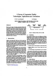
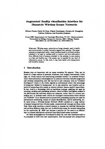
Figure 1: Hard and soft shadows computed in real-time (> 70 FPS), from real-world illumination, using our light factorization.

from the real-world and using this to shade virtual objects. More advanced lighting capture techniques exist, combining knowledge of the surrounding geometry with more detailing directional capture (e.g., from omni-directional cameras) [8], however we build on the simplicity and efficiency of Debevec and Malik’s approach [2]. In augmented reality, work on shading virtual objects can be roughly divided into three groups: traditional computer graphics models, discretized lighting models, and basis-space relighting. The first set of work simply applies simple point/directional lighting models to compute shading (and possibly shadows) from virtual object onto the real scene. With such simple models, the shading of real and virtual objects is inconsistent, causing an unacceptable perceptual gap. Discretized lighting models use more advanced radiosity and instant-radiosity based approaches [6] to compute realistic shading on the virtual objects (at a higher performance cost); however, integrating these techniques in a manner that is consistent with the shading of the real-world objects is an open problem. Thus, the increased realism of the virtual object shading is still overshadowed by the discrepancy between virtual and real shading. Basis-space relighting approaches capture lighting from the real-world and use it to light a virtual object [4]. By construction, the shading on the virtual object will be consistent (to varying degrees) with the real-world shading. However, the coupling of shading between virtual and real objects is a difficult radiometric problem where even slight errors can cause objects to appear to “float” or stand-out from the real-world objects. We address a core component of this problem, computing consistent shading/shadowing on virtual objects and onto perceptually important regions of the realworld. Furthermore, we support animated objects, whereas prior basis-space approaches only handle static geometry. 3 M ATHEMATICAL OVERVIEW AND N OTATION We adopt the following notation: italics for scalars and 3D points/vectors (e.g., ω), boldface for vectors and vector-valued functions (e.g., y), and sans serif for matrices/tensors (e.g., M). 3.1 Spherical Harmonics Many light transport signals, such as the incident radiance at a point, are naturally expressed as spherical functions. The spherical harmonic (SH) basis is the spherical analogue of the Fourier basis and can be used to compactly represent such functions. We summarize some key SH properties (that we will exploit during shading) below, and leave rendering-specific properties to Section 6.

Definition. The SH basis functions are defined as follows:  √ −m  √2 Pl (cos θ ) sin(−mφ ), m < 0 m ym 2 Plm (cos θ ) cos(mφ ), m>0 , l (ω) = Kl  0 Pl (cos θ ), m=0

(1)

where ω = (θ , φ ) = (x, y, z) are directions on the sphere S2 , Plm are associated Legendre polynomials, Klm is a normalization constant, l is a band index, and −l ≤ m ≤ l indexes basis functions in band-l. Basis functions in band-l are degree l polynomials in (x, y, z). SH R m0 is an orthonormal basis, satisfying S2 ym l (ω) yl 0 (ω)dω = δlm,l 0 m0 , where the Kroenecker delta δx,y is 1 if x = y. Projections and Reconstruction. A spherical function f (ω) can be projected onto the SH basis, yielding a coefficient vector Z

f=

S2

n2

f (ω) y(ω) dω , and: f (ω) ≈ fe(ω) =

∑ fi yi (ω) ,

(2)

i=0

where y is a vector of SH basis functions, the order n of the SH expansion denotes a reconstruction up to band l = n − 1 with n2 basis coefficients, and we use a single indexing scheme for the basis coefficients/functions where i = l(l + 1) + m. Zonal Harmonics. The m = 0 subset of SH, called the zonal harmonics (ZH), exhibit circular symmetry about the z-axis and can be efficiently rotated to align along an arbitrary axis ωa . Given an order-n ZH coefficient vector, z, with only n elements (at the m = 0 projection coefficients), we can compute the SH coefficients corresponding to this function rotated from z to ωa as in [12] p gm 4π/(2l + 1) zl ym (3) l = l (ωa ) . In Section 6, we exploit this fast rotation expression for efficient rendering with a variety of different surface BRDF models. SH Products. Given functions f and g, with SH coefficient vectors f and g, the SH projection of the product h = f × g is " #" # Z Z hi =

S2

h(ω) yi (ω) dω ≈

S2

∑ f j y j (ω) ∑ gk yk (ω) j

yi (ω) dω

k

Z

= ∑ f j gk jk

S2

y j (ω) yk (ω) yi (ω) dω = ∑ f j gk Γi jk ,

(4)

jk

where Γ is the SH triple-product tensor. Computing these general products is expensive, despite Γ’s sparsity, but by keeping one of the functions constant, a specialized product matrix can be used: h i Mf = ∑ fk Γi jk such that h = Mf · g. (5) ij

k

In Section 6, we will use specialized product matrices for shading. 3.2 Placement and Geometric Calibration An essential component of any reliable AR system is the computation of a consistent coordinate frame relative to the camera. Two common approaches are marker-based and markerless tracking. Marker-based approaches compute a coordinate frame that remains consistent and stable under significant camera/scene motion. Markerless based tracking instead relies on computer vision algorithms to establish this coordinate frame, but these techniques cannot provide scale information and can become unstable during camera/scene motion. The strength of markerless tracking lies in its generality: no markers are required whereas, for marker-based tracing, if a marker is occluded, unexpected results may be computed. Our work focusses on consistent lighting and shading given a pre-calibrated AR coordinate frame, and so we build on previous

techniques and combine marker-based and markerless approaches to obtain robust correspondence, even under camera/scene motion. We place a marker on the planar surface we wish to place our virtual objects on, detect the position and orientation of the marker using the ARToolKitPlus library [13], and find a mapping between this coordinate frame and the coordinate frame computed with the PTAM markerless tracking library [5]. To do so, PTAM computes a homography from corresponding feature points of the two captured images. The dominant plane of the feature points is placed at the z = 0 plane, forming our initial coordinate frame. The ARToolKitPlus has a coordinate system centered on the marker (see inset) and, given the two images, can compute the positions (p1 , p2 ) and rotations (R1 , R2 ) relative to the marker. PTAM can similarly compute positions ( pˆ1 , pˆ2 ) and rotab1, R b 2 ) with respect to its coordinate frame. tions (R b1, R b 2 ) specify the In a global coordinate frame (R1 , R2 ) and (R same set of rotations, and so the rotation that maps from ARToolKb −1 · R1 = R b −1 · R2 . itPlus’ frame to PTAM’s frame is R = R 1 2 All that remains is to determine the relative scale and translation between the two frames. First we compute the intersection point o of two rays with origins ( pˆ1 , pˆ2 ) and directions (dˆ1 , dˆ2 ) = (R · (−p1 ), R · (−p2 )). These rays are not only guaranteed to intersect, but will do so at the origin of the marker (relative to the PTAM frame). The parametric intersection distance and relative scale are   (dˆ1 )x ( pˆ2 )y − ( pˆ1 )y − (dˆ1 )y [( pˆ2 )x − ( pˆ1 )x ] t kdˆ2 k and s = . t= kp2 k (dˆ1 )y (dˆ2 )x − (dˆ1 )x (dˆ2 )y 4 R EAL -W ORLD L IGHTING In order to shade virtual characters, and static geometry, in a manner that is consistent with the real-world, it is important to capture and apply the lighting from the surrounding environment to these virtual elements. We combine the two most common virtual lighting models in mixed reality, traditional point/directional lights and environmental light probes, in a novel manner. Point and directional lights are a convenient for lighting virtual objects, supporting many surface shading (BRDF) and shadowing models. However, these lights rarely match lighting distributions present in real-world scenes, even with many such lights as in e.g. instant radiosity based approaches [6]. Moreover, the hard shadows that result from using these approaches can appear unrealistic, especially when viewed next to the soft shadows of real objects. On the other hand, environmental light probes can be used to shade virtual objects with lighting from the real scene, increasing the likelihood of consistent appearance between real and virtual objects (see Figure 2). One drawback is that, while shadow functions can be precomputed for static virtual objects, it is difficult to efficiently compute soft shadows (from the environmental light) from virtual objects onto the real world and animated virtual objects. We first discuss two techniques for capturing real-world lighting (Section 4.1), followed by a factorization of the this lighting (Section 5) that allows us to both shade and shadow virtual objects in a manner that is consistent with the real scene (Section 6). 4.1 Capturing Environmental Lighting In Section 6 we show how to compute the shade at a point x in the direction towards the eye ωo , Lout (x, ωo ). This requires (among other things) the incident lighting distribution at x, Lin (x, ω). In our work, we assume that the spatial variation of lighting in the scene can be aggregated into the directional distribution, represented as an environment map of incident light, so that Lin (x, ω) = Lenv (ω). We now outline the two approaches we use to capture Lenv . Mirror Ball Capture. We place a mirror sphere at a known position relative to a marker and use the ARToolkitPlus marker-based feature tracking library [13] to detect the camera position relative

Dominant Light Direction. Starting with the simpler case of monochromatic incident light L(ω) (with SH coefficients L), the linear (l = 1) SH coefficients are scaled linear monomials in y, z and x respectively, and thus encode the 1st -moment vector direction (ignoring coordinate permutations and scale factors) of the spherical function they represent (in this case, the monochromatic light): d~ =

Z  S2

ωx , ωy , ωz

T

· L(ω) dω ,

(8)

where (ωx , ωy , ωz ) are the Cartesian coordinates of ω. In this case, d~ is the principal light vector and, from Equations 1 and 8, we can solve for the normalized principal light direction in terms of L as " (−L3 , −L1 , L2 ) =

#− 1

3

2

2

(−L3 , −L1 , L2 ) ,

∑ (Li )

(9)

i=1

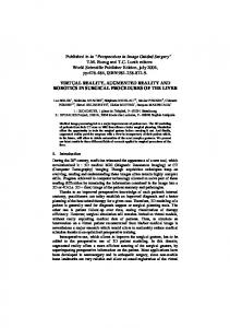
Figure 2: Our light factorization allows for consistent lighting between virtual and real objects: note the consistent shading, from environmental light bounces, and shadows from captured light sources.

to the sphere. We require a parameterization of the sphere image we capture in order to project it into SH (see below). If we normalize the image coordinates of the (cropped) sphere image to (u, v) = [−1, 1] × [−1, 1], we√can map spherical coordinates as ωuv = (θ , φ ) = (arctan(v/u), π u2 + v2 ). Furthermore, when discretizing Equation 2, we compute f ≈ ∑ f (ωuv ) y(ωuv ) dωuv ,

(6)

u,v

where dωuv = (2π/w)2 sinc(θ ) uses the width w in pixels of the (square) cropped mirror sphere image [2]. Free Roaming Capture. In the case where using a markerbased system is not feasible, we can capture an approximation of the environment lighting using the PTAM library [5]. We capture images of the surrounding environment and, for each image, place a virtual omnidirectional camera at the mean distance of all feature points computed by PTAM for that image. The image is then projected to the 6 faces of a virtual cube (placed in a canonical orientation upon system initialization). We similarly require a discrete projected solid angle measure when computing Equation 6 using this cube map parameterization. With the normalizaed image coordinates (u, v) on a cube’s face and the width w in pixels for a side of the cube, we have (as in [9]) h i t = 1 + u2 + v2 and dωuv = 4 t −(3/2) /w2 .

(7)

where we use SH single indexing here for compactness. While we could use more complex approaches (e.g., [9]) for the trichromatic lighting case, we instead choose a simpler, more efficient technique: we convert trichromatic lighting coefficients into monochromatic coefficients using the standard color-to-grayscale conversion. Thus, the dominant light direction can be extracted from Lenv as 

[r]

−L3  ωd =  −L[r] 1 [r] L2

[g]

−L3 [g] −L1 [g] L2

   [b] −L3 0.3 [b]   0.59  . −L1  · [b] 0.11 L2

Dominant Light Color. Given the dominant lighting direction ωd , we now determine the dominant light color in this direction. To determine this color, we place a planar reflector perpendicular to a unit intensity SH directional light at ωd , and compute its albedo so that it reflects unit radiance. Given a planar diffuse reflector with a normal ωd , the SH coefficients of a directional light at ωd that yields unit outgoing radiance on the plane are αym l (ωd ), where α = 16π/17 for order-3 and order-4 SH, and 32π/31 for order-5 and order-6 SH1 [9]. Similar scaling factors can be derived for non-diffuse reflectance, but we have found that using this factor yields plausible results, regardless of the underlying surface BRDF used at run-time (see Section 6). We can now analytically solve for the color as " # " # c[·] =

1

∑

m=−1

[·]

α ym 1 (ωd ) L2+m /

1

∑

2 (α ym . 1 (ωd ))

5

L IGHTING FACTORIZATION

We propose a two-term factorization of the environmental lighting into a directional term Ld (ω) and a residual global lighting Lg (ω), and we will enforce that Lenv (ω) = Ld (ω) + Lg (ω). Given the SH projection coefficients for each color channel of Lenv , {L[r] , L[g] , L[b] }, our factorization seeks to compute a dominant light direction/color, treat it as a separate incident lighting signal, and leave a residual lighting signal which corresponds to nondominant lighting (e.g., from broad area light sources and smooth indirect light bouncing off of surrounding surfaces).

(11)

m=−1

Final Factorization. Given ωd and RGB color (c[r] , c[g] , c[b] ), the directional term of our factorization and its SH projection are [·]

In Section 7 we discuss how we implement high-performance capture and discretized SH projection completely on the GPU.

(10)

Ld (ω) = c[·] δ (ωd ) and Ld = α c[·] ym l (ωd ) .

(12)

The global term and its SH projection are [·]

[·]

Lg (ω) = Lenv (ω) − Ld (ω) and Lg = L[·] − Ld .

(13)

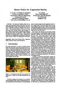
Note that the factorization is “perfect”, in the sense that the environmental light can be perfectly reconstructed from the directional and global terms (both in the primal and SH spaces; see Figure 3). In Section 6, we use this factorization to combine several shading/shadowing models, resulting in realistic shading with hard and soft shadows that is consistent with shading on real-world objects. 1 The α values are shared across two orders because the SH projection of the clamped cosine kernel vanishes for all even bands above l = 2.

Lighting Lenv (ω)

SH projection eenv (ω) L

Directional Ld (ω)

Model f + (x, ωo , ω) ZH coefficients zl Lambertian (nx · ω) h [0.282, 0.326, 0.158, 0] i 0.282(s+2) 0.631s(s+2) 0.746(s−1) Phong (ωr · ω)s , , 0.489, 2 s+1 (s+4) s +4s+3 Mirror δ (ω = ωr ) [0.282, 0.489, 0.631, 0.746]

Global Lg (ω)

ωr is the reflection of ωo about nx and s is the Phong exponent. Table 1: Analytic form of the BRDFs we use and their ZH coefficients.

Synthetic Test Data

Captured Data Figure 3: Factorization into directional and global lighting terms.

6 S HADING WITH FACTORIZED R EAL -W ORLD L IGHTING Direct lighting at a point x towards the eye from the environment is S2

Lenv (ω) V (x, ω) f + (x, ωo , ω) dω

(14)

where V (x, ω) is the binary visibility function that is 1 for directions that are not occluded by geometry, and 0 otherwise, and f + (x, ωo , ω) = f (x, ωo , ω) (nx · ω) is a combination of the viewevaluated BRDF f (x, ωo , ω) and a cosine foreshortening term. There are several challenges to accurately solving Equation 14. Firstly, we must integrate over all lighting directions. Secondly, during integration, we need to evaluate the binary visibility function which, in the most general case, requires tracing rays through the scene for each lighting direction (and at each x). Previous work has either approximated Lenv (or, more generally, Lin ) with many point lights, or assumed static geometry where V can be precomputed and stored at a discrete set of x’s. In the first case, a point light approximation allows for visibility to be computed using e.g. shadow maps, however many such point lights may be required and the cost of computing and shading with many shadow maps quickly becomes the bottleneck of these approaches. In the latter case, if static scene geometry is assumed, SH based shading approaches (which we will discuss below) can be used to quickly integrate over the many lighting directions (without explicitly discretizing them into e.g. individual point lights) and, along with precomputed visibility data, can compute soft shadows that respond to the dynamic lighting environment. Unfortunately, these approaches cannot handle animating or deforming geometry, since the visibility changes at run-time in these instances. We instead exploit our factorization, using a combination of approaches to solve the two problems of light integration and dynamic visibility computation. Substituting Equation 13 into 14 yields Z

Lout (x, ωo ) =

S2

Ld (ω) V (x, ω) f + (x, ωo , ω) dω +

Z

Lg (ω) V (x, ω) f + (x, ωo , ω) S2 g d = Lout (x, ωo ) + Lout (x, ωo )

dω

d Efficient Computation of Lout

d yields Substituting Equation 12 into the definition of Lout d Lout (x, ωo ) =

g

Efficient Computation of Lout

Z S2 [·]

c[·] δ (ωd ) V (x, ω) f + (x, ωo , ω) dω

= c V (x, ωd ) f + (x, ωo , ωd ) .

d in Equation 16, L Unlike Lout out cannot reduce into a single sampling operation since Lg is composed of lighting from all directions. Sampling and evaluating the three terms in the integrand, for all directions at run-time, is not feasible. We exploit the smoothness of Lg and perform this computation efficiently in the SH domain. As discussed earlier, the two main challenges when computing Equation 14 are integration over all light directions and evaluation of the visibility function (at all directions and all x). The expression d also exhibits these problems, below for Lout

(16)

Z

g

Lout (x, ωo ) =

S2

Lg (ω)V (x, ω) f + (x, ωo , ω)dω ,

(17)

and we will first discuss the integration problem (assuming we have a solution to the visibility problem), and then discuss several approaches we employ for solving the visibility problem2 . Integration with SH. As we readily have the SH projection of Lg , Lg (from Section 4.1), suppose we can express V and f + with SH projections V and f, then the most general solution to Equation 17 using SH involves summing over the triple-product tensor, " #" #" # Z   g Lout ≈ ∑ Lg i yi (ω) ∑ V j y j (ω) ∑ fk yk (ω) dω S2

i

j

k

  = ∑ Lg i V j fk Γi jk ,

(18)

i jk

which is a computationally expensive procedure, particularly when executed at every x. Alternatively, in the case where one of the three terms in the integrand is known beforehand, we can precompute the SH product matrix of this function to accelerate the computation. For example, we could precompute a product matrix for Lg as h i h i   g MLg = ∑ Lg k Γi jk such that Lout ≈ ∑ MLg · f Vi . (19) ij

(15)

and we will discuss solutions to each of these terms independently. 6.1

6.2

g

Z

Lout (x, ωo ) =

In this form, integration over light directions is replaced by a single evaluation and visibility can be computed using shadow maps. The BRDF models we use when evaluating f + (as well as their ZH representations; see Section 6.2) are summarized in Table 1. Although Equation 16 requires a simple application of shadowed point lighting, the parameters of this model are carefully derived in our factorization to maintain consistency with the global shading term, which we evaluate without explicitly sampling any lighting d and Lg , and the directions (Section 6.2). The combination of Lout out manner in which Ld and Lg are derived and applied, which makes the use of point lighting acceptable for our solution.

k

i

i

Equation 19 avoids the per-point evaluation of the triple-product tensor in Equation 18, offloading this computation to a one-time (per lighting update) evaluation of the triple-product when computing MLg ; the run-time now involves a simpler matrix-vector product following by a dot-product. Note that we construct the product matrix for the lighting, instead of the BRDF, since lighting will change at most once per-frame whereas the view-evaluated 2 We

drop the [·] superscript for color channel indexing, and assume that all equations are applied to each color channel independently.

BRDF(s) changes at least once per frame (and potentially once per point if we do not assume a distant viewer model). We can further simplify run-time evaluation if two of the three integrand terms are known apriori. For example, in the case of static geometry and diffuse reflection, the product T (x, ω) = V (x, ω) × f + (x, ω) can be projected into SH during precomputation, yielding the following run-time computation3 Z

[Tx ]i =

S2

  g T (x, ω)yi (ω)dω such that Lout ≈ ∑ [Tx ]i Lg i , (20) i

which corresponds to the standard PRT double product [11] and can be easily derived using the orthonormality property of SH. One detail we have not discussed is how to compute the SH projection of the view-evaluated BRDF. We currently support the three common BRDF models in Table 1. Each of these BRDFs are circularly symmetric about an axis: the Lambertian clamped cosine is symmetric about the normal nx , and the Phong and Mirror BRDFs are symmetric about the reflection vector ωr . At run-time, the SH coefficients of the BRDFs is computed using Equation 3 and the order-4 ZH coefficients listed in Table 1. We note that, in the case of perfect mirror reflection, instead of inducing a blur on the (very sharp) mirror reflection “lobe”, we exploit the fact that we have captured Lenv (ω) and can readily sample Lg (ω). In this case, we sample the SH-projected visibility when reconstructing the global lighting shade as g

Lout ≈ Lg (ωr )

∑ Vi yi (ωr ) .

(21)

i

Figure 4 illustrates the different BRDF components for an object shaded with only the global lighting.

Diffuse

Glossy

Mirror

Figure 4: Shading, including soft shadows, from global/ambient light (directional light omitted) due to each BRDF component (> 70 FPS).

While we have discussed shadowing for directional lighting, we have so far assumed that the SH projection of binary visibility at x, V, was readily available for use in shadowing the global lighting. Below we discuss the different ways we compute V. SH Visibility. We discuss different shadowing models for global lighting, depending on the type of virtual object we are shading. For static objects, we use either standard PRT (Equation 20) for diffuse objects or precomputed SH visibility product matrices and Equation 19 (replacing MLg with a product matrix for visibility). For animating or deformable objects, we segment shadowing into two components: cast shadows from the object onto the environment, and self shadows from the object onto itself. For cast shadows, we are motivated by previous work on spherical blocker approximations [7]. We fit a small number (10 to 20) of spheres to our animating geometry (e.g., in its rest pose for articulated characters) and skin their positions during animation. Shadowing is due to the spherical proxy geometry, as opposed to the actual underlying geometry. The use of spherical blocker approximation is justified in two ways. Firstly, since the global lighting component is a smooth spherical function, equivalent to large and broad area light sources, fine scale geometry details will be lost in 3 Note

that f + (x, ωo , ω) = f + (x, ω) in the case of diffuse reflectance.

the smooth shadows that are produced by these types of area lights. Secondly, SH visibility can be efficiently computed using sphere blockers, as we will now discuss. Considering only a single sphere blocker, the visibility function due to that blocker is a circularly symmetric function, and so if we align the vector from x to the center of the blocker with the z axis, the single sphere visibility is defined as in [7],  0, if arccos (ω · z) ≤ arcsin ( dr ) Vs (ω) = (22) 1, otherwise , and has ZH coefficients Z

Vs = "

S2

Vs (ω) y(ω)dω

  √ √ 0.6R −4d 2 + 5r = 1.8 1 + 1 − R , −1.5R, −2R 1 − R, d2

(23)
# 2 ,

where R = (r/d)2 . If we approximate our animated object with a single sphere, applying Equation 3 to Equation 23 will yield V, which can be used in Equation 19 to compute the final shade. However, it is rarely the case that a single blocker sphere is sufficient. In the case of multiple spheres, SH products of the visibility from individual spheres must be taken to compute the total visibility V. Instead of computing SH visibility for a sphere at a time and applying Equation 4 (which requires expensive summation of Γ, for each sphere), we compute an analytic product matrix for a single sphere blocker oriented about an arbitrary axis by combining Equations 23, 3 and 5. In the case of only a few blocker spheres (e.g., if we only model cast shadows from the feet of a character onto the ground, using two spheres), applying the precomputed sphere blocking product matrix to Lg (or f) and shading with Equation 19 is an efficient solution. However, as we increase the number of spherical blockers (and thus, the number of product matrix multiplications), performance degrades rapidly. In this case, we accelerate this SH multi-product by performing computation in the logarithmic SH domain [7]. The technique of Ren et al. [7] computes the SH projection of log (Vs (ω)) (which, in the canonical orientation, is still a ZH) and tabulates these coefficients as a function of (r/d). Rotated log SH coefficients are computed for each sphere blocker, using Equation 3, and summed together yielding a net log SH visibility vector, Vlog . We use the tabulated values provided by Ren et al. [7] and directly apply the “optimal linear” SH exponentiation operator to convert the net log SH visibility to the final SH visibility vector as    √   b log k 1 + b kV b log k V b log , (24) a kV V ≈ exp Vlog 0 / 4π √ b log is Vlog with its DC term set to 0, and 1 = ( 4π, 0, . . . , 0) where V is the SH projection of the constant function one(ω) = 1. For self-shadows, Ren et al. [7] propose “sphere replacement rules” for handling shade points that lie on the surface of the mesh (potentially within the volume of several blocker spheres), however we use a simpler solution that yields suitable results. We precompute and store the DC projection of visibility, which is related to ambient occlusion, at vertices of the dynamic object. At run-time, we need only scale the unshadowed lighting by this occlusion factor. This is equivalent to using Equation 19 with only V0 6= 0; in the case of triple product integration, if one of the terms has only a non-zero DC component, this is equivalent to scaling the double product integration by the DC component of the third (DC-only) term in integrand [9]. Unshadowed light is computed by rotating the appropriate ZH vector from Table 1 using Equation 3, and then computing the double product integral (as in Equation 20) of Lg with these rotated BRDF coefficients. Figure 5 illustrates the contribution of the different shadowing components we use.

Unshadowed

Cast Shadows

Self-Shadows

set of directional and environment lights), or by using looping constructs in a rendering single-pass. All of our results run at higher than 70 FPS, including all geometric calibration, lighting and shading computations. We did not focus much effort on optimizing our implementation: we use standard implementations of shadow mapping with PCF, and we perform all SH shading using straightforward implementation of the equations included in the exposition. We interface directly with PTAM and ARToolKitPlus implementations provided online. 8

Direct Shadow

Sphere Proxies (with both shadows)

Final Image

Figure 5: Top row: smooth cast shadows (middle) and self-shadows (right) due to global lighting give subtle depth and lighting cues compared to no shadows (left). Bottom row: directional shadows (left), visualizing blocker spheres with directional and cast shadows (middle), and the final composited image (right; rendered at > 70 FPS).

7

I MPLEMENTATION

AND

P ERFORMANCE

We benchmark our system on an Intel Core2 Duo 2.8 GHz Laptop with an NVidia Quadro FX 770M GPU. We use the PlayStation Eye camera for capture. Our end-to-end algorithm performs the following computations, implementing the equations directly in GLSL: – – – –

At initialization, compute geometric calibration (Section 3.2), Capture lighting from mirror sphere or free roaming (Section 4), Compute SH projection of Lenv (see details below; Equation 6), Compute Ld and Lg using lighting factorization (Section 5),

d (see details below; Section 6.1 and Equation 16), – Compute Lout g

– Compute Lout (Section 6.2), and – Composite direct and global shading components. We compute the SH projection of the captured lighting by precomputing y(ωuv ) dωuv values in a texture and use graphics hardware to quickly multiply this precomputed texture with the captured lighting image, Lenv (ωuv ). Depending on the spherical parameterization (sphere vs. cube), we use the appropriate definition of dωuv as well as the appropriate texture image layout (i.e., six textures are required for the cube map case). The summation in Equation 6 is computed with a multi-pass sum on the GPU, manually implementing a mip-map reduction where each pass averages 4 × 4 pixel blocks and results in an output texture of half the size (per dimension). Table 2 summarizes the light projection performance. Mirror Sphere Capture and Projection Find Markers LDR to HDR SH Project Total 4 ms 0.6 ms 1.7 ms 6.3 ms Free Roaming Capture and Projection Find Homography LDR to HDR Map to Cube SH Project Total 2 ms 0.8 ms 1.1 ms 1.8 ms 5.7 ms Table 2: Performance breakdown for capturing and projecting realworld illumination into SH using our two capture methods. d with Equation 16, we use a 1024 × 1024 When computing Lout 24-bit shadow map, and 4 × 4 percentage-closer filtering [3]. All shading computations are performed on the GPU using GLSL shaders with lighting coefficients computed every frame, which allows for dynamic lighting response. We usually use a single directional light and environment light, however the performance of our approach degrades linearly with additional lights. In this manner, we can support an arbitrary number of directional and environment lights using either multi-pass deferred rendering (one pass for each

D ISCUSSION

In all cases, we factor out a single directional light from the captured environment. Since factorization takes place in the SH domain, the extracted directional lighting information is robust to high-frequency noise or motion artifacts in the raw captured lighting signal. Such high-frequency issues may only affect the quality of mirror reflections, where the captured lighting is used without filtering, but no such artifacts arose in our examples. Previous work in AR relighting has used subsets of the techniques we implement, without lighting factorization, however an alternative approach based on instant radiosity also targets similar smooth and sharp shading effects in AR applications [6]. Our approach shares the following similarities to this previous work: both compute lighting from the real environment prior to compositing the shading from virtual objects, and both make similar assumptions about the BRDFs of the real world objects (neither technique properly handles specularities from real objects). While more general (i.e., color bleeding from virtual objects can be approximated), this instant radiosity based approach requires higher end hardware and still achieves lower performance. In the case of static geometry, we could integrate real objects into the PRT preprocess, but this would incur similar performance penalties as the instant radiosity procedure. Our approach combines lighting factorization with several different rendering approaches, each targeting a specific shading component, in order to achieve a final consistent (albeit approximate) shading result. The instant radiosity approach instead applies a single rendering algorithm that models many different lighting paths. Both approaches have their merits, and we opted for a lighter weight solution based on a novel lighting factorization. Exploiting the inherent smoothness of SH projection also allows us to reduce temporal artifacts that are commonly present in instant radiosity approaches. The quality of our results are suitable for interactive applications (e.g. gaming), where response rate is more important than physical accuracy. We are able to handle dynamic changes in the lighting and camera (see our video), maintaining consistent shading between real and virtual objects. In a few scenarios, the extracted dominant lighting direction exhibits low-frequency noise during animation; we are investigating windowing and filtering approaches to maintain a more robust temporal estimate of the dominant lighting direction. Limitations. Our factorization currently only supports extraction of a single directional light. While this can perform well in many indoor (e.g. room with a dominant light source) and outdoor (e.g. forest environment on a sunny day) scenarios, many realworld lighting situations have several dominant light sources. In these cases, our approaches folds all “secondary” dominant lights into the global lighting term; combining ideas from Sloan’s multilight extraction approach [9] with our rendering algorithm is one approach to solve this problem, however handling temporal flickering issues may become a larger problem in these cases. Moreover, as mentioned earlier, we do not support bounced light from virtual objects onto real objects. An approximate solution based on the sphere proxies [10] can be implemented, however a more accurate proxy of the real-world geometry is necessary. Lastly, we have only applied rudimentary tone mapping to our input

images, and developing a more complete, interactive high-dynamic range capture and rendering solution is left to future work. 9

C ONCLUSIONS

AND

F UTURE W ORK

We presented a technique to factor environmental light emitting from, and bouncing off, the real-world. Our factorization is designed to directly support both hard and soft shadowing techniques. Using basis-space relighting techniques and GPU acceleration, we can efficiently compute shadows from both static and animated virtual objects. The manner in which we factor and combine different illumination contributions is novel, and generates more consistent shading than previously possible (e.g., with only the individual application of any one of the techniques we incorporate). Traditional cast shadows in AR are sharp and colored in a manner that does not respond to the surrounding lighting, whereas our hard shadows are shaded based on dynamic environmental ambient light. Moreover, soft shadows due to residual global lighting add physically-based smooth shading, increasing perceptual consistency in a manner similar to diffuse interreflection. Our factorization roughly identifies a direct lighting and “intelligent” bounced lighting terms, however we still apply directillumination integration to these components, ignoring the effects of indirect light bounces from the virtual objects onto the real-world geometry. In the future we plan on incorporating such effects by, for example, modeling light bouncing off of the sphere proxies [10]. ACKNOWLEDGEMENTS We thank Paul Debevec for the light probes, and Zhong Ren for the humanoid mesh and tabulated log SH sphere blocker data. R EFERENCES [1] P. Debevec. Rendering synthetic objects into real scenes: bridging traditional and image-based graphics with global illumination and high dynamic range photography. In SIGGRAPH, NY, USA, 1998. ACM. [2] P. E. Debevec and J. Malik. Recovering high dynamic range radiance maps from photographs. In SIGGRAPH, NY, USA, 1997. ACM Press/Addison-Wesley Publishing Co. [3] R. Fernando. Percentage-closer soft shadows. In SIGGRAPH Sketches, NY, USA, 2005. ACM. [4] S. Heymann, A. Smolic, K. M¨uller, and B. Froehlich. Illumination reconstruction from real-time video for interactive augmented reality. International Workshop on Image Analysis for Multimedia Interactive Services (WIAMIS ’05), 2005. [5] G. Klein and D. Murray. Parallel tracking and mapping for small AR workspaces. In Proc. 6th IEEE and ACM International Symposium on Mixed and Augmented Reality (ISMAR’07), Nara, Japan, Nov 2007. [6] M. Knecht, C. Traxler, O. Mattausch, W. Purgathofer, and M. Wimmer. Differential instant radiosity for mixed reality. ISMAR ’10: Proceedings of the 2010 9th IEEE International Symposium on Mixed and Augmented Reality, Oct. 2010. [7] Z. Ren, R. Wang, J. Snyder, K. Zhou, X. Liu, B. Sun, P.-P. Sloan, H. Bao, Q. Peng, and B. Guo. Real-time soft shadows in dynamic scenes using spherical harmonic exponentiation. In SIGGRAPH, NY, USA, 2006. ACM. [8] I. Sato, Y. Sato, and K. Ikeuchi. Acquiring a radiance distribution to superimpose virtual objects onto a real scene. IEEE Transactions on Visualization and Computer Graphics, 1999. [9] P.-P. Sloan. Stupid spherical harmonics (SH) tricks. Game Developers Conference, 2009. [10] P.-P. Sloan, N. K. Govindaraju, D. Nowrouzezahrai, and J. Snyder. Image-based proxy accumulation for real-time soft global illumination. In Pacific Graphics, USA, 2007. IEEE Computer Society. [11] P.-P. Sloan, J. Kautz, and J. Snyder. Precomputed radiance transfer for real-time rendering in dynamic, low-frequency lighting environments. In SIGGRAPH, NY, USA, 2002. ACM. [12] P.-P. Sloan, B. Luna, and J. Snyder. Local, deformable precomputed radiance transfer. In SIGGRAPH, NY, USA, 2005. ACM.

[13] D. Wagner and D. Schmalstieg. ARToolKitPlus for pose tracking on mobile devices artoolkit. Proceedings of 12th Computer Vision Winter Workshop (CVWW ’07), 2007.