AbstractâThis paper describes the synthesis method of linear array geometry with minimum sidelobe level and null control using the particle swarm optimization ...
2674
IEEE TRANSACTIONS ON ANTENNAS AND PROPAGATION, VOL. 53, NO. 8, AUGUST 2005
Linear Array Geometry Synthesis With Minimum Sidelobe Level and Null Control Using Particle Swarm Optimization Majid M. Khodier, Member, IEEE, and Christos G. Christodoulou, Fellow, IEEE
Abstract—This paper describes the synthesis method of linear array geometry with minimum sidelobe level and null control using the particle swarm optimization (PSO) algorithm. The PSO algorithm is a newly discovered, high-performance evolutionary algorithm capable of solving general -dimensional, linear and nonlinear optimization problems. Compared to other evolutionary methods such as genetic algorithms and simulated annealing, the PSO algorithm is much easier to understand and implement and requires the least of mathematical preprocessing. The array geometry synthesis is first formulated as an optimization problem with the goal of sidelobe level (SLL) suppression and/or null placement in certain directions, and then solved by the PSO algorithm for the optimum element locations. Three design examples are presented that illustrate the use of the PSO algorithm, and the optimization goal in each example is easily achieved. The results of the PSO algorithm are validated by comparing with results obtained using the quadratic programming method (QPM). Index Terms—Antenna array, null control, particle swarm optimization (PSO), sidelobe suppression.
I. INTRODUCTION
T
HE goal in antenna array geometry synthesis is to determine the physical layout of the array that produces the radiation pattern that is closest to the desired pattern. The shape of the desired pattern can vary widely depending on the application. Many synthesis methods are concerned with suppressing the sidelobe level (SLL) while preserving the gain of the main beam. Other methods deal with the null control to reduce the effects of interference and jamming. For the linear array geometry, this can be done by designing the spacings between the elements, while keeping a uniform excitation over the array aperture. Other methods of controlling the array pattern employ nonuniform excitation and phased arrays [1]. Evolutionary algorithms such as genetic algorithms (GA) [2]–[8], simulated annealing (SA) [9], and particle swarm optimization (PSO) algorithms [10], [11] have also been successfully used in the design of antenna arrays. The PSO algorithm has been shown to be an effective alternative to other evolutionary algorithms in handling certain kinds of optimization problems. Compared to GA and SA, the PSO algorithm is much easier to implement and apply to design problems with continuous or discontinuous parameters. Manuscript received September 8, 2004; revised December 15, 2004. M. M. Khodier is with the Department of Electrical Engineering, Jordan University of Science and Technology, Irbid 22110, Jordan (e-mail: majidkh@ just.edu.jo). C. G. Christodoulou is with the Department of Electrical and Computer Engineering, The University of New Mexico, Albuquerque, NM 87131 USA. Digital Object Identifier 10.1109/TAP.2005.851762
N
Fig. 1. Geometry of the 2 -element symmetric linear array placed along the x-axis.
The PSO has been recently used to design the excitation distribution of linear arrays [6], [7], and to optimize the profile of a corrugated horn antenna [12]. In this paper, the PSO is used to optimize the spacings between the elements of the linear array to produce a radiation pattern with minimum SLL and null placement control. The array geometry is shown in Fig. 1. We assume isotropic radiators placed symmetrically along that we have the x-axis. Due to the symmetry, the array factor in the azimuth plane (x-y plane) can be written as (1) , and are, respecwhere is the wavenumber, and , tively, the excitation amplitude, phase, and location of the th element. If we further assume a uniform excitation of amplitude and for all elements), the array and phase (that is factor can be written as (2) Now the statement of the current problem simply reduces to: use the PSO algorithm to find the locations, , of the array elements that will result in an array beam with minimum SLL and, if desired, nulls at specific directions. II. PSO The PSO algorithm is an evolutionary algorithm capable of solving difficult multidimensional optimization problems in various fields. Since its introduction in 1995 by Kennedy and Eberhart [13], the PSO has gained an increasing popularity as
0018-926X/$20.00 © 2005 IEEE
KHODIER AND CHRISTODOULOU: LINEAR ARRAY GEOMETRY SYNTHESIS
2675
TABLE I GEOMETRY OF THE 10-ELEMENT LINEAR ARRAY OBTAINED USING THREE DIFFERENT METHODS. THE NUMBERS ARE NORMALIZED WITH RESPECT TO �=2
Fig. 2.
Flowchart showing the main steps of the PSO algorithm.
an efficient alternative to GA and SA in solving optimization design problems in antenna arrays. As an evolutionary algorithm, the PSO algorithm depends on the social interaction between independent agents, here called particles, during their search for the optimum solution using the concept of fitness. It should be mentioned here that this paper is not intended to be an extensive review of the PSO algorithm, and therefore only the main steps of the algorithm are reviewed here. The reader is referred to [10]–[18] and the references mentioned therein for a detailed discussion of the basic concepts of the PSO algorithm and how it works. The main steps of the PSO algorithm are shown in Fig. 2 in a flowchart diagram. After defining the solution space and the fitness function, the PSO algorithm starts by randomly initializing the position and velocity of each particle in the swarm. For an -dimensional problem, the position and velocity can be specified by an matrices as follows:
Fig. 3. Normalized patterns of the 10-element linear array obtained using three different methods. The regions of suppressed SLL are [0 , 82 ] and [98 , 180 ], and no prescribed nulls. Array geometry is given in Table I.
the position at which each particle attained its best fitness value up to the present iteration. The personal best positions can be defined by the matrix
..
.
(5)
The global best position vector defines the position in the solution space at which the best fitness value was achieved by all particles, and is defined by (6)
..
.
..
.
(3)
(4)
where is the number of particles in the swarm. Each row of the position matrix represents a possible solution to the optimization problem. The velocity of each particle depends on the distance of the current position to the positions that resulted in good fitness values. To update the velocity matrix at each iteration, every particle should know its personal best and the global best position vectors. The personal best position vector defines
All the information needed by the PSO algorithm is contained in , , , and . The core of the PSO algorithm is the method by which these matrices are updated in every iteration of the algorithm. These matrices are updated such that each particle takes the path of a damped oscillatory movement toward its personal best and the global best positions in every new iteration. To achieve this, the velocity matrix is updated according to [13], [14] (7) refer to the time index of where the superscripts and and are two the current and the previous iterations, uniformly distributed random numbers in the interval [0,1] and
2676
IEEE TRANSACTIONS ON ANTENNAS AND PROPAGATION, VOL. 53, NO. 8, AUGUST 2005
Fig. 4. Convergence curve of the fitness value of the 10-element linear array versus the number of iterations. The PSO algorithm is attempting to reach the minimum value of the function in (9).
Fig. 5. Convergence of the position vector of particle #1 versus the number of iterations. After about 400 iterations, the particle’s position vector settles at the values given in Table I.
these random numbers are different for each of the components of the particle’s velocity vector. The parameters and specify the relative weight of the personal best position versus the global best position. Previous work has shown that a value of 2.0 is a good choice for both parameters [14]. The parameter is a number, called the “inertial weight,” in the range [0,1], and it specifies the weight by which the particle’s current velocity depends on its previous velocity and how far the particle is from its personal best and global best positions. Previous work [12] has shown that the PSO algorithm converges faster if is linearly damped with iterations starting at 0.9 and decreasing linearly to 0.4 at the last iteration. Such damping will slow down the velocity of the particles as they get closer to the global best position, and therefore enhancing convergence speed of the PSO
Fig. 6. Convergence of a particle’s velocity versus the number of iterations. It can be seen that after 500 iterations, the particle’s velocity is indistinguishable from zero.
Fig. 7. Normalized patterns of the 28-element array obtained using three different methods. The SLL suppression region is [0 , 180 ], and prescribed nulls at: 55 , 57.5 , 60 , 120 , 122.5 , 125 . Array geometry is given in Table II.
algorithm. The position matrix is updated at each iteration according to (8) The PSO algorithm, like other evolutionary algorithms, uses the concept of fitness to guide the particles during their search for the optimum position vector in the -dimensional space. The fitness defines how well the position vector of each particle satisfies the requirements of the optimization problem. At each iteration of the algorithm, the particle’s position vector that resulted in the best fitness is chosen as the global best position vector, and this information is passed to all other particles to use in adjusting their velocity and position vectors accordingly. In antenna problems, there are many factors that can be used to evaluate the fitness such as directivity, gain, SLL, size, and weight, depending
KHODIER AND CHRISTODOULOU: LINEAR ARRAY GEOMETRY SYNTHESIS
2677
TABLE II GEOMETRY OF THE 28-ELEMENT LINEAR ARRAY OBTAINED USING THREE DIFFERENT METHODS. THE NUMBERS ARE NORMALIZED WITH RESPECT TO �=2
on the application. For the current problem, we are interested in designing the geometry of a linear antenna with minimum average SLL and null control in specific directions. To achieve this goal, the following function is used to evaluate the fitness: (9) where s are the spatial regions in which the SLL is sup, and s are the directions of the nulls. pressed, For array design with suppressed SLL only, the first term on the right-hand side (RHS) of (9) is used to evaluate the fitness; for null control only, the second term on the RHS of (9) is used; and finally designing for suppressed SLL and null control, both terms on the RHS of (9) are used in the fitness evaluation. For the problem at hand, the particle’s position vector that resulted in the minimum value of the fitness function given in (9) is chosen as the global best position vector up to the current iteration. III. DESIGN EXAMPLES The PSO algorithm outlined in the previous section is illustrated by the following design examples. The PSO algorithm was implemented using MATLAB. To speed up the PSO algorithm, instead of randomly initializing the position matrix at at the beginning of each run, we have chosen to initialize the same element locations of the conventional array, which has between neighboring elements. Fia uniform spacing of nally, all the results were obtained by using a swarm population, , of 20 particles, and a number of iterations large enough to guarantee the convergence of the PSO algorithm to the desired solution. The first example illustrates the synthesis of a 10-element array for minimum SLL in the bands [0 , 82 ] and [98 , 180 ] with no prescribed nulls. The array pattern from the PSO algorithm is shown in Fig. 3, along with patterns obtained using the conventional array geometry, and the quadratic programming method (QPM) as explained in [1], [19]–[24]. The basic idea of the QPM is to form a quadratic program with its cost function given by the mean square error between the array pattern and a carefully selected pattern described by a known mathematical function. The quadratic program can be constrained or unconstrained, depending on the optimization problem requirements. It should be mentioned here that all the results of the QPM for the examples presented in this paper are taken directly from [1]. It can be seen from Fig. 3 that the conventional array exhibits relatively high SLL. The QPM offers an improvement of 1.5 to 5 dB, while the PSO algorithm offers an improvement of 3 to 5 dB in terms of SLL suppression. It can also be seen from Fig. 3 that the close-in sidelobes are almost the same for both the QPM and the PSO, but the far sidelobes are better for
Fig. 8. Same as Fig. 7, but now the pattern is obtained using the PSO algorithm, once with the fitness function as given in (9) and is called “Sum,” and then with the fitness function as given in (10) and is called “Product.” The array geometry obtained by the PSO algorithm for both cases is practically the same.
Fig. 9. Normalized patterns of the 32-element linear array obtained using three different methods. The regions of suppressed SLL are [0 , 87 ] and [93 , 180 ], and prescribed nulls at: 81 , 99 . Array geometry is given in Table III.
the PSO. This is achieved in exchange for a larger width in the main beam. However, it can be seen from Fig. 3 that the 3-dB beamwidth has only slightly increased by less than one degree. The array geometry for this example is shown in Table I. It can be seen from the table that the array length obtained using the PSO algorithm is more or less the same as that of the QPM and conventional arrays. This is also observed for the rest of the design examples shown next.
2678
IEEE TRANSACTIONS ON ANTENNAS AND PROPAGATION, VOL. 53, NO. 8, AUGUST 2005
TABLE III GEOMETRY OF THE 32-ELEMENT LINEAR ARRAY OBTAINED USING THREE DIFFERENT METHODS. THE NUMBERS ARE NORMALIZED WITH RESPECT TO �=2
The convergence of the fitness value versus the number of iterations for the 10-element array is shown in Fig. 4. The figure shows that the fitness value starts at a value of about 0.028 and quickly drops to a flat value of about 0.0105 in about 400 iterations. Fig. 5 shows the convergence of the position vector of particle #1, which, after about 400 iterations, settles at the values given in Table I. All other particles in the swarm behave similarly, and their results are not included in the figure for clarity purposes. The same thing can be said about Fig. 6, which shows the convergence of the velocity vector of one of the particles in the swarm. After 500 iterations, the particle’s velocity becomes indistinguishable from zero. The second example discusses the geometry of a 28-element array designed for SLL suppression in the region [0 , 180 ] and prescribed nulls at: 55 , 57.5 , 60 , 120 , 122.5 , 125 . Fig. 7 shows that a broad null as deep as 50 dB is easily achieved, at least in theory. The PSO algorithm and the QPM [1] give very similar array patterns. The corresponding array geometry is given in Table II. Fig. 8 shows the pattern of the same 28-element array designed by the PSO algorithm using two different fitness functions. The “Sum” curve is obtained using the fitness function as given in (9), and the “Product” curve is obtained using the following fitness function
(10)
Both fitness functions resulted in a deep broad null at the prescribed directions. The array geometries for both cases agree with the numbers from the PSO algorithm given in Table II up to the fourth digit. The third and last example shows the design of a 32-element array with SLL suppression in the regions [0 , 87 ] and [93 , 180 ] and nulls at 81 , 99 . The array pattern is shown in Fig. 9. We note that a deep null (lower than 60 dB) is easily imposed just beside the first sidelobe at 81 , 99 , and the first SLL is still kept 5 to 7 dB below that of the conventional array, and most of the other sidelobes are either suppressed or maintained. The corresponding array geometry is shown in Table III. The convergence of the fitness value for this example is shown in Fig. 10. IV. CONCLUSION This paper illustrated the use of the particle swarm optimization method in the synthesis of linear array geometry for the purpose of suppressed sidelobes and null placement in certain directions. The PSO algorithm was successfully used to opti-
Fig. 10. Convergence curve of the fitness value of the optimized 32-element array whose pattern is shown in Fig. 9.
mize the locations of array elements to exhibit an array pattern with either suppressed sidelobes, null placement in certain directions, or both. In each of these cases, the PSO algorithm easily achieved the optimization goal. More control of the array pattern can be achieved by using the PSO algorithm to optimize, not only the location, but also the excitation amplitude and phase of each element in the array, and exploring other array geometries. As an evolutionary algorithm, the PSO method will most likely be an increasingly attractive alternative, in the electromagnetics and antennas community, to other evolutionary algorithms such as genetic algorithms and simulated annealing. Compared to genetic algorithms and simulated annealing, the PSO algorithm is much easier to understand and implement and requires minimum mathematical preprocessing. REFERENCES [1] Handbook of Antennas in Wireless Communications, L. C. Godara, Ed., CRC, Boca Raton, FL, 2002. [2] Y. Rahmat-Samii and E. Michielssen, Eds., Electromagnetic Optimization by Genetic Algorithms. New York: Wiley, 1999. [3] J. Johnson and Y. Rahmat-Samii, “Genetic algorithms and method of moments (GA/MOM) for the design of integrated antennas,” IEEE Trans. Antennas Propag., vol. 47, no. 10, pp. 1606–1614, Oct. 2001. [4] M. Himdi and J. Daniel, “Synthesis of slot coupled loaded patch antennas using a genetic algorithm through various examples,” in IEEE AP-S Dig., vol. 3, 1997, pp. 1700–1703. [5] F. J. Ares-Pena, J. A. Gonzalez, E. Lopez, and S. R. Rengarajan, “Genetic algorithms in the design and optimization of antenna array patterns,” IEEE Trans. Antennas Propagat., vol. 47, no. 3, pp. 506–510, Mar. 1999. [6] K. K. Yan and Y. Lu, “Sidelobe reduction in array-pattern synthesis using genetic algorithm,” IEEE Trans. Antennas Propag., vol. 45, no. 7, pp. 1117–1122, Jul. 1997.
KHODIER AND CHRISTODOULOU: LINEAR ARRAY GEOMETRY SYNTHESIS
[7] A. Tennant, M. M. Dawoud, and A. P. Anderson, “Array pattern nulling by element position perturbations using a genetic algorithm,” Electron. Lett., vol. 30, no. 3, pp. 174–176, Feb. 1994. [8] B. K. Yeo and Y. Lu, “Array failure correction with a genetic algorithm,” IEEE Trans. Antennas Propag., vol. 47, no. 5, pp. 823–828, May 1999. [9] V. Murino, A. Trucco, and C. S. Regazzoni, “Synthesis of equally spaced arrays by simulated annealing,” IEEE Trans. Signal Process., vol. 44, no. 1, pp. 119–122, Jan. 1996. [10] D. Gies and Y. Rahmat-Samii, “Particle swarm optimization for reconfigurable phased-differentiated array design,” Microw. Opt. Tech. Lett., vol. 38, no. 3, pp. 168–175, Aug. 2003. [11] D. W. Boeringer and D. H. Werner, “Particle swarm optimization versus genetic algorithms for phased array synthesis,” IEEE Trans. Antennas Propag., vol. 52, no. 3, pp. 771–779, Mar. 2004. [12] J. Robinson and Y. Rahmat-Samii, “Particle swarm optimization in electromagnetics,” IEEE Trans. Antennas Propag., vol. 52, no. 2, pp. 397–407, Feb. 2004. [13] J. Kennedy and R. C. Eberhart, “Particle swarm optimization,” in Proc. IEEE Conf. Neural Networks IV, Piscataway, NJ, 1995. [14] R. C. Eberhart and Y. Shi, “Particle swarm optimization: developments, applications and resources,” in Proc. 2001 Congr. Evolutionary Computation, vol. 1, 2001. [15] G. Ciuprina, D. Ioan, and I. Munteanu, “Use of intelligent-particle swarm optimization in electromagnetics,” IEEE Trans. Magn., vol. 38, no. 2, pp. 1037–1040, Mar. 2004. [16] J. Park, K. Choi, and D. J. Allstot, “Parasitic-aware RF circuit design and optimization,” IEEE Trans. Circuits Syst.-I, vol. 51, no. 10, pp. 1953–1966, Oct. 2004. [17] I. C. Trelea, “The particle swarm optimization algorithm: convergence analysis and parameter selection,” Inform. Processing Lett., vol. 85, pp. 317–325, 2003. [18] K. E. Parsopoulos and M. N. Vrahatis, “Recent approaches to global optimization problems through particle swarm optimization,” Natural Computing, vol. 1, pp. 235–306, 2002. [19] B. P. Ng, “Designing array patterns with optimum inter-element spacings and optimum weights using a computer-aided approach,” Int. J. Electron., vol. 73, no. 3, 1992. [20] B. P. Ng, M. H. Er, and C. A. Kot, “Linear array aperture synthesis with minimum sidelobe level and null control,” Inst. Elect. Eng. Proc.- Microw. Antennas Propag., vol. 141, no. 3, Jun. 1994. [21] B. P. Ng, “Array synthesis using a simple computer-aided approach,” Inst. Elect. Eng. Electron. Lett., vol. 26, no. 5, Mar. 1, 1990. [22] T. H. Ismail and M. M. Dawoud, “Null steering in phased arrays by controlling the element positions,” IEEE Trans. Antennas Propag., vol. 39, no. 11, pp. 1561–1566, Nov. 1991. [23] B. D. Carlson and D. Willner, “Antenna pattern synthesis using weighted least squares,” Inst. Elect. Eng. Proc., vol. 139, no. 1, Feb. 1992. [24] M. H. Er, S. L. Sim, and S. N. Koh, “Application of constrained optimization techniques to array pattern synthesis,” Signal Process., vol. 34, p. 323, 1993.
2679
Majid M. Khodier (M’99) received the B.Sc. and M.Sc. degrees from the Jordan University of Science and Technology, Irbid, in 1995 and 1997, respectively, and the Ph.D. degree from The University of New Mexico, Albuquerque, in 2001, respectively, all in electrical engineering. He worked as a Postdoctoral Researcher with the Department of Electrical Engineering, The University of New Mexico, where he performed research in the areas of RF/photonic antennas for wireless communications, and modeling of MEMS switches for multiband antenna applications. In September 2002, he joined the Department of Electrical Engineering, Jordan University of Science and Technology, as an Assistant Professor. His research interests are in the areas of numerical techniques in electromagnetics, modeling of passive and active microwave components and circuits, applications of MEMS in antennas, and RF/photonic antenna applications in broadband wireless communications. He has published more than 20 papers in journals and refereed conferences. Dr. Khodier is a Member of the IEEE Antennas and Propagation and Microwave Theory and Techniques Societies.
Christos G. Christodoulou (S’80–M’81–SM’90 –F’02) received the B.Sc. degree in physics and math from the American University of Cairo, Cairo, Egypt, in 1979, and the M.S. and Ph.D. degrees in electrical engineering from North Carolina State University, Raleigh, in 1981 and 1985, respectively. He served as a faculty member with the University of Central Florida, Orlando, from 1985 to 1998, where he received numerous teaching and research awards. In 1999, he joined the faculty of the Electrical and Computer Engineering Department, University of New Mexico, Albuquerque, as the Department Chair. He has published more than 200 papers in journals and conferences an authored a book, Neural Network Applications in Electromagnetics (Norwood, MA: Artech House, 2001). His research interests are in the areas of modeling of electromagnetic systems, machine learning applications in electromagnetics, smart antennas, and MEMS. Dr. Christodoulou is a Member of URSI (Commission B). He served as the general Chair of the IEEE Antennas and Propagation Society/URSI 1999 Symposium in Orlando, FL, and as a co-chair of the IEEE 2000 Symposium on Antennas and Propagation for Wireless Communications, in Walham, MA. In 1991, he was selected as the AP/MTT Engineer of the Year (Orlando Section). He is an Associate Editor for the IEEE TRANSACTIONS ON ANTENNAS AND PROPAGATION and the IEEE Antennas and Propagation Magazine. He also served as a Guest Editor for a special issue on “Applications of Neural Networks in Electromagnetics” in the Applied Computational Electromagnetics Society (ACES) journal.