Hindawi Publishing Corporation Journal of Applied Mathematics Volume 2013, Article ID 695647, 6 pages http://dx.doi.org/10.1155/2013/695647
Research Article Linear Simultaneous Equations’ Neural Solution and Its Application to Convex Quadratic Programming with Equality-Constraint Yuhuan Chen,1 Chenfu Yi,2,3 and Jian Zhong1 1
Center for Educational Technology, Gannan Normal University, Ganzhou 341000, China Research Center for Biomedical and Information Technology, Shenzhen Institutes of Advanced Technology, Chinese Academy of Sciences, Shenzhen 518055, China 3 School of Information Engineering, Jiangxi University of Science and Technology, Ganzhou, Jiangxi 341000, China 2
Correspondence should be addressed to Chenfu Yi;
[email protected] Received 7 August 2013; Accepted 18 September 2013 Academic Editor: Yongkun Li Copyright © 2013 Yuhuan Chen et al. This is an open access article distributed under the Creative Commons Attribution License, which permits unrestricted use, distribution, and reproduction in any medium, provided the original work is properly cited. A gradient-based neural network (GNN) is improved and presented for the linear algebraic equation solving. Then, such a GNN model is used for the online solution of the convex quadratic programming (QP) with equality-constraints under the usage of Lagrangian function and Karush-Kuhn-Tucker (KKT) condition. According to the electronic architecture of such a GNN, it is known that the performance of the presented GNN could be enhanced by adopting different activation function arrays and/or design parameters. Computer simulation results substantiate that such a GNN could obtain the accurate solution of the QP problem with an effective manner.
1. Introduction A variety of scientific research and practical applications can be finalized as a matrix equation solving problem [1–6]. For example, the analysis of stability and perturbation for a control system could be viewed as the solution of Sylvester matrix equation [1, 2]; the stability and/or robustness properties of a control system could be obtained by the Lyapunov matrix equations solving [4–6]. Therefore, the real-time solution to matrix equation plays a fundamental role in numerous fields of science, engineering, and business. As for the solution of matrix equations, many numerical algorithms have been proposed. In general, the minimal arithmetic operations of numerical algorithms are usually proportional to the cube of the dimension of the coefficient matrix, that is, 𝑂(𝑁3 ) [7]. In order to be satisfied with the low complexity and real-time requirements, recently, numerous novel neural networks have been exploited based on the hardware implementation [2, 4, 5, 8–13]. For example, Tank and Hopfield solved the linear programming problems by using their proposed Hopfield neural networks (HNN) [9],
which promoted the development of the neural networks in the optimization and other application problems. Wang in [10] proposed a kind of recurrent neural networks (RNN) models for the online solution of the linear simultaneous equations in parallel-processing circuit-implementation. In the previous work [2, 4, 5, 11], By Zhang’s design method, a new type of RNN models is proposed for the solution of linear matrix-vector equation associated with the timevarying coefficient matrices in real-time. In this paper, based on the Wang neural networks [10], we present an improved gradient-based neural model for the linear simultaneous equation, and then, such neural model is applied to solve the quadratic programming with equalityconstraints. Much investigation and analysis on the Wang neural network have been presented in the previous work [10, 12, 13]. To make full use of the Wang neural network, we transform the convex quadratic programming into the general linear matrix-equation. Moreover, inspired by the design method of Zhang neural networks [2, 4, 5, 11, 12], the gradient-based neural network (GNN), that is, the Wang neural network, is improved, developed, and investigated for
2
Journal of Applied Mathematics
the online solution of the convex quadratic programming with the usage of Lagrangian function and Karush-KuhnTucker (KKT) condition. In Section 5, the computer simulation results show that, by improving their structures, we could also obtain the better performance for the existing neural network models.
2. Neural Model for Linear Simultaneous Equations
(1)
where the nonsingular coefficient matrix 𝐴 := [𝑎𝑖𝑗 ] ∈ 𝑅𝑛×𝑛 and the coefficient vector 𝑏 := [𝑏1 , 𝑏2 , 𝑏3 , . . . , 𝑏𝑛 ]𝑇 ∈ 𝑅𝑛 are given as constants and 𝑥 ∈ 𝑅𝑛 is an unknown vector to be solved to make (1) hold true. According to the traditional gradient-based algorithm [8, 10, 12], a scalar-valued norm-based energy function 𝜀(𝑥) := ‖𝐴𝑥 − 𝑏‖22 /2 is firstly constructed, and then evolving along the descent direction resulting from such energy function, we could obtain the linear GNN model for the solution of linear algebraic (1); that is, 𝑥̇ = −𝛾𝐴𝑇 (𝐴𝑥 − 𝑏) ,
(4)
where Γ = 𝛾𝐼 for simplicity. Therefore, its entry-form could be written as 𝑛
𝑛
𝑗=1
𝑗=1
∀𝑖, 𝑗 ∈ {1, 2, 3, . . . , 𝑛} . (5)
Then, to analyze subsystem (5), we can define a Lyapunov candidate function as V𝑖 (𝑡) = (𝑥̂𝑖2 )/2. Obviously, V𝑖 (𝑡) > 0 for 𝑥̂𝑖 ≠ 0, and V𝑖 (𝑡) = 0 only for 𝑥̂𝑖 = 0. Thus, the Lyapunov candidate function V𝑖 (𝑡) is a nonnegative function. Furthermore, combining subsystem (5), we could get the time-derivative function of V𝑖 (𝑡) as follows 𝑛 𝑛 𝑑V𝑖 (𝑡) ̂̇ 𝑖 = −𝛾𝑥̂𝑖 ∑𝑎𝑗𝑖 𝑓 ( ∑ (𝑎𝑖𝑗 𝑥̂𝑗 )) = 𝑥̂𝑖 𝑥 𝑑𝑡 𝑗=1 𝑗=1 𝑇
𝑛
𝑛
= −𝛾( ∑ (𝑎𝑖𝑗 𝑥̂𝑗 )) 𝑓 ( ∑ (𝑎𝑖𝑗 𝑥̂𝑗 )) = −𝛾𝑦𝑇𝑓 (𝑦) , 𝑗=1
𝑗=1
(6) (2)
where 𝛾 > 0 denotes the constant design parameter (or learning rate) used to scale the converge rate. To improve the convergence performance of neural networks, inspired by Zhang’s neural networks [2, 4, 5, 11, 12], the linear model (2) could be improved and reformulated into the following general nonlinear form: 𝑥̇ = −Γ𝐴𝑇 𝐹 (𝐴𝑥 − 𝑏) ,
̂̇ = −𝛾𝐴𝑇 𝐹 (𝐴𝑥) ̂ , 𝑥
̂̇ 𝑖 = −𝛾 ∑𝑎𝑗𝑖 𝑓 ( ∑ (𝑎𝑖𝑗 𝑥̂𝑗 )) , 𝑥
In this section, a gradient-based neural networks (GNN) model is presented for the linear simultaneous equations: 𝐴𝑥 = 𝑏,
̂ Proof. Let solution error 𝑥(𝑡) = 𝑥(𝑡) − 𝑥∗ (𝑡). For brevity, hereafter argument 𝑡 is omitted. Then, from (3), we have
(3)
where design parameter Γ ∈ 𝑅𝑛×𝑛 is a positive-definite matrix, which is used to scale the convergence rate of the solution. For simplicity, we can use 𝛾𝐼 in place of Γ with 𝛾 > 0 ∈ 𝑅 [4, 11]. In addition, the activation-function-array 𝐹(⋅) : 𝑅𝑛 → 𝑅𝑛 is a matrix-valued mapping, in which each scalar-valued process unit 𝑓(⋅) is a monotonically increasing odd function. In general, four basic types of activation functions, linear, power, sigmoid, and power-sigmoid functions, can be used for the construction of neural solvers [4, 11]. The behavior of these four functions is exhibited in Figure 1, which shows that a different convergence performance could be achieved by using different activation functions. Furthermore, new activation functions could also be generated readily based on the above four activation functions. As for the neural model (3), we have the following theorem. Theorem 1. Consider a constant nonsingular coefficientmatrix 𝐴 ∈ 𝑅𝑛×𝑛 and coefficient vector 𝑏 ∈ 𝑅𝑛 . If a monotonically increasing odd activation-function array 𝐹(⋅) is used, the neural state 𝑥(𝑡) of neural model (3), starting from any initial state 𝑥(0) ∈ 𝑅𝑛 , would converge to the unique solution 𝑥∗ = 𝐴−1 𝑏 of linear equation (1).
where 𝑦 = ∑𝑛𝑗=1 (𝑎𝑖𝑗 𝑥̂𝑗 ). Since 𝑓(⋅) is an odd monotonically increasing function, we have 𝑓(−𝑢) = −𝑓(𝑢) and >0 { { 𝑓 (𝑢) {= 0 { {< 0
if 𝑢 > 0, if 𝑢 = 0, if 𝑢 < 0.
(7)
Therefore, 𝛾𝑦𝑇𝑓(𝑦) > 0 if 𝑦 ≠ 0, and 𝛾𝑦𝑇𝑓(𝑦) = 0 if and only if 𝑦 = 0. In other words, the time-derivative V̇𝑖 (𝑡) = −𝛾𝑦𝑇𝑓(𝑦) is nonpositive for any 𝑦. This can guarantee that V̇𝑖 (𝑡) is a negative-definite function. By Lyapunov theory [14, 15], each entry of solution error 𝑥̂𝑖 in subsystem (5) can converge to ̂ = zero; that is, 𝑥̂𝑖 → 0. This means that solution error 𝑥(𝑡) 𝑥(𝑡) − 𝑥∗ → 0 as time 𝑡 → ∞. Therefore, the neural state 𝑥(𝑡) of neural model (3) could converge to the unique solution 𝑥∗ = 𝐴−1 𝑏 of linear equation (1). The proof on the convergence of neural model (3) is thus completed.
3. Problem Formulation on Quadratic Programming An optimization problem characterized by a quadratic objection function and linear constraints is named as a quadratic programming (QP) problem [16–18]. In this paper, we consider the following quadratic programming problem with equality-constraints: minimize
𝑥𝑇 𝑃𝑥 + 𝑞𝑇 𝑥, 2
subject to 𝐴𝑥 = 𝑏,
(8)
Journal of Applied Mathematics
3
2
2
1
1
0
0
−1
−1
−2 −2
0
−1
1
2
−2 −2
−1
(a) Linear function
2
1
1
0
0
−1
−1
−1
0
1
2
1
2
(b) Sigmoid function
2
−2 −2
0
1
2
(c) Power function
−2 −2
−1
0
(d) Power-sigmoid function
Figure 1: Behavior of the four basic activation functions.
where 𝑃 ∈ 𝑅𝑛×𝑛 is a positive definite Hessian matrix, coefficients 𝑞 ∈ 𝑅𝑛 and 𝑏 ∈ 𝑅𝑚 are vectors, and 𝐴 ∈ 𝑅𝑚×𝑛 is a full row-rank matrix. They are known as constant coefficients of the to be solved QP problem (8). Therefore, 𝑥 ∈ 𝑅𝑛 is unknown to be solved so as to make QP problem (8) hold true; especially, if there is no constraint, (8) is also called quadratic minimum (QM) problem. Mathematically, (8) can be written as minimize𝑓(𝑥) = (1/2)𝑥𝑇 𝑃𝑥 + 𝑞𝑇 𝑥. For analysis convenience, let 𝑥∗ denote the theoretical solution of QP problem (8). To solve QP problem (8), firstly, let us consider the following general form of quadratic programming: minimize 𝑓 (𝑥) , subject to
ℎ𝑗 (𝑥) = 0, 𝑗 ∈ {1, 2, 3, . . . , 𝑚} .
(9)
As for (9), a Lagrangian function could be defined as 𝑚
𝐿 (𝑥, 𝜆) = 𝑓 (𝑥) + ∑𝜆 𝑗 ℎ𝑗 (𝑥) = 𝑓 (𝑥) + 𝜆𝑇 ℎ (𝑥) , 𝑗=1
(10)
where 𝜆 = [𝜆 1 , 𝜆 2 , 𝜆 3 , . . . , 𝜆 𝑚 ]𝑇 denotes the Lagrangian multiplier vector and equality constraint ℎ(𝑥) = [ℎ1 (𝑥), ℎ2 (𝑥), ℎ3 (𝑥), . . . , ℎ𝑚 (𝑥)]𝑇 . Furthermore, by following the previously-mentioned Lagrangian function and KarushKuhn-Tucker (KKT) condition, we have 𝜕𝐿 (𝑥, 𝜆) = 𝑃𝑥 + 𝑞 + 𝐴𝑇 𝜆 = 0, 𝜕𝑥 𝜕𝐿 (𝑥, 𝜆) = 𝐴𝑥 − 𝑏 = 0. 𝜕𝜆
(11)
Then, (11) could be further formulated as the following matrix-vector form: 𝑃̃𝑥̃ = −̃ 𝑞,
(12)
𝑇 where 𝑃̃ := [ 𝐴𝑃 0𝐴𝑚×𝑚 ] ∈ 𝑅(𝑛+𝑚)×(𝑛+𝑚) , 𝑥̃ := [ 𝜆𝑥 ] ∈ 𝑅(𝑛+𝑚) , and 𝑞 𝑞̃ := [ −𝑏 ] ∈ 𝑅(𝑛+𝑚) . Therefore, we can obtain the solution 𝑥 ∈ 𝑛 𝑅 of (8) by transforming QP problem (8) into matrix-vector equation (12). In other words, to get the solution 𝑥 ∈ 𝑅𝑛 of (8), QP problem (8) is firstly transformed into the matrix-vector equation (12), which is a linear matrix-vector equation similar
4
Journal of Applied Mathematics
to the linear simultaneous equations (1), and then, we thus can make full use of the neural solvers presented in Section 2 to solve the QP problem (8). Moreover, the first 𝑛 elements of ̃ of (12) compose the neural solution 𝑥(𝑡) of (8), solution 𝑥(𝑡) and the Lagrangian vector 𝜆 consists of the last 𝑚 elements.
q̃
+
∑
̃T P
F(·)
+
−Γ
̃̇ x
∫
̃ x
̃ P
Figure 2: Block diagram of the GNN model (14).
4. Application to QP Problem Solving
2 ∗
∗𝑇
For analysis and comparison convenience, Let 𝑥̃ = [𝑥 , 𝑇 𝜆∗ ]𝑇 denote the theoretical solution of (12). Since QP problem (8) could be formulated into the matrix-vector form (12), we can directly utilize the neural solvers (2) and (3) to solve problem (12). Therefore, neural solver (2) used to solve (12) can be written as the following linear form: ̃̇ = −𝛾𝑃̃𝑇 𝑃̃𝑥̃ − 𝛾𝑃̃𝑇 𝑞̃ = −𝛾𝑃̃𝑇 (𝑃̃𝑥̃ + 𝑞̃) . 𝑥
̃ (t) x
1 0.5 0 −0.5 −1
(13)
If such linear model is activated by the nonlinear function arrays, we have ̃̇ = −Γ𝑃̃𝑇 𝐹 (𝑃̃𝑥̃ + 𝑞̃) . 𝑥
1.5
(14)
−1.5 −2 −2.5 −3
5
0
10
15
Time t (s)
In addition, according to model (14), we can also draw its architecture for the electronic realization, as illustrated in Figure 2. From model (14) and Figure 2, we readily know that different performance of (14) can be achieved by using different activation function arrays 𝐹(⋅) and design parameter Γ. In the next section, the previously-mentioned four basic functions are used to simulate model (14) for achieving different convergence performance. In addition, from Theorem 1 and [4, 12], we have the following theorem on the convergence performance of GNN model (14).
̃ of QP problem (15) by the GNN model Figure 3: Neural state 𝑥(𝑡) (14) with the usage of power-sigmoid function and design parameter 𝛾 = 1.
Theorem 2. Consider the time-invariant strictly-convex quadratic programming problem (8). If a monotonically increasing odd activation-function array 𝐹(⋅) is used, the ̃ := [𝑥𝑇 , 𝜆𝑇 ]𝑇 of GNN model (14) could globally neural state 𝑥(𝑡) 𝑇 𝑇 converge to the theoretical solution 𝑥̃∗ (𝑡) := [𝑥∗ , 𝜆∗ ]𝑇 of the linear matrix-vector form (12). Note that, the first 𝑛 elements ̃ are corresponding to the theoretical solution 𝑥∗ of of 𝑥(𝑡) QP problem (8), and the last 𝑚 elements are those of the Lagrangian vector 𝜆.
(16)
5. Simulation and Verification In this section, neural model (14) is applied to solve the QP problem (8) in real-time for verification. As an illustrative example, consider the following QP problem: minimize 𝑥21 + 2𝑥22 + 𝑥32 − 2𝑥1 𝑥2 + 𝑥3 , subject to 𝑥1 + 𝑥2 + 𝑥3 = 4, 2𝑥1 − 𝑥2 + 𝑥3 = 2, 𝑥1 > 0, 𝑥2 > 0, 𝑥3 > 0.
(15)
Obviously, we can write the equivalent matrix-vector form of QP problem (8) with the following coefficients: 2 −2 0 𝑃 = [−2 4 0] , [ 0 0 2] 𝐴=[
1 1 1 ], 2 −1 1
0 𝑞 = [0] , [1] 2 𝑏 = [ ]. 4
For analysis and compassion, we can utilize the MATLAB routine “quadprog” to obtain the theoretical solution of QP (15), that is, 𝑥∗ = [1.9091, 1.9545, 0.1364]𝑇 . According to Figure 2, GNN model (14) is applied to the solution of QP problem (15) in real-time, together with the usage of power-sigmoid function array and design parameter 𝛾 = 1. As shown in Figure 3, we know that, when starting from randomly-generated initial state 𝑥̃0 = [−2, 2] ∈ 𝑅5 , ̃ of GNN model (14) is fit well with the the neural state 𝑥(𝑡) theoretical solution after 10 seconds or so. That is, GNN model (14) could achieve the exact solution. Note that the first 𝑛 = 3 elements of neural solution are corresponding to the theoretical solution 𝑥∗ = [1.9091, 1.9545, 0.1364]𝑇 , while the last 𝑚 = 2 elements are the Lagrangian multiplier vector. 2 In addition, the residual error ‖𝑃̃𝑥̃ + 𝑞̃‖𝐹 could be used to track the solution-process. The trajectories of residual error could be shown in Figure 4, which is generated by GNN model (14) solving QP problem (15) activated by different activation function arrays, that is, linear, power, sigmoid, and power-sigmoid functions, respectively. Obviously, under
Journal of Applied Mathematics
5 ̃ and theoretical solution 𝑥∗ . We thus the neural state 𝑥(𝑡) generally use power-sigmoid activation function to achieve the superior convergence performance, as shown in Figure 3.
12 ̃x + ||P̃
10
q̃||2F
8 1.5 1 0.5 0 −0.5
6 4 2 0
0
6. Conclusions
11
12
13
5
10
15
Time t (s)
Sigmoid Power-sigmoid
Linear Power
Figure 4: Online solution of QP problem (15) by GNN (14) with design parameter 𝛾 = 1 and the four basic activations. Table 1: Performance of GNN model by using different design parameter 𝛾 and activations. 𝛾 1 10 100
GNNlin 1.74 × 10⁻² 1.89 × 10⁻³ 7.24 × 10⁻⁴
GNNpower 0.267 8.93 × 10⁻² 2.65 × 10⁻²
GNNsig 2.07 × 10⁻² 2.56 × 10⁻³ 9.12 × 10⁻⁴
GNNps 3.68 × 10⁻³ 1.03 × 10⁻³ 3.32 × 10⁻⁴
the same simulation environments (such as, design parameter and GNN model (14)), different convergence performance could be achieved when different activation function arrays are used. As shown in Table 1, we use GNNlin , GNNpower , GNNsig , and GNNps to denote the performance of residual error obtained by GNN model (14) activated by linear, power, sigmoid, and power-sigmoid function arrays and have the following simulative results. (i) When the same design parameter 𝛾 is used, the performance of GNNps is the best, while the residualerror of GNNpower is bigger. For example, when design parameter 𝛾 = 1, (GNNps = 3.68×10⁻³ ) < (GNNlin = 1.74×10⁻² ) < (GNNsig = 2.07×10⁻² ) < (GNNpower = 0.267). (ii) When the same activation functions are used, the performance of residual-error would be better with the increase of the value of design parameter 𝛾. For example, when linear functions are used, the values of residual-error are 1.74 × 10⁻² , 1.89 × 10⁻³ , and 7.24 × 10⁻⁴ corresponding to 𝛾 = 1, 𝛾 = 10, and 𝛾 = 100, respectively. Among the four basic activation functions, we could achieve the best convergence performance when using power-sigmoid functions under the same situations. Therefore, GNN model (14) has the best convergence performance when using power-sigmoid function, while when using power function, there exist apparent residual errors between
On the basis of the Wang neural network, an improved gradient-based neural network has been presented to the solution of the convex quadratic programming problem in real-time. Compared to the other three activation functions, the power-sigmoid function is the best choice for the superior convergence performance. Computer simulation results further substantiate that the presented GNN model could solve the convex QP problem with accuracy and efficiency, and the convergence performance could be obtained by using the power-sigmoid activation function.
Conflict of Interests The authors declare that there is no conflict of interests regarding the publication of this paper.
Acknowledgments This work is supported by the National Natural Science Foundation of China under Grant 61363076 and the Programs for Foundations of Jiangxi Province of China (GJJ13649, GJJ12367, GJJ13435, and 20122BAB211019) and partially supported by the Shenzhen Programs (JC201005270257A and JC201104220255A).
References [1] P. Liu, S. Zhang, and Q. Li, “On the positive definite solutions of a nonlinear matrix equation,” Journal of Applied Mathematics, vol. 2013, Article ID 676978, 6 pages, 2013. [2] Y. Zhang, D. Jiang, and J. Wang, “A recurrent neural network for solving sylvester equation with time-varying coefficients,” IEEE Transactions on Neural Networks, vol. 13, no. 5, pp. 1053–1063, 2002. [3] Y. Li, M. Reisslein, and C. Chakrabarti, “Energy-efficient video transmission over a wireless link,” IEEE Transactions on Vehicular Technology, vol. 58, no. 3, pp. 1229–1244, 2009. [4] C. Yi, Y. Chen, and X. Lan, “Comparison on neural solvers for the Lyapunov matrix equation with stationary & nonstationary coefficients,” Applied Mathematical Modelling, vol. 37, no. 4, pp. 2495–2502, 2013. [5] F. Ding and T. Chen, “Gradient based iterative algorithms for solving a class of matrix equations,” IEEE Transactions on Automatic Control, vol. 50, no. 8, pp. 1216–1221, 2005. [6] M. A. Ghorbani, O. Kisi, and M. Aalinezhad, “A probe into the chaotic nature of daily streamflow time series by correlation dimension and largest Lyapunov methods,” Applied Mathematical Modelling, vol. 34, no. 12, pp. 4050–4057, 2010. [7] Y. Zhang and W. E. Leithead, “Exploiting Hessian matrix and trust-region algorithm in hyperparameters estimation of Gaussian process,” Applied Mathematics and Computation, vol. 171, no. 2, pp. 1264–1281, 2005. [8] X. Zou, Y. Tang, S. Bu, Z. Luo, and S. Zhong, “Neural-networkbased approach for extracting eigenvectors and eigenvalues of
6
[9]
[10]
[11]
[12]
[13]
[14]
[15]
[16]
[17]
[18]
Journal of Applied Mathematics real normal matrices and some extension to real matrices,” Journal of Applied Mathematics, vol. 2013, Article ID 597628, 13 pages, 2013. D. W. Tank and J. J. Hopfield, “Simple neural optimization networks: an A/D converter, signal decision circuit, and a linear programming circuit,” IEEE Transactions on Circuits and Systems, vol. 33, no. 5, pp. 533–541, 1986. J. Wang, “Electronic realisation of recurrent neural network for solving simultaneous linear equations,” Electronics Letters, vol. 28, no. 5, pp. 493–495, 1992. Y. Zhang, C. Yi, and W. Ma, “Simulation and verification of Zhang neural network for online time-varying matrix inversion,” Simulation Modelling Practice and Theory, vol. 17, no. 10, pp. 1603–1617, 2009. C. Yi and Y. Zhang, “Analogue recurrent neural network for linear algebraic equation solving,” Electronics Letters, vol. 44, no. 18, pp. 1078–1080, 2008. K. Chen, “Robustness analysis of Wang neural network for online linear equation solving,” Electronic Letters, vol. 48, no. 22, pp. 1391–1392, 2012. Y. Zhang, “Dual neural networks: design, analysis, and application to redundant robotics,” in Progress in Neurocomputing Research, pp. 41–81, Nova Science Publishers, New York, NY, USA, 2008. Y. Zhang and J. Wang, “Global exponential stability of recurrent neural networks for synthesizing linear feedback control systems via pole assignment,” IEEE Transactions on Neural Networks, vol. 13, no. 3, pp. 633–644, 2002. N. Petrot, “Some existence theorems for nonconvex variational inequalities problems,” Abstract and Applied Analysis, vol. 2010, Article ID 472760, 9 pages, 2010. S. Burer and D. Vandenbussche, “A finite branch-and-bound algorithm for nonconvex quadratic programming via semidefinite relaxations,” Mathematical Programming, vol. 113, no. 2, pp. 259–282, 2008. Z. Dost´al and R. Kuˇcera, “An optimal algorithm for minimization of quadratic functions with bounded spectrum subject to separable convex inequality and linear equality constraints,” SIAM Journal on Optimization, vol. 20, no. 6, pp. 2913–2938, 2010.
Advances in
Operations Research Hindawi Publishing Corporation http://www.hindawi.com
Volume 2014
Advances in
Decision Sciences Hindawi Publishing Corporation http://www.hindawi.com
Volume 2014
Journal of
Applied Mathematics
Algebra
Hindawi Publishing Corporation http://www.hindawi.com
Hindawi Publishing Corporation http://www.hindawi.com
Volume 2014
Journal of
Probability and Statistics Volume 2014
The Scientific World Journal Hindawi Publishing Corporation http://www.hindawi.com
Hindawi Publishing Corporation http://www.hindawi.com
Volume 2014
International Journal of
Differential Equations Hindawi Publishing Corporation http://www.hindawi.com
Volume 2014
Volume 2014
Submit your manuscripts at http://www.hindawi.com International Journal of
Advances in
Combinatorics Hindawi Publishing Corporation http://www.hindawi.com
Mathematical Physics Hindawi Publishing Corporation http://www.hindawi.com
Volume 2014
Journal of
Complex Analysis Hindawi Publishing Corporation http://www.hindawi.com
Volume 2014
International Journal of Mathematics and Mathematical Sciences
Mathematical Problems in Engineering
Journal of
Mathematics Hindawi Publishing Corporation http://www.hindawi.com
Volume 2014
Hindawi Publishing Corporation http://www.hindawi.com
Volume 2014
Volume 2014
Hindawi Publishing Corporation http://www.hindawi.com
Volume 2014
Discrete Mathematics
Journal of
Volume 2014
Hindawi Publishing Corporation http://www.hindawi.com
Discrete Dynamics in Nature and Society
Journal of
Function Spaces Hindawi Publishing Corporation http://www.hindawi.com
Abstract and Applied Analysis
Volume 2014
Hindawi Publishing Corporation http://www.hindawi.com
Volume 2014
Hindawi Publishing Corporation http://www.hindawi.com
Volume 2014
International Journal of
Journal of
Stochastic Analysis
Optimization
Hindawi Publishing Corporation http://www.hindawi.com
Hindawi Publishing Corporation http://www.hindawi.com
Volume 2014
Volume 2014