Linear subclass support vector machines

IEEE Signal Processing Letters, vol. 19, no. 9, pp. 575-578, September 2012.

1

Linear subclass support vector machines Nikolaos Gkalelis, Vasileios Mezaris, Member, IEEE, Ioannis Kompatsiaris, Senior Member, IEEE, and Tania Stathaki

Abstract—In this letter, linear subclass support vector machines (LSSVMs) are proposed that can efficiently learn a piecewise linear decision function for binary classification problems. This is achieved using a nongaussianity criterion to derive the subclass structure of the data, and a new formulation of the optimization problem that exploits the subclass information. LSSVMs provide low computation cost during training and evaluation, and offer competitive recognition performance in comparison to other popular SVM-based algorithms. Experimental results on various datasets confirm the advantages of LSSVMs. Index Terms—Support vector machines, subclasses, mixture of Gaussians, pattern recognition, classification, machine learning.

I. I NTRODUCTION Binary pattern classifiers, based on ensembles of linear support vector machines (LSVMs) [1], are recently receiving increasing attention due to some important advantages they offer over kernel SVMs (KSVMs) [2], [3]: a) faster training and testing times, and, b) competitive or superior classification performance. These methods employ a clustering algorithm to divide the feature space into several partitions and train a number of LSVMs in order to derive a piecewise linear decision function. The existing work in this area can be roughly divided into two major categories: a) Mixture of LSVM experts (MixLSVM) [2] utilize a gating network to provide a soft partition of the feature space, and for each partition an LSVM is used to learn the hyperplane that separates the positive from the negative samples of the partition. The gating network is then used to implicitly select the appropriate LSVM expert for classifying an unlabelled sample. b) Subclass-based approaches [3] divide each class to a number of subclasses (i.e., in contrary to MixLSVMs, each partition contains samples of only one class) and train one LSVM for each subclass, to derive a hyperplane separating the samples of a specific subclass from the samples in one or more other subclasses. During evaluation an appropriate framework, e.g. error correcting output codes (ECOC) [3], [4], is usually applied to combine the results of the binary classifiers for classifying a test sample. Copyright (c) 2012 IEEE. Personal use of this material is permitted. However, permission to use this material for any other purposes must be obtained from the IEEE by sending a request to [email protected]. N. Gkalelis is with the Information Technologies Institute/Centre for Research and Technology Hellas (CERTH), Thermi 57001, Greece, and also with the Department of Electrical and Electronic Engineering, Imperial College London, London SW7 2AZ, U.K. (email: [email protected]). V. Mezaris and I. Kompatsiaris are with the Information Technologies Institute/Centre for Research and Technology Hellas (CERTH), Thermi 57001, Greece (email: [email protected]; [email protected]). T. Stathaki is with the Department of Electrical and Electronic Engineering, Imperial College London, London SW7 2AZ, U.K (email: [email protected]).

To the best of our knowledge, the approaches presented until now in the literature break the multi-subclass problem into multiple independent binary subclass problems and train one LSVM for each problem. However, this yields binary classifiers that may not generalize well, since correlations between different subclasses are not adequately captured [5]. Moreover, most of the approaches combining binary LSVMs to solve multi-subclass binary problems do not provide an adequate theoretical analysis on their generalization properties. These issues can be addressed using multiclass SVMs (MSVMs) that naturally extent the concept of margin considering all data in a single constrained optimization problem (see for instance [5], [6] and the many references therein). However, a naive application of MSVMs directly in the derived subclasses will compute the parameters that enforce separability between every pair of subclasses, including subclasses of the same class. This will cause an unnecessary increase in the computational cost of the algorithm, and may additionally degrade the classification accuracy. To this end, inspired from similar approaches in discriminant analysis [7], we propose a new formulation of the optimization problem, that extends the MSVM formulation, so that only those hyperplanes that separate subclasses of different classes are computed. We refer to this new method as linear subclass SVMs (LSSVMs). For the efficient implementation of LSSVMs we exploit the sequential dual method (SDM) described in [8]. Moreover, we introduce a new nongaussianity measure for subclass partitioning, and exploit an ECOC framework for combining the binary subclass classifiers. The rest of the paper is organized as follows: in section II the proposed approach is described, while in section III the performance of LSSVMs is evaluated using one artificial dataset and eleven publicly available datasets. Finally, conclusions are drawn in section IV. II. L INEAR S UBCLASS SUPPORT VECTOR MACHINES A. Problem formulation Let U = {(¯ xκ , (yκ , uκ )), κ = 1, . . . , N } be a subclass partition of an annotated dataset consisting of N training samples, where x ¯κ ∈ RF is the feature vector representation of the κ-th sample (F is the feature vector length), yκ ∈ [1, 2] and uκ ∈ [1, Hyκ ] are the class and subclass labels of P x ¯κ , Hi is 2 the number of subclasses of the i-th class, and H = i=1 Hi is the total number of subclasses. MSVMs can effectively utilize the subclass information considering all data in one optimization problem [1], [5], [6]. For instance, the method of [5] will yield the following formulation 2 Hi N X 1 XX 2 kwi,j k + C ξκ , JP (w, ξ) = 2 i=1 j=1 κ=1

http://ieeexplore.ieee.org/xpl/articleDetails.jsp?tp=&arnumber=6236010

(1)


subject to the constraints

formulation of the Lagrangian T

(wyκ ,uκ − wi,j ) xκ ≥ eκ,i,j − ξκ , ∀κ, i, j

(2)

T where wi,j = [w ¯ i,j , bi,j ]T contains the weight vector w ¯ i,j ∈ F R and bias bi,j ∈ R referring to (i, j) subclass; xκ = [¯ xTκ , 1]T , ξκ ≥ 0 is the slack variable corresponding to the κ-th sample, C > 0 is the penalty term, and eκ,i,j = 1 − δκ,i,j . In the latter, δκ,i,j is the subclass indicator function, i.e., δκ,i,j = 1 if (yκ , uκ ) = (i, j), δκ,i,j = 0 otherwise. The number PN P2 of constraints in this formulation is κ=1 i=1 Hi = N H. However, the use of constraints that enforce separability between subclasses of the same class increases the computational complexity without necessarily improving the classification performance. In LSSVM, we extend the MSVM formulation so that only the constraints that involve subclasses of different classes are accounted in the optimization problem. Thus, we seek to optimize (1) subject to the following set of constraints:

cκ,i,j = (wyκ ,uκ − wi,j )T xκ − eκ,i,j + ξκ ≥ 0, (3) ∀κ, (i 6= yκ , j) ∨ (i, j) = (yκ , uκ ). P2 It can be seen that LSSVMs require i=1 Hi − Hyκ + 1 constraints for the κ-th training sample, and the total number PN P2 of constraints is J = κ=1 ( i=1 Hi − Hyκ + 1) = N1 H2 + N2 H1 +N . Therefore, LSSVMs have N1 H1 +N2 H2 −N fewer constraints compared to MSVMs. The number of constraints controls the number of Lagrange multipliers in the Lagrangian formulation, which in turn determines the complexity of the quadratic problem for identifying the parameters of the decision functions. This reveals a significant advantage of the LSSVM over naive application of MSVMs using subclasses: LSSVMs have much lower computational cost during training. B. Computation of the LSSVM parameters The primal Lagrangian of the LSSVMs can be formed using the equality constraints LP (w, ξ) = +

Hi N X 2 X X

2 Hi N X 1 XX kwi,j k2 + C ξκ 2 i=1 j=1 κ=1

=

Hi 2 X X

%κ,m,n .

(5)

i=1 j=1

=

N X

(Cδκ,m,n − %κ,m,n )xκ ,

H

(6)

κ=1

Substituting (5), (6), back to (4), and defining ακ,i,j = (Cδκ,i,j − %κ,i,j ) as the new dual variable we get the dual

(7)

PN where, wi,j = κ=1 ακ,i,j xκ is the weight vector expressed via the dual variables, e = [eT1 , . . . , eTN ]T , α = [αT1 , . . . , αTN ]T , e, α ∈ RJ are block vectors whose κ-th blocks are eκ = [eκ,yκ ,uκ , eκ,˜yκ ,1 , . . . , eκ,˜yκ ,Hy˜κ ]T , ακ = [ακ,yκ ,uκ , ακ,˜yκ ,1 , . . . , ακ,˜yκ ,Hy˜κ ]T , eκ , ακ ∈ RJyκ , Jyκ = 1 + Hy˜κ , and, y˜κ is 1 for yκ = 2 and 2 for yκ = 1. That is, the κ-th block contains the variables associated with the κth sample excluding the dummy variables eκ,yκ ,j = ακ,yκ ,j = 0, ∀j 6= uκ . Consequently, exploiting the KKT conditions the dual optimization problem can now be stated as ½ α ≤ C, min − LD (α) subject to (8) α 1T α = 0, where, 1 ∈ RJ is a vector of ones and C = [CT1 , . . . , CTN ]T is a block vector whose κ-th block Cκ = [Cκ,yκ ,uκ , Cκ,˜yκ ,1 , . . . , Cκ,˜yκ ,Hy˜κ ]T contains the penalty terms associated with the κ-th sample given by Cκ,i,j = δκ,i,j C. This optimization problem is quadratic in terms of α with linear constraints and therefore it can be solved using an appropriate technique. Here we extend the sequential dual method (SDM) presented in [8] to derive an efficient sequential derivation of the LSSVM dual variables. This algorithm uses the gradient information to optimize the dual variables and the weight vector in a sequential manner. At each iteration an additive update δακ is computed for updating the dual variables of the block vector ακ and the weight vectors wi,j , solving the following reduced optimization problem ½ 1 δακ ≤ Cκ min Aκ kδακ k2 + gκT δακ subject to 1Tκ δακ = 0, δακ 2 (9) where, Aκ = kxκ k2 , 1κ is a vector of the same length with ακ and with all elements equal to 1, gκ = [gκ,yκ ,uκ , gκ,˜yκ ,1 , . . . , gκ,˜yκ ,Hy˜κ ]T , and gκ,i,j is the gradient of (7) with respect to the dual variable ακ,i,j given by T gκ,i,j = wi,j xκ + eκ,i,j .

(4) where, %κ,i,j , ∀κ, i, j, is the set of dual variables for the set of constraints in (3), and eκ,yκ ,j = %κ,yκ ,j = 0, ∀κ, j 6= uκ are dummy variables introduced for notational convenience. For the primal problem above the Karush-Kuhn-Tucker ∂LP P (KKT) conditions may be stated: ∂L ∂ξm = 0, ∂wm,n = 0, cκ,i,j ≥ 0, %κ,i,j ≥ 0, %κ,i,j cκ,i,j = 0. Evaluating the equality constraints above we get

wm,n

2

i 1 XX kwi,j k2 − CeT α, LD (α) = − 2 i=1 j=1

%κ,i,j [(wi,j − wyκ ,uκ )T xκ + eκ,i,j − ξκ ],

κ=1 i=1 j=1

C

2

(10)

Optimality of ακ is checked using the quantity υκ = gˆκ − gˇκ , where gˆκ = argmaxi,j gκ,i,j and gˇκ = argmini,j:ακ,i,j 0 and to X2,q otherwise. The binary subclass classifiers can then be combined to a binary classifier using a subclass ternary error correcting output code (ECOC) framework [3]. In our case, the ternary coding matrix M ∈ {1, 0, −1}H×H1 H2 is defined so that the rows represent the subclasses, (1, 1), . . . , (1, H1 ), (2, 1), . . . , (2, H2 ), and the columns represent the LSSVM decision functions, g1,1 , . . . , gH1 ,H2 . That is, each column corresponds to a distinct subclass pair {(1, p), (2, q)}, and for such a column, M has +1 in row corresponding to subclass (1, p), −1 to the row corresponding to subclass (2, q), and zeros in all other rows. This simulates a one-versus-one subclass coding design, where the subclasses belong to different classes. For classifying an unlabelled sample xt , we use the linear loss-weighted (LLW) decoding strategy on the output of the binary subclass classifiers [4] LLW ((i, j), xt ) =

H1 X H2 X

p,q ˜ p,q , −Mi,j gp,q (xt )M i,j

(12)

p=1 q=1 p,q ˜ p,q where Mi,j , Mi,j are the elements of the coding and weighting matrix [4], respectively, that correspond to the (i, j) subclass and the hyperplane that separates the subclasses (1, p) and (2, q). Then, the test sample is classified according to the rule argmini,j LLW ((i, j), xt ).

D. Subclass partitioning

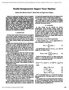
Fig. 1.

Artificial dataset with a linearly separable subclass structure.

skewness and kurtosis of the (i, j) subclass respectively, computed as follows βî,j = γî,j

Ni,j Ni,j 1 XX ˆ −1 (¯ ˆ i,j )T Σ ˆ i,j )]3 (14) [(¯ xκ − µ i,j xν − µ N 2 κ=1 ν=1

Ni,j 1 X ˆ −1 (¯ ˆ i,j )]2 ˆ i,j )T Σ [(¯ = xκ − µ i,j xκ − µ N κ=1

(15)

PNi,j ˆ i,j = 1 PNi,j (¯ ¯κ , Σ x where Ni,j , µ î,j = N1i,j κ=1 κ=1 xκ − Ni,j T ˆ i,j )(¯ ˆ i,j ) are the number of samples, the sample µ xκ − µ mean and the sample covariance matrix of (i, j) subclass, and the summands above are over the samples x ¯κ , x ¯ν that belong to the (i, j) subclass, i.e. the labels of the samples are (yν , uν ) = (yκ , uκ ) = (i, j). It has been shown in [10] that ˆ for large γi,j − F (F + p Ni,j , the quantities Ni,j βi,j /6 and (ˆ 2))/ 8F (F + 2)/Ni,j follow a chi-square distribution with F (F + 1)(F + 2)/6 degrees of freedom and a standard normal distribution N (0, 1) respectively. Consequently, Φi defined in (13) expresses the departure of the i-th class distribution from a multivariate Gaussian mixture. Using the iterative procedure described above, the best partition is selected using either cross-validation, i.e., we repeat the splitting procedure until a maximum number of subclasses is reached and then select the partition that provides the best empirical recognition rate, or by inspecting the convergence of a total nongaussianity measure Φ = Φ1 + Φ2 to a steady-state solution. We used the former approach in our experiments. III. E XPERIMENTAL RESULTS

In the above, we exploit a partitioning of the data to subclasses. Assuming that the data have a Gaussian subclass structure, we use an iterative algorithm to derive this subclass division. Starting from the initial class partition (i.e. H = 2), at each iteration we increase the number of subclasses of the kth class according to the following rule k = argmaxi=1,2 (Φi ), where Φi measures the nongaussianity of the i-th class. Exploiting the work in [10] we define this measure as ! Ã Hi X γî,j − F (F + 2) Ni,j βî,j + |p | , (13) Φi = 6 8F (F + 2)/Ni,j j=1 where F is the dimensionality of the feature vectors. The quantities βî,j , γî,j above are estimates of the multivariate

A. Artificial dataset A classification example with two non-linearly separable classes X1 , X2 is depicted in Figure 1. X1 consists of two Gaussian subclasses X1,1 , X1,2 , whereas X2 is a single Gaussian X2,1 . In contrary to the main classes, this dataset has a linearly separable subclass structure. From each subclass distribution 300 samples were randomly drawn to form the artificial dataset. The subclass partitioning (II-D) and the LSSVM algorithm were then applied, correctly identifying the subclass structure of the data and the separating hyperplanes η 1,1 , η 2,1 . For comparison, the hyperplane η svm computed by LSVM does not provide a valid solution for separating the two classes. At the same time, LSSVM avoids the unnecessary



computations for estimating the hyperplane that separates subclasses X1,1 and X1,2 , which MSVM would perform. B. UCI and Delve datasets We compare the performance of LSSVM with LSVM, KSVM with radial basis function (RBF) kernel [1], MLSVM [5], MixLSVM [2] and subclass ECOC (SECOC) [3], using 11 datasets from the UCI [11] and Delve [12] repositories: WDBC, Ionosphere, Breast Cancer, Pima, German, Heart, Splice, Titanic, and Monk-1,-2,-3. For the evaluation of the algorithms, a division of the datasets to training and test sets is necessary. This already exists for the Monk sets. For Ionosphere, similarly to other works, we use the first 200 samples for training and the rest 151 as testing instances, while, for WDBC we created a random 50–50 train–test split. For the Breast Cancer, Pima, German, Heart, Splice and Titanic datasets we used 10 random partitions for each dataset from the Gunnar Rätsch’s benchmark collection [13]. The recognition performance of a method regarding a dataset is measured using the average correct recognition rate (CCR) along all the partitions. Moreover, for assessing the statistical significance of the difference in the performance between any two algorithms, we used the McNemar’s hypothesis test [14]. For the experiments, LSSVM and MixLSVM were implemented in Matlab, while for LSVM, KSVM, MSVM and the base classifiers of SECOC, the libsvm [15] or the liblinear [16] packages were used. In SECOC, for fair comparison with LSSVM, we used LSVMs as base classifiers and the LLW strategy for classifying a test sample. In the stage of model selection, for LSVM we need to estimate the penalty term C, while for KSVM and LSSVM we additionally optimize over the scale parameter σ of the RBF function [1] and the number of subclasses H, respectively. Three parameters are optimized for MixLSVM, i.e, C, H and the scale parameter τ of the gating function [2]. Finally, in SECOC we search for the optimal values of the three splitting criteria (θsize , θperf and θimpr ) [3] and the penalty term C of the base classifiers. The optimal parameters for each method are selected through a grid search strategy where the primary metric is the CCR. The evaluation results are presented in Table I. We can see that LSSVM provides top recognition rate in 8 out of the 11 datasets. Using the McNemar’s test with significance level 0.025 we verified that the differences in performance between LSSVM and MSVM are statistically significant in 8 of the datasets; and similarly in 7 of the datasets for the differences between LSSVM and MixLSVM, and between LSSVM and SECOC. We experimentally verified that the training of LSSVM is much faster than MixLSVM (on average, 25 times faster) mainly due to the slow convergence of the expectation maximization-based MixLSVM, and because LSSVM requires the optimization of fewer training parameters; similarly, we expect the training stage of LSSVM to be faster than SECOC, due to the lower number of parameters that need to be optimized. The LSSVM training and testing are also less computationally demanding in comparison to MSVM and KSVM, due to the lower number of constraints and the absence of a kernel evaluation step, respectively.

Monk-1 Monk-2 Monk-3 WDBC Ionosph. B. Cancer Pima German Heart Splice Titanic

4

LSVM 70.6% 67.1% 81% 95.8% 97.4% 69.7% 76.9% 76.9% 81.7% 84.1% 76.6%

LSSVM 98.8% 75.5% 96.5% 96.1% 98.7% 77.9% 79% 79.7% 85.6% 89.6% 78.6%

MSVM 94.7% 74.5% 86.6% 95.4% 95.4% 72.6% 75.6% 74% 82.7% 88.6% 76.8%

MixLSVM 86.3% 76.9% 96.5% 96.1% 98% 74.6% 77.7% 76.9% 83.7% 87.5% 77.8%

SECOC 81.7% 67.3% 93% 96.1% 97.4% 74% 77.9% 80.3% 83.2% 88% 77.6%

KSVM 86.1% 81.9% 97% 94.4% 98% 74.7% 77% 77.9% 84.4% 88.4% 78%

TABLE I C ORRECT RECOGNITION RATES .

IV. C ONCLUSIONS In this letter, LSSVMs were proposed that exploit the subclass structure of the data to efficiently compute a separating piecewise linear hyperplane. Experiments on various datasets demonstrated the effectiveness of LSSVMs. ACKNOWLEDGMENT This work was supported by the EC under contracts FP7248984 GLOCAL and FP7-287911 LinkedTV. R EFERENCES [1] V. Vapnik, Statistical learning theory. New York: Willey, 1998. [2] Z. Fu, A. Robles-Kelly, and J. Zhou, “Mixing linear SVMs for nonlinear classification,” IEEE Trans. Neural Netw., vol. 21, no. 12, pp. 1963– 1975, Dec. 2010. [3] S. Escalera, D. M. Tax, O. Pujol, P. Radeva, and R. P. Duin, “Subclass problem-dependent design for error-correcting output codes,” IEEE Trans. Pattern Anal. Mach. Intell., vol. 30, no. 6, pp. 1041–1054, Jun. 2008. [4] S. Escalera, O. Pujol, and P. Radeva, “On the decoding process in ternary error-correcting output codes,” IEEE Trans. Pattern Anal. Mach. Intell., vol. 32, no. 1, pp. 120–134, Jan. 2010. [5] K. Crammer and Y. Singer, “On the algorithmic implementation of multiclass kernel-based vector machines,” J. Mach. Learn. Res., vol. 2, pp. 265–292, Mar. 2002. [6] Y. Guermeur, A. Elisseeff, and D. Zelus, “A comparative study of multiclass support vector machines in the unifying framework of large margin classifiers,” Appl. Stoch. Model. Bus. Ind., vol. 21, no. 2, pp. 199–214, Mar. 2005. [7] N. Gkalelis, V. Mezaris, and I. Kompatsiaris, “Mixture subclass discriminant analysis,” IEEE Signal Process. Lett., vol. 18, no. 5, pp. 319–322, May 2011. [8] S. S. Keerthi, S. Sundararajan, K.-W. Chang, C.-J. Hsieh, and C.-J. Lin, “A sequential dual method for large scale multi-class linear SVMs,” in Proc. 14th ACM SIGKDD, Las Vegas, USA, Aug. 2008, pp. 408–416. [9] E. J. Bredensteiner and K. P. Bennett, “Multicategory classification by support vector machines,” Comput. Optim. Appl., vol. 12, no. 1–3, pp. 53–79, Jan. 1999. [10] K. V. Mardia, “Measures of multivariate skewness and kurtosis with applications,” Biometrika, vol. 57, no. 3, pp. 519–530, Dec. 1970. [11] A. Frank and A. Asuncion, “UCI machine learning repository.” University of California, Irvine, School of Information and Computer Sciences, 2010. [Online]. Available: http://archive.ics.uci.edu/ml [12] “Data for evaluating learning in valid experiments,” http://www.cs. toronto.edu/∼delve/index.html, accessed 2012-06-10. [13] G. Rätsch, T. Onoda, and K.-R. Müller, “Soft margins for adaboost,” Mach. Learn., vol. 42, no. 3, pp. 287–320, Mar. 2001. [14] Q. McNemar, “Note on the sampling error of the difference between correlated proportions or percentages,” Psychometrika, vol. 12, no. 2, pp. 153–157, Jun. 1947. [15] C.-C. Chang and C.-J. Lin, “LIBSVM: A library for support vector machines,” ACM Trans. Intell. Syst. Technol., vol. 2, pp. 27:1–27:27, 2011. [16] R.-E. Fan, K.-W. Chang, C.-J. Hsieh, X.-R. Wang, and C.-J. Lin, “LIBLINEAR: A library for large linear classification,” Journal of Machine Learning Research, vol. 9, pp. 1871–1874, 2008.
