Mar 2, 2011 - network from Amazon.com data, social networks, email networks, a citation net- work, and two ..... Conference on Email and Anti-Spam (2004). 25. Knuth ... Leskovec, J., Adamic, L., Adamic, B.: The dynamics of viral marketing.
Listing All Maximal Cliques in Large Sparse Real-World Graphs David Eppstein and Darren Strash
arXiv:1103.0318v1 [cs.DS] 2 Mar 2011
Department of Computer Science, University of California, Irvine, USA.
Abstract. We implement a new algorithm for listing all maximal cliques in sparse graphs due to Eppstein, L¨offler, and Strash (ISAAC 2010) and analyze its performance on a large corpus of real-world graphs. Our analysis shows that this algorithm is the first to offer a practical solution to listing all maximal cliques in large sparse graphs. All other theoretically-fast algorithms for sparse graphs have been shown to be significantly slower than the algorithm of Tomita et al. (Theoretical Computer Science, 2006) in practice. However, the algorithm of Tomita et al. uses an adjacency matrix, which requires too much space for large sparse graphs. Our new algorithm opens the door for fast analysis of large sparse graphs whose adjacency matrix will not fit into working memory. Keywords: maximal clique listing, Bron–Kerbosch algorithm, sparse graphs, ddegenerate graphs
1
Introduction
Clique finding procedures arise in the solutions to a wide variety of important application problems. The problem of finding cliques was first studied in social network analysis, as a way of finding closely-interacting communities of agents in a social network [19]. In bioinformatics, clique finding procedures have been used to find frequently occurring patterns in protein structures [17,26,27], to predict the structures of proteins from their molecular sequences [43], and to find similarities in shapes that may indicate functional relationships between proteins [14]. Other applications of clique finding problems include information retrieval [5], computer vision [20], computational topology [50], and e-commerce [49]. For many applications, we do not want to report one large clique, but all maximal cliques. Any algorithm which solves this problem must take exponential time in the worst-case because graphs can contain an exponential number of cliques [37]. However, graphs with this worst-case behavior are not typically encountered in practice. More than likely, the types of graphs that we will encounter are sparse [16]. Therefore, the feasibility of clique listing algorithms lies in their ability to appropriately handle sparse input graphs. Indeed, it has long been known that certain sparse graph families, such as planar graphs and graphs with low arboricity, contain only a linear number of cliques, and that all maximal cliques in these graphs can be listed in linear time [10,11]. In addition, there are also several methods to list all cliques in time polynomial in the number of cliques reported [46], which can be done faster if parameterized on a sparsity measure such as maximum degree [36].
Many different clique-finding algorithms have been implemented, and an algorithm of Tomita et al. [45], based on the much earlier Bron–Kerbosch algorithm [8], has been shown through many experiments to be faster by orders of magnitude in practice than others. An unfortunate drawback of the algorithm of Tomita et al., however, is that both its theoretical analysis and implementation rely on the use of an adjacency matrix representation of the input graph. For this reason, their algorithm has limited applicability for large sparse graphs, whose adjacency matrix may not fit into working memory. We therefore seek to have the best of both worlds: we would ideally like an algorithm that rivals the speed of the Tomita et al. result, while having linear storage cost. Recently, together with Maarten L¨offler, the authors developed and published a new algorithm for listing maximal cliques, particularly optimized for the case that the input graph is sparse [13]. This new algorithm combines features of both the algorithm of Tomita et al. and the earlier Bron–Kerbosch algorithm on which it was based, and maintains through its recursive calls a dynamic graph data structure representing the adjacencies between the vertices that remain relevant within each call. When analyzed using parameterized complexity in terms of the degeneracy of the input graph (a measure of its sparsity) its running time is near-optimal in terms of the worst-case number of cliques that a graph with the same sparsity could have. However, the previous work of the authors with L¨offler did not include any implementation or experimental results showing the algorithm to be good in practice as well as in theory. 1.1
Our Results
We implement the algorithm of Eppstein, L¨offler, and Strash for listing all maximal cliques in sparse graphs [13]. Using a corpus of many large real-world graphs, together with synthetic data including the Moon–Moser graphs as well as random graphs, we compare the performance of our implementation with the algorithm of Tomita et al. We also implement for comparison, a modified version of the Tomita et al. algorithm that uses adjacency lists in place of adjacency matrices, and a simplified version of the Eppstein–L¨offler–Strash algorithm that represents its subproblems as lists of vertices instead of as dynamic graphs. Our results show that, for large sparse graphs, the new algorithm is as fast or faster than Tomita et al., and sometimes faster by very large factors. For graphs that are not as sparse, the new algorithm is sometimes slower than the algorithm of Tomita et al., but remains within a small constant factor of its performance.
2
Preliminaries
We work with an undirected graph G = (V, E) with n vertices and m edges. For a vertex v, let Γ (v) be itsTneighborhood {w | (v, w) ∈ E}, and similarly for a subset W ⊂ V let Γ (W ) be the set w∈W Γ (w), the common neighborhood of all vertices in W . 2.1
Degeneracy
Definition 1 (degeneracy). The degeneracy of a graph G is the smallest number d such that every subgraph of G contains a vertex of degree at most d.
proc Tomita(P, R, X) 1: if P ∪ X = 0/ then 2: report R as a maximal clique 3: end if 4: choose a pivot u ∈ P ∪ X to maximize |P ∩ Γ (u)| 5: for each vertex v ∈ P \ Γ (u) do 6: Tomita(P ∩ Γ (v), R ∪ {v}, X ∩ Γ (v)) 7: P ← P \ {v} 8: X ← X ∪ {v} 9: end for Fig. 1. The Bron–Kerbosch algorithm with the pivoting strategy of Tomita et al.
Every graph with degeneracy d has a degeneracy ordering, a linear ordering of the vertices such that each vertex has at most d neighbors later than it in the ordering. The degeneracy of a given graph and a degeneracy ordering of the graph can both be computed in linear time [6]. 2.2
The Algorithm of Tomita et al.
The algorithm of Tomita et al. [45] is an implementation of Bron and Kerbosch’s algorithm [8], using a heuristic called pivoting [26,9]. The Bron–Kerbosch algorithm is a simple recursive algorithm that maintains three sets of vertices: a partial clique R, a set of candidates for clique expansion P, and a set of forbidden vertices X. In each recursive call, a vertex v from P is added to the partial clique R, and the sets of candidates for expansion and forbidden vertices are restricted to include only neighbors of v. If P ∪ X becomes empty, the algorithm reports R as a maximal clique, but if P becomes empty while X is nonempty, the algorithm backtracks without reporting a clique. In the basic version of the algorithm, |P| recursive calls are made, one for each vertex in P. The pivoting heuristic reduces the number of recursive calls by choosing a vertex u in P ∪ X called a pivot. All maximal cliques must contain a non-neighbor of u (counting u itself as a non-neighbor), and therefore, the recursive calls can be restricted to the intersection of P with the non-neighbors. The algorithm of Tomita et al. chooses the pivot so that u has the maximum number of neighbors in P, and therefore the minimum number of non-neighbors, among all possible pivots. Computing both the pivot and the vertex sets for the recursive calls can be done in time O(|P| · (|P| + |X|)) within each call to the algorithm, using an adjacency matrix to quickly test the adjacency of pairs of vertices. This pivoting strategy, together with this adjacency-matrix-based method for computing the pivots, leads to a worstcase time bound of O(3n/3 ) for listing all maximal cliques [45]. 2.3
The Algorithm of Eppstein, L¨offler, and Strash
Eppstein, L¨offler, and Strash [13] provide a different variant of the Bron–Kerbosch algorithm that obtains near-optimal worst-case time bounds for graphs with low degeneracy. They first compute a degeneracy ordering of the graph; the outermost call in the
proc Degeneracy(V , E) 1: for each vertex vi in a degeneracy ordering v0 , v1 , v2 , . . . of (V, E) do 2: P ← Γ (vi ) ∩ {vi+1 , . . . , vn−1 } 3: X ← Γ (vi ) ∩ {v0 , . . . , vi−1 } 4: Tomita(P, {vi }, X) 5: end for Fig. 2. The algorithm of Eppstein, L¨offler, and Strash.
recursive algorithm selects the vertices v to be used in each recursive call, in this order, without pivoting. Then for each vertex v in the order, a call is made to the algorithm of Tomita et al. [45] to compute all cliques containing v and v’s later neighbors, while avoiding v’s earlier neighbors. The degeneracy ordering limits the size of P within these recursive calls to be at most d, the degeneracy of the graph. A simple strategy for determining the pivots in each call to the algorithm of Tomita et al., used as a subroutine within this algorithm, would be to loop over all possible pivots in X ∪P and, for each one, loop over its later neighbors in the degeneracy ordering to determine how many of them are in P. The same strategy can also be used to perform the neighbor intersection required for recursive calls. With the pivot selection and set intersection algorithms implemented in this way, the algorithm would have running time O(d 2 n3d/3 ), a factor of d larger than the worst-case output size, which is O(d(n − d)3n/3 ). However, Eppstein et al. provide a refinement of this algorithm that stores, at each level of the recursion, the subgraph of G with vertices in P ∪ X and edges having at least one endpoint in P. Using this subgraph, they reduce the pivot computation time to |P|(|X| + |P|), and the neighborhood intersection for each recursive call to time |P|2 (|X| + |P|), which reduces the total running time to O(dn3d/3 ). This running time matches the worst-case output size of the problem whenever d ≤ n−Ω (n). As described by Eppstein et al., storing the subgraphs at each level of the recursion may require as much as O(dm) space. But as we show in Section 3.1, it is possible to achieve the same optimal running time with space overhead O(n + m). 2.4
Tomita et al. with Adjacency Lists
In our experiments, we were only able to run the algorithm of Tomita et al. [45] on graphs of small to moderate size, due to its use of the adjacency matrix representation. In order to have a basis for comparison with this algorithm on larger graphs, we also implemented a simple variant of the algorithm which stores the input graph in an adjacency list representation, and which performs the pivot computation by iterating over all vertices in P ∪ X and testing all neighbors for membership in P. When a vertex v is added to R for a recursive call, we can intersect the neighborhood of r with P and X by iterating over its neighbors in the same way. Let ∆ be the maximum degree of the given input graph; then the pivot computation takes time (O∆ (|X| + |P|)). Additionally, preparing subsets for all recursive calls takes time O(|P|∆ ). Fitting these facts into the analysis of Tomita et al. gives us a
O(∆ (n − ∆ )3∆ /3 ) time algorithm. ∆ may be significantly larger than the degeneracy, so this algorithm’s theoretical time bounds are not as good as those of Tomita et al. or Eppstein et al.; nevertheless, the simplicity of this algorithm makes it competitive with the others for many problem instances.
3
Implementation and experiments
We implemented the algorithm of Tomita et al. using the adjacency matrix representation, and the simple adjacency list representation for comparison. We also implemented three variants of the algorithm of Eppstein, L¨offler, and Strash: one with no data structuring, using the fact that vertices have few later neighbors in the degeneracy ordering, an implementation of the dynamic graph data structure that only uses O(m + n) extra space total, and an alternative implementation of the data structure based on bit vectors. The bit vector implementation executed no faster than the data structure implementation, so we omit its experimental timings and any discussion of its implementation details. 3.1
Implementation Details
We maintain the sets of vertices P and X in a single array, which is passed between recursive calls. Initially, the array contains the elements of X followed by the elements of P. We keep a reverse lookup table, so that we can look up the index of a vertex in constant time. With this lookup table, we can tell whether a vertex is in P or X in constant time, by testing that its index is in the appropriate subarray. When a vertex v is added to R in preparation for a recursive call, we reorder the array. Vertices in Γ (v) ∩ X are moved to the end of the X subarray, and vertices in Γ (v) ∩ P are moved to the beginning of the P subarray (see Figure 3). We then make a recursive call on the subarray containing the vertices Γ (v) ∩ (X ∪ P). After the recursive call, we move v to X by swapping it to the beginning of the P subarray and moving the boundary so that v is in the X subarray. Of course, moving vertices between sets will affect P and X in higher recursive calls. Therefore, in a given recursive call, we maintain a list of the vertices that are moved from P to X, and move these vertices back to P when the call ends.
1
8
3 12 7
6
X
9
P
4
2 11 10
6
8
3
7 12 1
X ∩ Γ(v)
2 11 9
4 10
P ∩ Γ(v)
Fig. 3. When a vertex v is added to the partial clique R, its neighbors in P and X (highlighted in this example) are moved toward the dividing line in preparation for the next recursive call.
6
8
3
7 12 1
2 11 9
9 2 4 11
9 4 2 10 9 11 9 4 11 4 2 11 9 4 2 9 4
4 10
6
8
3
7 12 1
2 11 9
2 11 4 9
11 11 2 11 2 2 9 4 10 4 9 4 9 4 9 9 4
4 10
Fig. 4. For each vertex in P ∪ X, we keep an array containing neighbors in P. We update these arrays whenever a vertex is moved from P to R, and whenever we need to intersect a neighborhood with P and X for a recursive call.
The pivot computation data structure is stored as set of arrays, one for each potential pivot vertex u in P ∪ X, containing the neighbors of u in P. Whenever P changes, we reorder the elements in these arrays so that neighbors in P are stored first (see Figure 4). Computing the pivot is as simple as iterating through each array until we encounter a neighbor that is not in P. This reordering procedure allows us to maintain one set of arrays throughout all recursive calls, requiring linear space total. Making a new copy of this data structure for each recursive call would require space O(dm). 3.2
Results
We implemented all algorithms in the C programming language, and ran experiments on a Linux workstation running the 32-bit version of Ubuntu 10.10, with a 2.53 GHz Intel Core i5 M460 processor (with three cache levels of 128KB, 512KB, and 3,072KB respectively) and 2.6GB of memory. We compiled our code with version 4.4.5 of the gcc compiler with the -O2 optimization flag. In our tables of results, “tomita” is the algorithm of Tomita et al., “maxdegree” is the simple implementation of Tomita et al.’s algorithm for adjacency lists, and “hybrid” and “degen” are the implementations of Eppstein, L¨offler, and Strash with no data structure and with the linear space data structure, respectively. We provide the elapsed running running times (in seconds) for each of these algorithms; an asterisk indicates that the algorithm was unable to run on that problem instance due to time or space limitations. In addition, we list the number of vertices n, edges m, the degeneracy d, and the number of maximal cliques µ. Our primary experimental data consisted of four publicly-available databases of real-world networks, including non-electronic and electronic social networks as well as networks from bioinformatics applications. – A data base curated by Mark Newman [40] (Table 1) which consists primarily of social networks; it also includes word co-occurrence data and a biological neural network. Many of its graphs were too small for us to time our algorithms accurately, but our algorithm was faster than that of Tomita et al. on all four of the largest graphs; in one case it was faster by a factor of approximately 130.
– The BioGRID data [44] (Table 2) consists of several protein-protein interaction networks with from one to several thousand vertices, and varying sparsities. Our algorithm was significantly faster than that of Tomita et al. on the worm and fruitfly networks, and matched or came close to its performance on all the other networks, even the relatively dense yeast network. – We also tested six large social and bibliographic networks that appeared in the Pajek data set but were not in the other data sets [7] (Table 3). Our algorithm was consistently faster on these networks. Due to their large size, the algorithm of Tomita et al. was unable to run on two of these networks; nevertheless, our algorithm found all cliques quickly in these graphs. – We also tested a representative sample of graphs from the Stanford Large Network Dataset Collection [32] (Table 4). These included road networks, a co-purchasing network from Amazon.com data, social networks, email networks, a citation network, and two Web graphs. Nearly all of these input graphs were too large for the Tomita et al. algorithm to fit into memory. For graphs which are extremely sparse, it is no surprise that the maxdegree algorithm was faster than our algorithm, but our algorithm was consistently fast on each of these data sets, whereas the maxdegree algorithm was orders of magnitude slower than our algorithm on the large soc-wiki-Talk network.
Table 1. Experimental results for Mark Newman’s data sets [40] graph n m d µ zachary [48] 34 78 4 39 dolphins [35] 62 159 4 84 power [47] 4,941 6,594 5 5,687 polbooks [28] 105 441 6 199 adjnoun [29] 112 425 6 303 football [15] 115 613 8 281 lesmis [25] 77 254 9 59 celegensneural [47] 297 1,248 9 856 netscience [39] 1,589 2,742 19 741 internet [40] 22,963 48,421 25 39,275 condmat-2005 [38] 40,421 175,693 29 34,274 polblogs [4] 1,490 16,715 36 49,884 astro-ph [38] 16,706 121,251 56 15,794
tomita maxdegree hybrid degen < 0.01 < 0.01 < 0.01 < 0.01 < 0.01 < 0.01 < 0.01 < 0.01 0.29 < 0.01 0.01 0.01 < 0.01 < 0.01 < 0.01 < 0.01 < 0.01 < 0.01 < 0.01 < 0.01 < 0.01 < 0.01 < 0.01 < 0.01 < 0.01 < 0.01 < 0.01 < 0.01 < 0.01 < 0.01 < 0.01 < 0.01 0.02 < 0.01 < 0.01 < 0.01 6.68 0.28 0.11 0.11 39.65 0.22 0.32 0.35 0.08 0.28 0.18 0.12 3.44 0.19 0.22 0.23
As a reference point, we also ran our experimental comparisons using the two sets of graphs that Tomita et al. used in their experiments. First, Tomita et al. used a data set from a DIMACS challenge, a collection of graphs that were intended as difficult examples for clique-finding algorithms, and that have been algorithmically generated (Table 5). And second, they generated graphs randomly with varying edge densities; in order to replicate their results we generated another set of random graphs with the same parameters (Table 6). The algorithm of Eppstein, L¨offler, and Strash runs about
Table 2. Experimental results for BioGRID data sets (PPI Networks)[44]. graph mouse worm plant fruitfly human fission-yeast yeast
n m 1,455 1,636 3,518 3,518 1,745 3,098 7,282 24,894 9,527 31,182 2,031 12,637 6,008 156,945
d µ tomita maxdegree hybrid degen 6 1,523 0.01 < 0.01 < 0.01 < 0.01 10 5,652 0.14 0.01 0.01 0.01 12 2,302 0.02 < 0.01 < 0.01 < 0.01 12 21,995 0.62 0.03 0.03 0.04 12 23,863 1.06 0.03 0.05 0.05 34 28,520 0.06 0.12 0.09 0.07 64 738,613 1.74 11.37 4.22 2.17
Table 3. Experimental results for Pajek data sets [7]. graph n m d µ tomita maxdegree hybrid degen foldoc [21] 13,356 91,471 12 39,590 2.16 0.11 0.14 0.13 eatRS [23] 23,219 304,937 34 298,164 7.62 1.52 1.55 1.03 hep-th [3] 27,240 341,923 37 446,852 12.56 3.40 2.40 1.70 patents [18] 240,547 560,943 24 482,538 * 0.56 1.22 1.65 days-all [12] 13,308 148,035 73 2,173,772 5.83 62.86 9.94 5.18 ND-www [1] 325,729 1,090,108 155 495,947 * 1.80 1.81 2.12
Table 4. Experimental results for Stanford data sets [32]. graph roadNet-CA [34] roadNet-PA [34] roadNet-TX [34] amazon0601 [30] email-EuAll [31] email-Enron [24] web-Google [2] soc-wiki-Vote [33] soc-slashdot0902 [34] cit-Patents [18] soc-Epinions1 [42] soc-wiki-Talk [33] web-berkstan [34]
n 1,965,206 1,088,092 1,379,917 403,394 265,214 36,692 875,713 7,115 82,168 3,774,768 75,888 2,394,385 685,231
m 2,766,607 1,541,898 1,921,660 2,443,408 364,481 183,831 4,322,051 100,762 504,230 16,518,947 405,740 4,659,565 6,649,470
d 3 3 3 10 37 43 44 53 55 64 67 131 201
µ tomita maxdegree 2,537,996 * 2.00 1,413,391 * 1.09 1,763,318 * 1.35 1,023,572 * 3.59 265,214 * 4.93 226,859 31.96 2.78 1,417,580 * 9.01 459,002 0.96 4.21 890,041 * 7.81 14,787,032 * 28.56 1,775,074 * 27.87 86,333,306 * > 18, 000 3,405,813 * 76.90
hybrid 5.34 2.95 3.72 5.01 1.25 1.30 8.43 2.10 4.20 49.22 9.24 542.28 31.81
degen 5.81 3.21 4.00 6.03 1.33 0.90 9.70 1.14 2.58 58.64 4.78 216.00 20.87
2 to 3 times slower than that of Tomita et al. on many of these graphs; this confirms that the algorithm is still competitive on graphs that are not sparse, in contrast to the competitors in Tomita et al.’s paper which ran 10 to 160 times slower on these input graphs. The largest of the random graphs in the second data set were generated with edge probabilities that made them significantly sparser than the rest of the set; for those graphs our algorithm outperformed that of Tomita et al by a factor that was as large
as 30 on the sparsest of the graphs. The maxdegree algorithm was even faster than our algorithm in these cases, but it was significantly slower on other data. Table 5. Experimental results for Moon–Moser [37] and DIMACS benchmark graphs [22]. Graphs M-M-30 M-M-45 M-M-48 M-M-51 MANN a9 brock 200 2 c-fat200-5 c-fat500-10 hamming6-2 hamming6-4 johnson8-4-4 johnson16-2-4 keller4 p hat300-1 p hat300-2
4
n m d µ tomita maxdegee hybrid degen 30 405 27 59,049 0.04 0.04 0.06 0.04 45 945 42 14,348,907 7.50 15.11 20.36 10.21 48 1080 45 43,046,721 22.52 48.37 63.07 30.22 51 1224 48 129,140,163 67.28 150.02 198.06 91.80 45 918 27 590,887 0.44 0.88 0.90 0.53 200 9876 84 431,586 0.55 2.95 2.61 1.22 200 8473 83 7 0.01 0.01 0.01 0.01 500 46627 185 8 0.04 0.04 0.09 0.12 64 1824 57 1,281,402 1.36 4.22 4.15 2.28 64 704 22 464 < 0.01 < 0.01 < 0.01 < 0.01 70 1855 53 114,690 0.13 0.35 0.40 0.24 120 5460 91 2,027,025 5.97 27.05 31.04 12.17 171 9435 102 10,284,321 5.98 24.97 26.09 11.53 300 10933 49 58,176 0.07 0.29 0.25 0.15 300 21928 98 79,917,408 91.31 869.34 371.72 163.16
Conclusion
We have shown that the algorithm of Eppstein, L¨offler, and Strash is a practical algorithm for large sparse graphs. This algorithm is highly competitive with the algorithm of Tomita et al. on sparse graphs, and within a small constant factor on other graphs. The advantage of this algorithm is that it requires only linear space for storing the graph and all data structures. It does not suffer from the drawback of requiring an adjacency matrix, which may not fit into memory. Its closest competitor in this respect, the Tomita et al. algorithm modified to use adjacency lists, is sometimes faster by a small factor but is also sometimes slower by a large factor. Thus, the algorithm of Eppstein et al. is a fast and reliable choice for listing maximal cliques, especially when the input graphs are large and sparse. For future work, it would be interesting to compare our results with those of other ¨ popular clique listing algorithms. We attempted to include results from Patric Osterg˚ ard’s popular Cliquer program [41] in our tables; however, at the time of writing, its newly implemented functionality for listing all maximal cliques returns incorrect results. Acknowledgments We thank Etsuji Tomita and Takeaki Uno for helpful discussions. This research was supported in part by the National Science Foundation under grant 0830403, and by the Office of Naval Research under MURI grant N00014-08-1-1015.
Table 6. Experimental results on random graphs. Graphs n p 0.6 0.7 100 0.8 0.9
d
µ tomita maxdegree
51 59,898 0.08 59 439,928 0.50 70 5,776,276 6.29 81 240,998,654 249.15 3,663 < 0.01 18,911 0.02 86,179 0.10 555,724 0.70 4,151,668 5.59 72,454,791 101.35
hybrid
degen
0.26 0.25 0.14 2.04 1.85 0.99 28.00 24.86 11.74 1136.15 1028.84 425.85
300
21 47 74 101 130 162
500
0.1 0.2 0.3 0.5
39 15,311 0.02 81 98,875 0.11 127 701,292 0.86 225 103,686,974 151.67
0.1 0.2 0.3
56 117 184
38,139 321,245 3,107,208
0.04 0.37 4.06
0.10 2.01 36.13
0.19 2.69 38.12
0.09 1.00 11.47
1,000
0.1 0.2 0.3
82 172 266
99,561 1,190,899 15,671,489
0.11 1.45 21.96
0.34 10.35 262.64
0.70 14.48 280.58
0.28 4.33 66.05
2,000
0.1
170
750,991
1.05
5.18
11.77
3.13
3,000
0.1
263
2,886,628
4.23
27.51
68.52
13.62
0.001 7 0.003 21 10,000 0.005 38 0.01 80 0.03 262
49,716 141,865 215,477 349,244 3,733,699
1.19 1.30 1.47 2.20 9.96
0.04 0.11 0.25 1.01 20.66
0.07 0.36 1.03 5.71 133.94
0.07 0.26 0.51 1.66 20.67
700
0.01 0.07 0.44 4.24 42.37 958.74
0.01 < 0.01 0.08 0.05 0.49 0.24 3.97 1.67 36.35 13.05 755.86 227.00
0.1 0.2 0.3 0.4 0.5 0.6
0.03 0.06 0.04 0.46 0.61 0.27 5.90 6.10 2.29 1888.20 1521.90 375.23
References 1. Self-organized networks database, University of Notre Dame 2. Google programming contest (2002), http://www.google.com/ programming-contest/ 3. Kdd cup (2003), http://www.cs.cornell.edu/projects/kddcup/index. html 4. Adamic, L.A., Glance, N.: The political blogosphere and the 2004 us election. In: Proceedings of the WWW-2005 Workshop on the Weblogging Ecosystem (2005)
5. Augustson, J.G., Minker, J.: An analysis of some graph theoretical cluster techniques. J. ACM 17(4), 571–588 (1970) 6. Batagelj, V., Zaverˇsnik, M.: An O(m) algorithm for cores decomposition of networks (2003), http://arxiv.org/abs/cs.DS/0310049 7. Batagelj, V., Mrvar, A.: Pajek datasets (2006), http://vlado.fmf.uni-lj.si/ pub/networks/data/ 8. Bron, C., Kerbosch, J.: Algorithm 457: finding all cliques of an undirected graph. Commun. ACM 16(9), 575–577 (1973) 9. Cazals, F., Karande, C.: A note on the problem of reporting maximal cliques. Theor. Comput. Sci. 407(1-3), 564 – 568 (2008) 10. Chiba, N., Nishizeki, T.: Arboricity and subgraph listing algorithms. SIAM J. Comput. 14(1), 210–223 (1985) 11. Chrobak, M., Eppstein, D.: Planar orientations with low out-degree and compaction of adjacency matrices. Theor. Comput. Sci. 86(2), 243 – 266 (1991) 12. Corman, S.R., Kuhn, T., Mcphee, R.D., Dooley, K.J.: Studying complex discursive systems: Centering resonance analysis of communication. Human Communication Research 28(2), 157–206 (2002) 13. Eppstein, D., L¨offler, M., Strash, D.: Listing all maximal cliques in sparse graphs in nearoptimal time. In: Cheong, O., Chwa, K.Y., Park, K. (eds.) ISAAC 2010, LNCS, vol. 6506, pp. 403–414. Springer-Verlag (2010) 14. Gardiner, E.J., Willett, P., Artymiuk, P.J.: Graph-theoretic techniques for macromolecular docking. J. Chem. Inf. Comput. Sci. 40(2), 273–279 (2000) 15. Girvan, M., Newman, M.E.J.: Community structure in social and biological networks. Proc. Natl. Acad. Sci. USA 99, 7821–7826 (2002) 16. Goel, G., Gustedt, J.: Bounded arboricity to determine the local structure of sparse graphs. In: Fomin, F. (ed.) WG 2006. LNCS, vol. 4271, pp. 159–167. Springer-Verlag (2006) 17. Grindley, H.M., Artymiuk, P.J., Rice, D.W., Willett, P.: Identification of tertiary structure resemblance in proteins using a maximal common subgraph isomorphism algorithm. J. Mol. Biol. 229(3), 707 – 721 (1993) 18. Hall, B.H., Jaffe, A.B., Trajtenberg, M.: The NBER patent citation data file: Lessons, insights and methodological tools. Tech. rep. (2001), NBER Working Paper 8498 19. Harary, F., Ross, I.C.: A procedure for clique detection using the group matrix. Sociometry 20(3), 205–215 (1957) 20. Horaud, R., Skordas, T.: Stereo correspondence through feature grouping and maximal cliques. IEEE Trans. Patt. An. Mach. Int. 11(11), 1168–1180 (1989) 21. Howe, D.: Foldoc: Free on-line dictionary of computing, http://foldoc.org/ 22. Johnson, D.J., Trick, M.A. (eds.): Cliques, Coloring, and Satisfiability: Second DIMACS Implementation Challenge, Workshop, October 11-13, 1993. American Mathematical Society, Boston, MA, USA (1996) 23. Kiss, G., Armstrong, C., Milroy, R., , Piper, J.: An associative thesaurus of English and its computer analysis. In: Aitken A.J., Bailey, R., Hamilton-Smith, N. (eds.) The Computer and Literary Studies. Edinburgh: University Press (1973) 24. Klimt, B., Yang, Y.: Introducing the enron corpus. In: CEAS 04: Proceedings of the 1st Conference on Email and Anti-Spam (2004) 25. Knuth, D.E.: The Stanford GraphBase: A Platform for Combinatorial Computing. AddisonWesley, Reading, MA (1993) 26. Koch, I.: Enumerating all connected maximal common subgraphs in two graphs. Theor. Comput. Sci. 250(1-2), 1 – 30 (2001) 27. Koch, I., Lengauer, T., Wanke, E.: An algorithm for finding maximal common subtopologies in a set of protein structures. J. Comput. Biol. 3(2), 289–306 (1996)
28. Krebs, V.: http://www.orgnet.com/, unpublished 29. Leicht, E.A., Holme, P., Newman, M.E.J.: Vertex similarity in networks. Phys. Rev. E 73 (2006) 30. Leskovec, J., Adamic, L., Adamic, B.: The dynamics of viral marketing. ACM Transactions on the Web 1(1) (2007) 31. Leskovec, J., Kleinberg, J., Faloutsos, C.: Graph evolution: Densification and shrinking diameters. ACM Transactions on Knowledge Discovery from Data 1(1) (2007) 32. Leskovec, J.: Stanford large network dataset collection, http://snap.stanford. edu/data/index.html 33. Leskovec, J., Huttenlocher, D., Kleinberg, J.: Predicting positive and negative links in online social networks. In: Proc. 19th Int. Conf. on World Wide Web. pp. 641–650. WWW ’10, ACM (2010) 34. Leskovec, J., Lang, K.J., Dasgupta, A., Mahoney, M.W.: Community structure in large networks: Natural cluster sizes and the absence of large well-defined clusters. Internet Mathematics 6(1), 29–123 (2009) 35. Lusseau, D., Schneider, K., Boisseau, O.J., Haase, P., Slooten, E., Dawson, S.M.: The bottlenose dolphin community of doubtful sound features a large proportion of long-lasting associations. Behavioral Ecology and Sociobiology 54, 396–405 (2003) 36. Makino, K., Uno, T.: New algorithms for enumerating all maximal cliques. In: Proc. 9th Scand. Worksh. Algorithm Theory. LNCS, vol. 3111, pp. 260–272. Springer-Verlag (2004) 37. Moon, J.W., Moser, L.: On cliques in graphs. Israel J. Math. 3(1), 23–28 (1965) 38. Newman, M.E.J.: The structure of scientific collaboration networks. Proc. Natl. Acad. Sci. USA 98, 404–409 (2001) 39. Newman, M.E.J.: Finding community structure in networks using the eigenvectors of matrices. Phys. Rev. E 74(3), 036104 (2006) 40. Newman, M.E.J.: http://www-personal.umich.edu/˜mejn/netdata/ ¨ 41. Niskanen, S., Osterg˚ ard, P.R.J.: Cliquer user’s guide, version 1.0. Tech. Rep. T48, Helsinki University of Technology (2003) 42. Richardson, M., Agrawal, R., Domingos, P.: Trust management for the semantic web. In: ISWC (2003) 43. Samudrala, R., Moult, J.: A graph-theoretic algorithm for comparative modeling of protein structure. J. Mol. Biol. 279(1), 287 – 302 (1998) 44. Stark, C., Breitkreutz, B.J., Reguly, T., Boucher, L., Breitkreutz, A., Tyers, M.: BioGRID: a general repository for interaction datasets. Nucleic Acids Res. 34, D535–D539 (2006) 45. Tomita, E., Tanaka, A., Takahashi, H.: The worst-case time complexity for generating all maximal cliques and computational experiments. Theor. Comput. Sci. 363(1), 28–42 (2006) 46. Tsukiyama, S., Ide, M., Ariyoshi, H., Shirakawa, I.: A new algorithm for generating all the maximal independent sets. SIAM J. Comput. 6(3), 505–517 (1977) 47. Watts, D.J., Strogatz, S.H.: Collective dynamics of ‘small-world’ networks. Nature 393, 440– 442 (1998) 48. Zachary, W.W.: An information flow model for conflict and fission in small groups. J. Anthropol. Res. 33, 452–473 (1977) 49. Zaki, M.J., Parthasarathy, S., Ogihara, M., Li, W.: New algorithms for fast discovery of association rules. In: Proc. 3rd Int. Conf. Knowledge Discovery and Data Mining. pp. 283–286. AAAI Press (1997), http://www.aaai.org/Papers/KDD/1997/KDD97-060. pdf 50. Zomorodian, A.: The tidy set: a minimal simplicial set for computing homology of clique complexes. In: Proc. 26th ACM Symp. Computational Geometry. pp. 257–266 (2010), http://www.cs.dartmouth.edu/˜afra/papers/socg10/tidy-socg.pdf