We have used LiteLab for many different kinds of network experiments and are ... scale real-world experiments requires a lot of resources. Vir- tualization may ...
LiteLab: Efficient Large-scale Network Experiments Liang Wang, Jussi Kangasharju
arXiv:1311.7422v1 [cs.DC] 28 Nov 2013
Department of Computer Science, University of Helsinki, Finland
Abstract—Large-scale network experiments is a challenging problem. Simulations, emulations, and real-world testbeds all have their advantages and disadvantages. In this paper we present LiteLab, a light-weight platform specialized for largescale networking experiments. We cover in detail its design, key features, and architecture. We also perform an extensive evaluation of LiteLab’s performance and accuracy and show that it is able to both simulate network parameters with high accuracy, and also able to scale up to very large networks. LiteLab is flexible, easy to deploy, and allows researchers to perform large-scale network experiments with a short development cycle. We have used LiteLab for many different kinds of network experiments and are planning to make it available for others to use as well.
I. I NTRODUCTION For network researchers, large-scale experiment is an important tool to test distributed systems. A system may exhibit quite different characteristics in a complex network as opposed to behavior observed in small-scale experiments. Thorough experimental evaluation before real-life deployment is very useful in anticipating problems. This means that the system should be tested with various parameter values, like different network topologies, bandwidths, link delays, loss rates and so on. It is also useful to see how the system interacts with other protocols, e.g. routers with different queueing policies. Due to the large parameter space, researchers usually need to run thousands of experiments with different parameter combinations. As Eide pointed out in [1], replayability is critical in modern network experiments. Not being able to replay an experiment implies the results are not reproducible, which makes it difficult to evaluate a system, because the results from different experiments are not comparable. A simulator has been a popular option due to its simplicity and controllability. It also has other benefits like reproducible results and low resource requirements. However, a simulator is only as good as the models used. Choosing the right granularity of abstraction is a tradeoff between more realistic results and increased computational complexity. Experiments on real systems can overcome many problems of simulators, because all the traffic flows through a real network with real-world behavior. However, running largescale real-world experiments requires a lot of resources. Virtualization may help, but configuring and managing large experiments is still difficult. Recently, high performance clusters are becoming common, virtualization technology advances, and overlay networks seem to become the de facto paradigm for modern distributed
systems. All these emerging technologies change the way we build and evaluate networked systems. In this paper, we present LiteLab, our flexible platform for large-scale networking experiments. We show its design, functionalities, key features and an evaluation of its accuracy and performance. With LiteLab, researchers can easily construct complex network on a resource-limited infrastructure. LiteLab is easy to configure and extend. Each router and links between them can be configured individually. New queueing policies, caching strategies and other network models can be added in without modifying existing code. The flexible design enables LiteLab to simulate both routers and end systems in the network. Researchers can easily plug in user application and study system behaviors. LiteLab takes advantages of overlay network techniques, providing a flexible experiment platform with many uses. It helps researchers reduce the experiment complexity and speeds up experiment life-cycle, and at the same time, provides satisfying accuracy. The organization of this paper is as follows. Section II discusses choices and existing solutions for network experiment platforms. Section III shows the design of LiteLab and its key features. We evaluate our platform and also provide some use cases in Section IV. We conclude the paper in Section V. II. BACKGROUND There are generally two methodologies to evaluate a system: model-based evaluation and experiment-based evaluation. The first tries to derive numeric performance values by applying analytical models. However, as the systems become larger and more distributed, system analysis becomes more complex. In most cases, it is impossible to build a mathematically tractable model. Experiment-based evaluation tackles this problem and we can identify three main forms of experiment-based evaluation: simulation, emulation, and real network testbeds. Below we present examples of these and discuss their pros and cons. After presenting LiteLab, we return to a comparison between LiteLab and the approaches below in Section IV-F. A. Simulator: NS2 and NS3 NS2 [2] is one of the most famous among general purpose simulators [2], [3]. It provides lots of models for many kinds of network settings. Users can implement their own model in C++ and plug it into NS2. Experiment configuration and deployment are done with Tcl/Tk scripts. NS3 has more features and tunable parameters to allow more realistic settings. However, increased complexity and detailed models significantly increase computational overheads.
2
Fig. 1: LiteLab Architecture
B. Emulator: Emulab Emulab [4] tries to integrate simulation, emulation and live network into a common framework. The aim is to combine the control and ease of use from simulation to emulation with the realism from live network. Users can configure the topology according to the experiment needs. The multiplexed virtual nodes are implemented with OpenVZ, a container-based virtualization scheme. Emulab uses VLAN and Dummynet [5] to emulate wide-area links within the local-area network. It is also able to mix traffic from Internet, NS3 and emulated links together. Emulab can also multiplex NS3 into the experiment in order to maximize the resource utilization. Emulab’s way of combining many advanced techniques makes its configuration and setup quite complicated. C. Internet: PlanetLab PlanetLab [6], [7] is a platform for live network experiments. The generated traffic goes through the real Internet and is subject to real-life dynamics. PlanetLab takes advantage of its many geographically distributed sites and provides researchers a realistic environment very close to the true Internet. However, as PlanetLab is a public facility accessible by many researchers, all the experiments are multiplexed on the same infrastructure. Therefore experiments are subject to nondeterministic factors, and usually not repeatable. The experiment configuration also lacks the flexibility of Emulab. III. L ITE L AB A RCHITECTURE We now present the architecture of LiteLab, resource allocation mechanisms, and mechanisms for running experiments. A. General Architecture The goal of LiteLab is to provide an easy to use, fullyfledged network experiment platform. Figure 1 shows the general system architecture. LiteLab consists of two subsystems: Agent Subsystem and Overlay Subsystem, presented below. We first illustrate how LiteLab works by describing how an experiment is performed on this experiment platform. All experiments are jobs in LiteLab and are defined by a job description archive provided by a user. An archive can contain multiple configuration files which specify the details of the experiment, e.g., network topology, router configuration, link properties, etc. The Agent Subsystem has one leader node which is responsible for starting and managing jobs
(see Section III-C). We use the Bully election algorithm for selecting the leader dynamically. Second, the user submits the job to LiteLab which processes the job description archive, determines needed resources and allocates necessary physical nodes from the available nodes. We have developed and run LiteLab on our department’s cluster, but the design puts no constraints on where the nodes are located.1 Nodes with lighter loads are preferred. Third, LiteLab informs the selected nodes and deploys an instance of the Overlay Subsystem on them (see below). The Overlay Subsystem is started to construct the network specified in the job description archive. Finally, LiteLab starts the experiment, and the job is saved into the JobControl module, which continuously monitors its state. If a node is overloaded, LiteLab will migrate some SRouters to other available nodes to reduce the load. If an experiment successfully finished, all the log files are automatically collected for post processing. B. Agent Subsystem The Agent Subsystem provides a stable and uniform experiment infrastructure. It hides the communication complexity, resource failures and other underlying details from the Overlay Subsystem. It is responsible for managing physical nodes, allocating resources, administrating jobs, monitoring experiments and collecting results. The main components of the Agent Subsystem are NodeAgent, JobControl and Mapping. 1) NodeAgent represents a physical node, thus there is oneto-one mapping between the two. It has two major roles in LiteLab. First, it serves as the communication layer of the whole platform. Second, it presents itself as a reliable resource pool to Overlay Subsystem. We use the Bully algorithm to elect a leader responsible for managing the resources and jobs. 2) JobControl manages all the submitted jobs in LiteLab. After pre-processing, JobControl allocates the resources and splits a job into multiple tasks which are distributed to the selected nodes. The job is started and continuously monitored. 3) Mapping maps virtual resources to physical resources. The goal is to maximize resource utilization and perform the mapping quickly. It is also a key component to guarantee the accuracy. Mapping module runs an LP solver to achieve the goal. C. Resource Allocation: Static Mapping Resource allocation focuses on the mapping between virtual nodes and physical nodes, and it is the key to platform scalability. We have subdivided the resource allocation problem into two sub-problems: mapping problem (below) and dynamic migration (Section III-D). The mapping should not only maximize the resource utilization, but also guarantee there is no violation of physical capacity. We take four metrics into account as the 1 For geographically dispersed nodes, strong guarantees about network performance may be hard or impossible to provide.
3 Node States
constraints: CPU load, network traffic, memory usage and use of pseudo-terminal devices. Deployment of the softwaresimulated routers (SRouter) must respect the physical constraints while optimize the use of physical resources. Suppose we have m physical nodes and n virtual nodes. We first construct an m × n deployment matrix D. All the elements in D have binary values. If Di,j is 1, then virtual node i is deployed on physical node j, otherwise Di,j is 0. We denote Ci as the CPU power, Mi as the memory capacity, U as egress bandwidth and V as ingress bandwidth of physical node i. We also denote cj , mj , uj and vj as virtual node j’s requirements for CPU, memory, egress and ingress bandwidth respectively. We model the processing capability of a node in terms of its CPU power: n X
Di,j × cj ≤ Ci , ∀i ∈ {1, 2, 3..m}
(1)
j=1
Total memory requirements from virtual nodes running on the same machine should not exceed its physical memory: n X
Mapping Module
PHY # CPU Memory Traffic Activity 0
500
129
332
57
1
100
556
221
27
2
900
227
799
35
LP solver
...... Job Requirement SR #
CPU Memory U_BW V_BW
21
1
2
2
2
38
2
3
2
4
56
1
2
1
1 ......
Deployment Matrix SR PHY
0 1 2 3 4 5 6 7 8 ... n
0
010001000
1
001010000
0
2
100000100
0 ...
... Constraints 1) CPU constraints 2) Memory constraints 3) Traffic constraints 4) Natural constraints
m
1
000100000
0
Fig. 2: Inputs and output of Mapping module
study would be required to gain more understanding on their importance. Larger L implies heavier load. We give each machine a preference factor pi equal to the reciprocal of its load, L−1 . Node with the lightest load has the largest preference index. We formalize the mapping problem into a linear programming problem (LP). The objective function is as follows: max
m X n X
pi × Di,j
(8)
i=1 j=1
Di,j × mj ≤ Mi , ∀i ∈ {1, 2, 3..m}
(2)
j=1
The aggregated bandwidths are also subject to physical node’s bandwidth limit: n X
Di,j × uj ≤ Ui , ∀i ∈ {1, 2, 3..m}
(3)
Di,j × vj ≤ Vi , ∀i ∈ {1, 2, 3..m}
(4)
j=1 n X
subject to the constraints in equations (1)–(6). Each node sends its state information to the leader, which then has global knowledge needed for solving the LP problem. Our LP solver is a python module, which takes node states and job description as inputs, and outputs the optimal deployment matrix. Figure 2 shows how Mapping module works. We also adopted other mechanisms into our LP solver to further improve the efficiency by reducing the problem complexity. We discuss these in detail in Section IV-C. D. Resource Allocation: Dynamic Migration
j=1
A virtual node can only be deployed on one physical node, and the total number of virtual nodes is fixed. Two natural constraints follow: m X
Di,j = 1, ∀j ∈ {1, 2, 3..n}
(5)
i=1 m X n X
Di,j = n
(6)
i=1 j=1
Our mapping strategy is to use as few physical nodes as possible, and give preference to less loaded nodes. In other words, we try to deploy as many virtual nodes as possible on physical nodes with the lightest load. We define node load L: L = w1 × avg cpu load + w2 × traf f ic +w3 × memory usage + w4 × user activities
(7)
The four metrics are given different weights to reflect different level of importance. In our case, we set w1 > w2 > w3 > w4 , but this choice is rather arbitrary; Emulab uses a similar rationale [4]. In our evaluation, we have found that our simple rule for the weights is sufficient, but further
The static mapping cannot efficiently handle the dynamics during an experiment. For example, a node overloaded by other users’ activities may skew our experiment results. We use dynamic migration to solve these problems. Dynamic migration is implemented as a sub-module in NodeAgent. It keeps monitoring the load (defined by e.q (7)) on its host. If NodeAgent detects a node is overloaded, some tasks will be moved onto other machines without restarting the experiments. Migration is not able to completely mask the effects from other users, but can alleviate the worst problems. Currently, we only implement very basic migration. Thorough testing and more features are part of our future work. E. Overlay Subsystem Overlay Subsystem constructs an experiment overlay by using the resources from Agent Subsystem. One overlay instance corresponds to a job, therefore LiteLab can have multiple overlay instances running in parallel at the same time. JobControl module manages all the created overlays. The most critical component in Overlay Subsystem is SRouter, which is a software abstraction of a realistic router. Due to its light-weight, multiple SRouters can run on one physical node. Users can configure many parameters of
4
Fig. 3: Logical structure of SRouter SRouters, e.g., link properties (delay, loss rate, bandwidth), queue size, queueing policy(Droptail, RED), and so on. 1) Queues: Figure 3 shows SRouter architecture and how the packets are processed inside. SRouter maintains a TCP connection to each of its neighbors. The connection represents a physical link in real-world. For each link, SRouter maintains a queue to buffer incoming packets. In the job description archive, user can specify the link delay, loss rate and bandwidth for each individual link. All these properties are modelled within the SRouter so that they are not subject to TCP dynamics. SRouter maintains three FIFO queues inside: iqueue, equeue and cqueue. All incoming packets are pushed into iqueue before being processed by a chain of functions. All outgoing packets are pushed into equeue. Aggregated traffic shaping is done on these two queues. If a packet’s destination is the current SRouter itself, then it enters into cqueue. Later, the packet will be delivered to user application. 2) Processing Chain: We borrowed the concept of chains of rules from iptables when we designed SRouter. If a packet waiting in the ingress queue gets its chance to be processed, it will go through a chain of functions, each of which can modify the packet. We call such a function an ihandler. If an ihandler decides to drop the packet, then the packet will not be passed to the rest of the ihandlers in the chain. The default ihandler is bypass handler, and is always the last one in the chain. It simply inserts an incoming packet into cqueue or equeue. If a packet reaches the last ihandler, it will be either delivered to the next hop or to the user application. Users can insert their own ihandlers into SRouter to process incoming packets. SRouter has a very simple but powerful mechanism to load user-defined ihandlers. User only needs to specify the path of the folder containing all the ihandlers in job description archive. After LiteLab starts a job, SRouter will load them one by one, in the specified order. 3) VID: To be neutral to any naming scheme, LiteLab uses logical ID (VID) to identify a SRouter. A VID can be an integer, a float number or an arbitrary string. By using VID, we do not need to allocate separate IP address for each SRouter. Every VID is mapped to tuple and an SRouter maintains a table of such mappings. These mappings are also a key to enabling dynamic migration, because LiteLab can migrate an SRouter onto another node by simply updating the VID mapping table.
4) Routing: Routing in LiteLab is also based on VID. In LiteLab, an experimenter can use his own routing algorithm either by plugging in ihandlers or by defining a static routing policy. LiteLab has three default routing mechanisms: 1) OTF: Uses OSPF [14] protocol. Given the topology file as input, the routing table is calculated on the fly when an experiment starts. The routing table construction is fast, but the routes are not symmetric. 2) SYM: Symmetric route is needed in some experiments. In such cases, LiteLab uses Floyd-Warshall algorithm [15] to construct routing table. In the worst case, FloydWarshall has time complexity of O(|V |3 ) and space complexity of Θ(|V |2 ). Therefore, the construction time might be long if the topology is extremely complex. 3) STC: This method loads the routing table from a file, avoiding the computational overheads in the other two methods and giving full control over routing. 5) User Application: ihandler provides a passive way to interact with SRouters. Besides ihandler, SRouter has another mechanism for users to interact with it: user application. This feature makes it possible to use SRouter as a functional endsystem. In the beginning of an experiment, LiteLab will also start the user applications running on SRouters after they successfully load all the ihandlers. SRouter exposes two interfaces to user application: send and recv. Equivalent to standard socket calls, a user application can use them sending and receiving packets. Currently, we have a synchronous version implemented, an asynchronous version is in our future work. User applications can also access various other information like VID, routing table, link usage, etc. In a nutshell, LiteLab is highly customizable and extensible. It is very simple to plug in user-defined modules without modifying the code and substitute default modules. SRouter can also be used as end-system instead of simply doing routing task. When used as end-system, user-implemented applications can be run on top of it. IV. E VALUATION We performed thorough evaluation on LiteLab to test its accuracy, performance and flexibility. In following sections, we present how we evaluates various aspects of LiteLab and how we adapted it to get around practical issues. We also give some use cases to illustrate the power of the platform. A. Accuracy: Link Property In terms of accuracy, we have two concerns with using software-simulated router on general purpose operating system. First, is SRouter able to saturate the emulated link if it is operating at full speed? Second, can SRouter emulate the link properties (delay, loss rate and bandwidth) accurately? We performed a series of experiments to test the accuracy and precision of SRouter. We used different values for bandwidth, delay, packet loss, and packet size in the evaluation. Our test nodes run Ubuntu SMP with kernel 3.0.0-15-server. The operating system clock interrupt frequency is 250HZ. We set
5
TABLE I: Accuracy of SRouter’s bandwidth control as a function of link bandwidth and packet size. Bandwidth (Kbps) 56 384 1544 10000 45000
Packet Size 64 1518 64 1518 64 1518 1518 1518
bw (Kbps) 55.77 57.62 382.56 387.96 1539.23 1546.32 9988 44947
Observed Value % err 0.41 2.89 0.37 1.03 0.31 0.15 0.12 0.12
TABLE II: Accuracy of SRouter’s delay at maximum packet rate as a function of 1-way link delay and packet size. OW Delay (ms) 0 5 10 50 300
up an experiment where we use two SRouters as end-systems, each running both a server and a client. In bandwidth limit experiments, we used one-way traffic. A server keeps sending packets to a client on the other node. Table I summarizes the experiment results. With 1518 B packets, SRouter can easily saturate a 100 Mbps link. With 64 B packets, two directly connected SRouters can exchange 10000 packets (625 KB) per second. This low number stems mainly from our use of Python to implement LiteLab. Although C would be faster, we opted for Python in the interest of simplicity and flexibility. We also tested a multi-hop scenario and observed only negligible additional decreases in bandwidth. Compared with the results in [4], SRouter is much better than nse [16] and close to dummynet. One reason why dummynet has slightly better accuracy is it increases the clock interrupt frequency of the emulation node to 10000HZ, 40 times of ours, which improves the precision accordingly. Another reason is that dummynet works at the kernel level thus has no user-level overheads. Based on the results, SRouter makes a reasonable tradeoff between accuracy and complexity. It shows that application layer isolation is able to provide satisfying accuracy and precision. We can increase experiment scale greatly without sacrificing too much reality. Table II summarizes the results from delay test. We used the same topology as in the bandwidth limit test, with the difference that traffic is two-way and there is no bandwidth limit. In an ideal situation, the observed value should be twice the set value. The results show that as the delay increases, the error drops even though the standard deviation (stdev) also increases. Both small and large packets suffer from large error rate when the delay is less than 10ms. We also noticed that a high-speed network (10 Gbps) can provide better precision than a low-speed network (1 Gbps) in both experiments and comparing with previous work [4]. Table III summarizes the experiments for packet loss observed by the customer. The accuracy of the modeled loss rate mainly relies on the pseudo-random generator in the language. B. Scalability: Topology Being able to quickly construct new topologies certainly improves efficiency. Compared to Emulab and PlanetLab, LiteLab’s configuration and setup is lighter. Nodes are identified with VIDs and no additional IP addresses are needed. To test how fast LiteLab can construct an experiment network, we used both synthetic and realistic topologies,
Packet Size 64 1518 64 1518 64 1518 64 1518 64 1518
RTT 0.190 0.221 10.200 10.230 20.212 20.185 100.209 100.218 600.189 600.273
Observed Value stdev % err 0.004 N/A 0.007 N/A 0.035 2.00 0.009 2.30 0.057 1.06 0.015 0.92 0.060 0.21 0.031 0.22 0.083 0.03 0.034 0.04
TABLE III: Accuracy of SRouter’s packet loss rate as a function of link loss rate and packet size. Loss Rate (%) 0.8 2.5 12
Pakcet Size 64 1518 64 1518 64 1518
loss rate (%) 0.802 0.798 2.51 2.52 11.98 11.97
Observed Value % err 0.2 0.2 0.4 0.8 0.1 0.2
TABLE IV: Time to construct realistic ISP networks. OTF: routing table is calculated on the fly; STC: routing table is pre-computed and loaded by routers ISP Exodus Sprint AT&T NTT
# of routers 248 604 671 972
# of links 483 2279 2118 2839
OTF 1.5s 4.6s 4.2s 10.1s
STC 16s 141s 204s 312s
deployed on 10 machines. For realistic topologies, we used 4 ISPs’ router-level networks from Rocketfuel Project [17]. Table IV shows the time used in constructing these networks using two different routing table computing methods (OTF and STC from Section III-E). The result shows LiteLab is very fast in constructing realistic networks, most of them finished within 5 seconds. Even for the largest network NTT, the time to construct is only about 10 seconds. In some cases, the experimenters need symmetric routes. As we mentioned in Section III, network constructed with OTF cannot guarantee symmetric routes. SYM is impractical for complex topologies, so STC is the only option, although much slower than OTF. The first bottleneck is transmitting the pre-computed routing file to the local machine; the second bottleneck is loading the routing table into the memory. There are several ways to speed up STC: first, storing the routing file in local file system; second, using more physical nodes. We also used synthetic network topologies in the evaluation. The purpose is to illustrate the relation between construction time and network complexity. We chose Erd˝os-R´enyi model to generate random network and Barab´asi-Albert model to generate scale-free network. Figure 4 shows the results of 50 different synthetic networks with the different average node degrees. The number of nodes increases from 100 to 1000. In the biggest network, there are about 16000 links. From
6 60
40 30 20 10
Select minimum node set satisfying job requirement
Avg. degree = 4 Avg. degree = 8 Avg. degree = 16
50 Time (seconds)
Time (seconds)
60
Avg. degree = 4 Avg. degree = 8 Avg. degree = 16
50
40
0
30
1
2
20
3
4
5
10
0
0 200
400 600 # of nodes
800
1000
(a) Random (Erd˝os-R´enyi)
200
400 600 # of nodes
800
1000
(b) Scale-free (Barab´asi-Albert)
Fig. 4: Time to construct synthetic networks of different type. # of PHY 128 128 128 128 256 256 256 256
# of SR 100 200 400 800 100 200 400 800
Naive (s) 1.30 3.23 5.37 11.61 1.93 4.62 9.47 22.24
Heur (s) 0.03 0.08 0.23 1.00 0.03 0.08 0.23 0.98
TABLE V: Efficiency of LP solver as a function of different network size. PHY:physical nodes, SR:SRouters the results, we can see given the node degree, the time to construct network increases linearly as the number of nodes increases in random network. However, the growth of time is slower in scale-free network because the nodes with high degree dominate the construction time. C. Adaptability: Resources Allocation As mentioned, we use an LP solver to map virtual nodes to physical nodes. The LP solver module uses CBC2 as engine, takes node states and job requirements as inputs, and outputs a deployment matrix. We tested how well our LP solver scales by giving it different size of inputs. Table V shows the results. The size of deployment matrix is the product of the number of physical nodes and the number of SRouters. The results (Naive column in Table V) show that as the deployment matrix grows, the solving time increases. It implies that even for a moderate overlay network, solving times can be significant if there are a lot of physical resources. To reduce solving time, we must reduce matrix size. We cannot reduce the number of SRouters in the experiment, but can limit the number of physical nodes. Algorithm 1 shows our heuristic algorithm which attempts to limit the number of physical nodes. The algorithm picks the minimum number of nodes needed to satisfy the aggregate resource requirements of the experiment and then attempts to solve the LP. Because the actual requirements like CPU or memory of a single SRouter cannot be split onto two physical nodes, it is possible that the LP has no solution. We then double the aggregate resources required, add more physical nodes, and attempt to solve the LP again. Eventually a solution will be found or the problem will be deemed infeasible, i.e., although the aggregate resources are sufficient, it is not possible to find a mapping which satisfies individual node and SRouter constraints. In our tests, 2 https://projects.coin-or.org/Cbc
Deployment Matrix SR PHY
6
7
000000000
0
1
000000000
0
2
000000000
0
3
000000000
0
4
000000000
8
Physical nodes
0 1 2 3 4 5 6 7 8 ... n
0
0 ...
m
0000000000 0
Fig. 5: Reduce deployment matrix size by selecting minimum physical node set that satisfies the job requirement. Input: job requirements R, physical nodes L Output: minimum physical node set S Calculate overall job requirement R Order nodes from lightest to heaviest load into L foreach node N in L do Add N to S Calculate capacity of S: C if R < C then Solve LP if optimal solution exists then break else R ← 2 × R end end Algorithm 1: Heuristic to improve mapping efficiency
we discovered that the optimal solution is in most cases found on the first try. Figure 5 shows how the matrix size is reduced. The efficiency of the LP solver with heuristic algorithm is also shown in Table V (Heur column). By comparing with naive LP solver, the solving time is significantly reduced and it is independent of the number of available physical nodes. D. Application: Use Cases We have used LiteLab as an experiment platform in many projects. Compared to other platforms, LiteLab speeds up experiment life-cycle without sacrificing accuracy, especially for very complex experiment networks. We have tested LiteLab in the following situations: 1) Router experiment: new queueing and caching algorithms can be plugged into LiteLab and test its performance with various link properties. 2) Distributed algorithms: LiteLab is also a good platform for studying distributed algorithms, gossip and various DHT protocols can be implemented as user applications. 3) Information-centric network experiments: various routing and caching algorithms can be easily tested on complex networks, using realistic ISP networks. E. Limitations LiteLab aims at being a flexible, easy-to-deploy experiment platform and in this goal, it must make some tradeoffs regarding accuracy and performance. In terms of accuracy, the main factor is the precision of the system interrupt timer, especially when simulating low-level link properties. Increasing timer
7
frequency, like in [4], will improve accuracy, but requires root privileges and possible recompilation of the kernel. LiteLab runs in user space and does not require root privileges. Overall system load will also affect LiteLab’s performance. LiteLab attempts to avoid these issues by selecting lightly loaded nodes and migrating tasks from heavily loaded nodes, however it cannot completely eliminate external effects from other processes running on the test platform. Any platform on a shared infrastructure suffers from this same problem and the only solution would be to use a dedicated infrastructure. SRouter’s processing power is another limitation as it can only process about 10000 packets per second. Adding more user-defined modules will further slow down SRouter. This limitation stems mainly from our choice of Python as implementation language and a C implementation would yield better performance. Using Python has made the development of LiteLab a lot easier and less error-prone than using C. This means that LiteLab is not well-suited for low-level, finegrained protocol work. However, for studying system-level behavior and performance of a large-scale system, it is better suited than existing platforms. F. Comparison We now compare features and capabilities of LiteLab with the three other existing approaches. LiteLab is a time- and space-shared experiment platform. It leverages the existing nodes available to the experimenters and attempts to maximize utilization of all available physical resources. Compared to NS2/3 (and other simulators like [3], [18], [19]), LiteLab runs over a real network and allows deployment of user applications on top of the experiment platform. LiteLab allows experimenting with very large topologies with relatively little physical resources. Specific-purpose simulators, e.g., [9]– [12], are lighter than NS2/3, but are limited to a single application. Parallel simulation [13] may offer a solution to the scalability issues of simulators. Compared with Emulab, LiteLab runs on generic hardware and does not require any particular operating system or root privileges. Emulab is more accurate in simulating certain network-level parameters, but LiteLab is able to run a much larger experiment with the same hardware because multiple SRouters can run on a single physical node. Work of Rao et al. [8] is close to our approach. However, their work focuses on a specific application whereas LiteLab is a generic network experimentation testbed. LiteLab is very similar to PlanetLab, with a few key differences. PlanetLab runs on a dedicated infrastructure whereas LiteLab can leverage any existing infrastructure. PlanetLab has the advantage of using a real network between the nodes, but at the same time, is not able to guarantee network performance between nodes. LiteLab, on the other hand, can configure the network properties with very good accuracy and allow better repeatability for experiments. V. C ONCLUSION In this paper, we have presented LiteLab, a light-weight network experiment platform. It combines the benefits from
both emulation and simulation: ease of use, high accuracy, no complicated hardware settings, easy to extend and interface with user application, various operating parameters to reflect realistic settings. LiteLab is a flexible and versatile platform to study system behavior in complex networks. It makes large-scale experiments possible even with limited physical resources. LiteLab also shortens experiment life-cycle without sacrificing the realism, makes researcher’s work more efficient. We are making LiteLab available for download and use of others in the future. R EFERENCES [1] E. Eide, “Toward replayable research in networking and systems,” in NSF Workshop on Archiving Experiments to Raise Scientific Standards. Salt Lake City, UT: NSF, May 2010. [2] “UCB/LBNL/VINT network simulator - ns (version 2).” [Online]. Available: http://www-mash.cs.berkeley.edu/ns/ [3] A. Varga, “The omnet++ discrete event simulation system,” Proceedings of the European Simulation Multiconference (ESM’2001), June 2001. [4] B. White, et al. “An integrated experimental environment for distributed systems and networks,” in Proceedings of OSDI. Dec. 2002. [5] L. Rizzo, “Dummynet: a simple approach to the evaluation of network protocols,” Comput. Commun. Rev., vol. 27, pp. 31–41, January 1997. [6] B. Chun, et al. “Planetlab: an overlay testbed for broad-coverage services,” Comput. Commun. Rev., vol. 33, pp. 3–12, July 2003. [7] L. Peterson, T. Anderson, D. Culler, and T. Roscoe, “A blueprint for introducing disruptive technology into the internet,” SIGCOMM Comput. Commun. Rev., vol. 33, pp. 59–64, January 2003. [8] A. Rao, A. Legout, and W. Dabbous, “Can realistic bittorrent experiments be performed on clusters?” in IEEE Peer-to-Peer Computing Conference, 2010. [9] “Peersim: A peer-to-peer simulator, web site.” [Online]. Available: http://peersim.sourceforge.net [10] R. Buyya and M. Murshed, “Gridsim: a toolkit for the modeling and simulation of distributed resource management and scheduling for grid computing,” Concurrency and Computation: Practice and Experience, vol. 14, no. 13-15, pp. 1175–1220, 2002. [11] I. Baumgart, B. Heep, and S. Krause, “Oversim: A flexible overlay network simulation framework,” in IEEE Global Internet Symposium, 2007, may 2007, pp. 79 –84. [12] W. Yang and N. Abu-Ghazaleh, “GPS: A general peer-to-peer simulator and its use for modeling bittorrent,” in Proc. of MASCOTS, 2005. [13] R. M. Fujimoto, “Parallel discrete event simulation,” in Proc. of Winter Simulation Conference, 1989. pp. 19–28. [14] J. Moy, RFC 2328: Open Shortest Path First Version 2 (OSPF V2), Apr. 1998. [15] R. W. Floyd, “Algorithm 96: Ancestor,” Commun. ACM, vol. 5, no. 6, pp. 344–345, Jun. 1962. [16] K. Fall, “Network emulation in the vint/ns simulator,” in Proc. Symposium on Computers and Communications, 1999. [17] N. Spring, R. Mahajan, and D. Wetherall, “Measuring ISP topologies with rocketfuel,” in ACM SIGCOMM, 2002. [18] A. Afanasyev, I. Moiseenko, and L. Zhang, “ndnSIM: NDN simulator for NS-3,” in Tech. Rep, 2012. [19] R. Chiocchetti, D. Rossi, and G. Rossini, “ccnSim: an Highly Scalable CCN Simulator,” in IEEE ICC, Jun. 2013.