Load Balancing of Telecommunication Networks based on Multiple Spanning Trees Dorabella Santos∗ ∗
?
Amaro de Sousa?
Filipe Alvelos¦
Instituto de Telecomunica¸co ˜es 3810-193 Aveiro, Portugal
[email protected]
Instituto de Telecomunica¸co ˜es / DETI, Universidade de Aveiro 3810-193 Aveiro, Portugal
[email protected] ¦
Centro Algoritmi / DPS, Universidade do Minho 4710-057 Braga, Portugal
[email protected]
Abstract In this paper we address the problem of load balancing optimization of telecommunication networks based on multiple spanning tree routing. We focus on two objectives – minimization of the maximum link load and minimization of the network utilization imposing a worst case load value – and we propose two sets of mixed integer programming models defining the optimization problems (where one set is derived from the other). We further propose three decompositions (based on the Dantzig-Wolfe principle) to be applied to the models, as alternative means to solve the same problems. A set of computational results show the efficiency of the different models and decompositions.
Keywords: multiple spanning tree protocol, integer programming, branch-and-price
1
Introduction
This paper focuses on the load balancing optimization of telecommunication networks based on multiple spanning tree routing, which arises in the context of switched Ethernet networks. We address two objectives: the minimization of the maximum link load (maximizing the network robustness to unpredicted growth of traffic demand) and the minimization of the network utilization imposing a worst case load value (maximizing the available network resources either to accomodate new traffic demands and/or to reroute demands in the case of network failures). The aim of the second objective function is to impose the worst value given by the optimal solution of the first objective function. Therefore, to achieve the optimal solution of the second objective, we first need to determine the optimal solution of the first objective. In switched Ethernet networks with the IEEE 802.1s Multiple Spanning Tree Protocol (MSTP) [1], routing of traffic flows is done through the network based on spanning trees (STs). The operator defines each required ST by creating a spanning tree instance (STI) and assigning to it a set of traffic flows. When a traffic flow is assigned to a STI, it is routed between its end nodes through the unique path defined by the assigned STI. MSTP also enables the set of STIs over a set of regions defined on the network (it ensures that failures inside a region do not affect routing outside that region minimizing 1
the impact of network failures). Nevertheless, it has been shown in a previous work of one the authors on this paper [2] that, with optimized configurations, considering the whole network as a single region provides the best results with respect to load balance and service disruption and, here, we consider the single region approach. MSTP has been recently proposed to enhance traffic engineering capabilities of Ethernet networks [3, 4, 5, 6]. Nevertheless, as far as we are aware, there is no reference dealing with exact methods to find optimal solutions for the load balancing objectives addressed here in the context of multiple spanning tree routing based networks. In this paper, we first propose in Section 2 two sets of mixed integer linear programming models defining the two objectives: a first natural set and a second which is a reformulation of the first one. Then, in Section 3, we describe different reformulations based on the Dantzig-Wolfe decomposition, which are solved by branch-and-price, as alternative means to solve the optimization problems. Finally, we present in Section 4 the computational results showing the efficiency of the different models and decompositions.
2
Compact Models
Consider a network defined on a graph G(N, A) where N is the set of nodes and A is the set of links between nodes. Edge {i, j} ∈ A represents a link between node i ∈ N and j ∈ N , while arc (i, j) ∈ A represents the edge {i, j} directed from i to j. Let V (i) be the set of neighbor nodes of i ∈ N on graph G(N, A). Each edge has a known capacity given by c{ij} (= cij = cji ). The network is to support a set of commodities K where each commodity k ∈ K is characterized by its origin node ok ∈ N , its destination node dk ∈ N and its demand bk ∈ R+ . Commodities must be routed over the network on paths defined by one of a set of spanning trees S of size |S|. The aim is to choose set S and to assign the commodities to the spanning trees.
2.1
First Set of Compact Models
Let r be one node of N and referred to as “root node”. The basic decision variables are: xkij ∈ {0, 1} – indicates if arc (i, j) ∈ A is in the path of the commodity k ∈ K φsk ∈ {0, 1} – indicates if commodity k ∈ K is assigned to spanning tree s ∈ S s β{ij} ∈ {0, 1} – indicates if edge {i, j} ∈ A is in the spanning tree s ∈ S We need also the following variables in order to model the spanning tree constraints: zs yij ∈ {0, 1} – indicates if arc (i, j) ∈ A is in the path from node z ∈ N \{r} to the root node r on the spanning tree s ∈ S s θij ∈ {0, 1} – indicates if arc (i, j) ∈ A is in the spanning tree s ∈ S All models have to be compliant with a set of common constraints. The first set is: ½ X ¡ ¢ 1, i = z zs zs yij − yji = ∀z ∈ N \{r}, ∀s ∈ S, ∀i ∈ N \{r} 0, i 6= z j∈V (i) s zs θij ≥ yij
X
½
s θij =
j∈V (i) s s θij + θji
1, i 6= r 0, i = r
s = β{ij}
(1)
∀z ∈ N \{r}, ∀(i, j) ∈ A, ∀s ∈ S
(2)
∀i ∈ N, ∀s ∈ S
(3)
∀{i, j} ∈ A, ∀s ∈ S
(4)
s which guarantees that the set of variables β{ij} define the spanning trees. For each s ∈ S: constraints zs (1) guarantee that variables yij define a path from z ∈ N to root node r ∈ N ; constraints (2) guarantee s zs that variables θij include the arcs of all paths defined by variables yij ; constraints (3), together with zs constraints (2), guarantee that the paths given by variables yij define a directed spanning tree towards s the root node r; constraints (4) guarantee that the variables β{ij} include the edges of the directed
2
s spanning tree defined by variables θij . Note that the equalities (4) could be used to eliminate variables s β{ij} from the model but they are useful to define the decompositions. The second set is: s xkij + xkji ≤ β{ij} + (1 − φsk ) ∀{i, j} ∈ A, ∀k ∈ K, ∀s ∈ S X ¡ ¢ 1, i = ok 0, i 6= ok , dk ∀i ∈ N, ∀k ∈ K xkij − xkji = −1, i = dk j∈V (i)
(5) (6)
where constraints (6) are the path conservation constraints which together with (5) guarantee that the path is defined on links belonging to the assigned spanning tree (when variable φsk is 1, constraints (5) s impose that xkij + xkji ≤ β{ij} and when variable φsk is 0, constraints (5) are redundant). The third set is: X
φsk = 1
∀k ∈ K
(7)
s∈S
which guarantees that each commodity is assigned to one spanning tree. For the first objective function (the minimization of the maximum link load), we use the decision variable µ ∈ [0, 1] to account for the maximum load of any edge and the optimization problem is given by the following mixed integer linear programming (MILP) model: min µ s.t. (1) − (7) X ¡ ¢ bk xkij + xkji ≤ c{ij} µ ∀{i, j} ∈ A k∈K zs ∈ yij
(8)
s s ∈ {0, 1}, µ ∈ [0, 1] ∈ {0, 1}, φsk ∈ {0, 1}, xkij ∈ {0, 1}, β{ij} {0, 1}, θij
For the second objective function (the minimization of the network utilization imposing a worst case load value µmax ), the decision variables are µ{ij} which account for the load of each edge {i, j} ∈ A and the MILP model defining this optimization problem is given by: X min µ{ij} {i,j}∈A
s.t. (1) − (7) X ¡ ¢ bk xkij + xkji = c{ij} · µmax · µ{ij} k∈K zs ∈ yij
2.2
∀{i, j} ∈ A
(9)
s s ∈ {0, 1}, µ{ij} ∈ [0, 1] {0, 1}, θij ∈ {0, 1}, φsk ∈ {0, 1}, xkij ∈ {0, 1}, β{ij}
Second Set of Compact Models
Alternative MILP models defining the same optimization problems are obtained by disaggregating ks each variable xkij into variables xks ij , one for each s ∈ S. In this case, variable xij indicates if arc (i, j) ∈ A is in the path of commodity k ∈ K in the assigned spanning tree s ∈ S. With this disaggregation technique, the common constraints (5)-(6) are reformulated as: ks s xks ij + xji ≤ β{ij}
∀{i, j} ∈ A, ∀k ∈ K, ∀s ∈ S s X ¡ ¢ φk , i = ok ks 0, i 6= ok , dk ∀i ∈ N, ∀k ∈ K, ∀s ∈ S xks − x ij ji = s −φ j∈V (i) k , i = dk
3
(10) (11)
Constraints (11) are straightforward under the proposed variable disaggregation. Concerning constraints (10), the commodity to spanning tree assignment information, which is defined in (5) by variables φsk , is s now defined by variables xks ij and the term (1 − φk ) of constraints (5) is no longer required on (10). It is possible to prove that the first set, although more compact than the second one (it has less variables and less constraints), has a convex hull that accommodates solutions which do not belong to that of the second set. Consider the linear relaxation of both sets assuming, for example, that the spanning tree constraints define two integer spanning trees, s = 1 and s = 2 and that φ1k = φ2k = 0.5 for some k ∈ K. Note that in the second set, under these conditions, constraints (10) and (11) guarantee that 50% of the demand for commodity k is routed through tree s = 1, while the other 50% is routed through the other tree, s = 2. However, in the first set, the right end side of constraints (5) is always at least 0.5, which means that 50% of the demand can be freely routed by the constraint (5) of spanning tree s = 1 and the other 50% can be also freely routed by the constraint (5) of spanning tree s = 2, proving the statement that the convex hull of the first set accommodates solutions which do not belong to that of the second set. Computational results will show which one leads to better performance. The resulting MILP model for the minimization of the maximum link load objective is given by: min µ s.t. (1) − (4) , (7) , (10) − (11) XX ¡ ¢ ks bk xks ij + xji ≤ c{ij} µ ∀{i, j} ∈ A s∈S k∈K zs yij ∈ {0, 1},
(12)
s s θij ∈ {0, 1}, φsk ∈ {0, 1}, xks ij ∈ {0, 1}, β{ij} ∈ {0, 1}, µ ∈ [0, 1]
and for the minimization of the network utilization imposing a worst case load value µmax is given by: min
X
µ{ij}
{i,j}∈A
s.t. (1) − (4) , (7) , (10) − (11) XX ¡ ¢ ks bk xks ij + xji = c{ij} · µmax · µ{ij} s∈S k∈K zs yij ∈ {0, 1},
3
∀{i, j} ∈ A
(13)
s s θij ∈ {0, 1}, φsk ∈ {0, 1}, xks ij ∈ {0, 1}, β{ij} ∈ {0, 1}, µ{ij} ∈ [0, 1]
Decompositions
This section briefly describes different possible decompositions, based on the Dantzig-Wolfe principle [7], which we have solved by branch-and-price (B&P) [8], as alternative means to solve the optimization problems. In our case, the branch constraints are added to the master problem and are defined using the original variables (the ones from the compact model). The first decomposition considers the set of spanning tree constraints, i.e., constraints (1)-(4), as the subproblems (one for each required spanning tree). These subproblems define the minimum cost spanning tree problem which we efficiently solve using the Kruskal algorithm. The second decomposition considers the path constraints as subproblems. For the first set of models, constraints (6) define the subproblems (one for each required commodity). The optimal solution of each subproblem is a path. On the other hand, for the second set of models, constraints (11) are the subproblems (one for each commodity and for each required spanning tree). Note that, in this case, the optimal solution of a subproblem can be either a path (with variables xks ij defining the path and s variable φsk equal to 1) or a non-path (all variables xks equal to 0 and variable φ ij k also equal to 0). These subproblems can be efficiently solved using the Bellman-Ford algorithm. 4
The third decomposition is the combination of the two previous ones. In this case, the subproblems are either minimum cost spanning tree problems or shortest path problems.
4
Computational Results
Computational results for the compact formulations, as well as for the decompositions, were obtained with the networks depicted in Figure 1 on a Pentium IV machine at 3.4 GHz and with 1GB of RAM. In all cases,we have considered a number of spanning trees |S| = 2 and a maximum runtime of 2 hours was allowed. Two sets of flow demands were considered for each network – Set I and II for Network A – and Set III and IV for Network B – where Set I and III are significantly more unbalanced (in terms of total traffic per network node) than Set II and IV, respectively. G
F
E
F
G
H
A
B
C
D
E
A
C
B
D
Figure 1: Network A with 7 nodes and 11 links (left) and Network B with 8 nodes and 13 links (right). The compact formulations were solved using CPLEX 9.1. The µmax value given to the second objective function was always the value of the optimal solution of the first objective function. The results for the first set of compact models are shown in Table 1, whereas the results for the second compact model are shown in Table 2: the results include the LP value (value of the objective function for the Linear Programming relaxation), the MIP value (the value of the objective function of the optimal integer solution), the total computational time in seconds and the number of nodes of the branch-and-bound (B&B) search tree. Min of max link load A& A& B& B&
I II III IV
LP 0.525 0.325 0.467 0.533
MIP 0.55 0.35 0.50 0.55
Time 70.67 55.05 3069.78 3331.03
BB 39434 18998 766878 564598
Min of network utilization imposing a worst case value LP MIP Time BB 3.35 3.45 0.08 1 2.65 2.65 0.03 1 3.65 3.65 0.14 1 4.45 4.50 7.49 1454
Table 1: Computational results for the first set of compact models
Min of max link load A&I A & II B & III B & IV
LP 0.525 0.325 0.467 0.533
MIP 0.55 0.35 0.50 0.55
Time 51.6 22.6 450.4 738.7
BB 16354 4992 81887 100952
Min of network utilization imposing a worst case value LP MIP Time BB 3.35 3.45 4.08 1384 2.65 2.65 0.03 1 3.65 3.65 2.53 161 4.45 4.50 8.89 1205
Table 2: Computational results for the second set of compact models
5
First of all, these results show that the models of the first objective function are much harder to solve than the ones of the second objective function. Then, the disaggregation technique used in the second set of models improves CPLEX efficiency in the case of the first objective function (huge reduction of B&B nodes and computational time) but it has worse performance in the second case (the first model finds the optimal integer solution at the very first LP node in three out of four instances, while this happens only for one instance in the second model and all computational times are better for the first model). The proposed decompositions were implemented with the ADDing (Automatic Dantzig-Wolfe Decomposition for Integer Column Generation) set of C++ classes [9], where the restricted master problems were solved using CPLEX 9.1. In the implementation of the B&B tree search, we have implemented different node and variable selection strategies. Concerning the node selection strategy, we have considered: depth-first, breadth-first and best-bound. In average, depth-first and best-bound showed similar performance, while breadth-first was worst (the computational results shown here refer to the results with depth-first). Concerning variable selection strategy, we have tested a significant number of different s strategies. In the overall, the best strategy was to choose: (i) closest value to 1 among variables β{i,j} of most loaded links; (ii) if all these variables are integer, then closest value to 1 among the remaining s s variables β{i,j} ; (iii) if all variables β{i,j} are integer, then closest value to 1 among variables φsk of commodities using most loaded links; (iv) if all these variables are integer, then closest value to 1, among the remaining variables φsk . Concerning the minimization of maximum link load, Tables 3 and 4 present the computational results of all three decompositions applied to the first and second compact models, respectively. Each table presents separately the number of B&B nodes and the computational times of all decompositions (in the first case, we repeat the B&B nodes of the CPLEX runs for comparison reasons). Number of B&B nodes Min of max link load A&I A & II B & III B & IV
CPX 39434 18998 766878 564598
Tree 38709 14365 122186* 125117*
Path 482119 184439 207139* 174373*
Tree+Path 77422 49988 256036* 232282*
Min of network utilization imposing a worst case value CPX Tree Path Tree+Path 1 858 159 9 1 5 1 3 1 140 1 2971 1453 24121 32410 13563
Computational times in seconds Min of max link load A& A& B& B&
I II III IV
Tree 399.64 138.08 7200 7200
Path 5224.80 2323.73 7200 7200
Tree+Path 543.80 369.30 7200 7200
Min of network utilization imposing a worst case value Tree Path Tree+Path 10.38 1.05 0.2 0.17 0.17 0.16 3.36 2.34 51.56 1161.28 612.55 344.84
*Reached time limit of 7200 seconds
Table 3: Computational results of decompositions applied to the first set of compact models. Let us consider the first objective function. In the case of the first compact model (Table 3), and for the instances that were solved within the given maximum runtime limit, the tree decomposition has the best performance (both in terms of B&B nodes and in terms of computational time) and the path decomposition has the worst performance. Moreover, the tree decomposition is slightly better than CPLEX in number of B&B nodes (the computational times are not comparable since CPLEX is an highly efficient commercial software package and the branch-and-price approaches were implemented by the authors). In the case of the second compact model (Table 4), the path decomposition becomes much more efficient and, therefore, the best decomposition. Note that although the path decomposition generates on average a little less number of B&B nodes than the tree decomposition, its merit is more 6
Number of B&B nodes Min of max link load A& A& B& B&
I II III IV
CPX 16354 4992 81887 100952
Tree 24461 4879 79543 35654
Path 17571 7265 70677 27291
Tree+Path 14222 5129 65928 39266
Min of network utilization imposing a worst case value CPX Tree Path Tree+Path 1384 552 313 431 1 3 1 4 161 43 1 72 1205 804 1057 872
Computational times in seconds Min of max link load A A B B
&I & II & III & IV
Tree 429.25 113.17 4972.30 3673.50
Path 150.53 71.61 1247.47 755.83
Tree+Path 155.67 75.17 2954.69 2375.39
Min of network utilization imposing a worst case value Tree Path Tree+Path 10.47 2.25 3.78 0.22 0.16 0.16 1.66 1.31 1.34 31.97 26.80 66.86
Table 4: Computational results of the decompositions applied to the second set of compact models.
apparent in its much shorter computational times. Finally, we see in both cases that combining tree and path decompositions is not worthy since its performance is, in all cases, between the performance of each individual decomposition. Let us now consider the second objective function. In the case of the first compact model (Table 3), the path decomposition was in general the best approach but the combined tree and path decomposition was the best in two cases. Nevertheless, all decompositions performed worse than the compact model solved by CPLEX. In the case of the second compact model (Table 4), the path decomposition was the best approach and all decompositions performed better than the compact model solved by CPLEX (in terms of generated B&B nodes). In the overall, the performance of the decompositions is better when applied to the second compact model, in particular in the most difficult problem instances. Moreover, unlike the first objective function, in this case there are cases where the combined tree and path decomposition performs better than the individual decompositions.
5
Conclusion
Here, we have addressed two load balancing related objective functions applied to telecommunication networks based on multiple spanning tree routing. Two sets of mixed integer linear programming models defining the optimization problems were proposed and compared. The second model set, which is derived from the first one based on a variable disaggregation technique, was found to be much more efficient for the minimization of the maximum link load but less efficient for the minimization of the network utilization imposing a worst case load value. Three different decompositions that can be applied to both model sets were also proposed and compared. In the overall, the path decomposition applied to the second model set is the best technique amongst all. We note that the proposed decompositions do not improve the lower bound of the restricted master problem, since the respective subproblems have the integrality property, i.e, the subproblems have integer optimal solutions. In an attempt to improve the lower bound, we are investigating other decompositions, namely decompositions involving constraints (1)-(4) and (10)-(11) in the subproblems and certain variants of the path decomposition, although efficient algorithms for some of these subproblems are not known. We note also that techniques based on disaggregation of variables have been also used in other contexts like, for example, in capacitated network design problems (disaggregating the decision variables on the number of facilities, see [10]) or hop constrained network design problems (disaggregating the routing variables in their position from the origin node, see [11]). These techniques sometimes allow the 7
identification of additional inequalities that improve lower bounds. Thus, we are in the process of identifying such inequalities adequate to the problems addressed here and investigating if they can improve the efficiency of the solution techniques through row generation techniques.
Acknowledgment The authors would like to thank the portuguese FCT (Funda¸c˜ao para a Ciˆencia e a Tecnologia) for its support through projects PTDC/EIA/64772/2006 and POSC/EIA/57203/2004 and through the post-doc grant SFRH/BPD/41581/2007 of the first author.
References [1] IEEE Standard 802.1s, “Virtual Bridged Local Area Networks - Amendment 3: Multiple Spanning Trees”, 2002 [2] A. F. de Sousa, G. Soares, “Improving Load Balance and Minimizing Service Disruption on Ethernet Networks using IEEE 802.1S MSTP ”, EuroFGI Workshop on IP QoS and Traffic Control, IST Press, pp. 25 - 35, 2007 [3] A. Kern, I. Moldovan, T. Cinkler, “Scalable Tree Optimization for QoS Ethernet”, IEEE Symp. on Computers and Communications (ISCC’06), pp. 578 - 584, 2006 [4] M. Ali, G. Chiruvolu, A. Ge, “Traffic Engineering in Metro Ethernet”, IEEE Network, Vol. 19, No. 2, pp. 10 - 17, 2005 [5] A. Kolarov, B. Sengupta, A. Iwata, “Design of Multiple Reverse Spanning Trees in Next Generation of Ethernet-VPNs”, IEEE GLOBECOM’04, Vol. 3, pp. 1390 - 1395, 2004 [6] S. Sharma, K. Gopalan, S. Nanda, T. Chiueh, “Viking: A Multi-Spanning-Tree Ethernet Architecture for Metropolitan Area and Cluster Networks”, IEEE INFOCOM’04, Vol. 4, pp. 2283 - 2294, 2004 [7] G. B. Dantzig and P. Wolfe, “Decomposition principle for linear programs”, Operations Research, Vol 8, pp. 101-111, 1960 [8] C. Barnhart, E. L. Johnson, G. L. Nemhauser, M. W. P. Savelsbergh, and P. H. Vance, “Branchand-price: Column generation for solving huge integer programs”, Operations Research, Vol. 46, pp. 316-329, 1998 [9] F. Alvelos, “Branch-and-price and multicommodity flows”, PhD Thesis, Universidade do Minho, 2005 [10] A. Frangioni, B. Gendron, “0-1 reformulations of multicommodity capacitated network design problem”, Discrete Applied Mathematics, doi:10.1016/j.dam.2008.04.022, 2008 [11] L. Gouveia L, P. Patr´ıcio, A.F. de Sousa, “Hop-Constrained Node Survivable Network Design: An Application to MPLS over WDM ”, Networks and Spatial Economics, Vol. 8, No. 1, pp. 3 - 21, 2008
8