Localized electromagnetic and weak gravitational fields in the source ...

PHYSICAL REVIEW E, VOLUME 63, 036606

Localized electromagnetic and weak gravitational fields in the source-free space G. N. Borzdov* Department of Theoretical Physics, Belarusian State University, Fr. Skaryny avenue 4, 220050 Minsk, Belarus 共Received 13 March 2000; revised manuscript received 23 October 2000; published 21 February 2001兲 Localized electromagnetic and weak gravitational time-harmonic fields in the source-free space are treated using expansions in plane waves. The presented solutions describe fields having a very small 共about several wavelengths兲 and clearly defined core region with maximum intensity of field oscillations. In a given Lorentz frame L, a set of the obtained exact time-harmonic solutions of the free-space homogeneous Maxwell equations consists of three subsets 共storms, whirls, and tornados兲, for which time average energy flux is identically zero at all points, azimuthal and spiral, respectively. In any other Lorentz frame L ⬘ , they will be observed as a kind of electromagnetic missile moving without dispersing at speed V⬍c. The solutions that describe finite-energy evolving electromagnetic storms, whirls, tornados, and weak gravitational fields with similar properties are also presented. The properties of these fields are illustrated in graphic form. DOI: 10.1103/PhysRevE.63.0266XX

PACS number共s兲: 03.50.De, 41.20.Jb, 04.30.⫺w, 95.30.⫺k

I. INTRODUCTION

In the beginning of the 1980s, Brittingham 关1兴 proposed the problem of searching for specific electromagnetic waves—focus wave modes—having a three-dimensional pulse structure, being nondispersive for all time, and moving at light velocity in straight lines. Some packetlike solutions have been presented 关1–3兴, but it seems likely that finiteenergy focus wave modes cannot exist without sources 关3–5兴. In 1985, Wu 关5兴 proposed the concept of electromagnetic missiles moving at light velocity and having a very slow rate of decrease with distance. In our previous publications 关6–9兴, we have investigated linear fields defined by a given set of orthonormal scalar functions on either a two-dimensional or a three-dimensional manifold. The suggested approach 关7兴 makes it possible to obtain families of orthonormal beams and other specific exact solutions of wave equations. It can be applied to any linear field, such as electromagnetic waves in free space, isotropic, anisotropic, and bianisotropic media, elastic waves in isotropic and anisotropic media, sound waves, weak gravitational waves, etc. As examples we have presented electromagnetic orthonormal beams and three-dimensional standing waves in free space and isotropic media 关6–9兴, including the chiral ones 关9兴. By forming convenient functional bases for complex fields, the orthonormal beams provide a means to generalize the free-space techniques 关10–14兴 for characterizing complex media as well as the covariant wave-splitting technique 关15兴 to the case of incident beams. The three-dimensional standing waves give a unique global description of the complex medium under study, which is supplementary to the eigenwave description. Even in free space they possess very interesting properties 关6–9兴. In this paper, we present unique solutions that describe localized electromagnetic and weak gravitational fields with possible applications in physics and astrophysics. The plan *FAX: ⫹375 172 20 62 51. Email address: [email protected] 1063-651X/2001/63共3兲/036606共10兲/$15.00

of the paper is as follows. In Sec. II we sketch the basics of plane-wave superpositions defined by a given set of orthonormal scalar functions on a real manifold. Localized electromagnetic and gravitational time-harmonic fields are treated in Secs. III–V. Moving and evolving fields are briefly discussed in Sec. VI. Concluding remarks are made in Sec. VII. II. BASIC EQUATIONS A. Fields defined by orthonormal functions on a real manifold

Let (u n ) be a set of complex scalar functions on a real manifold Bu , satisfying the orthogonality conditions

具 u m兩 u n典 ⬅

冕

Bu

* 共 b 兲 u n 共 b 兲 dB⫽ ␦ mn , um

共2.1兲

* is the comwhere dB is the infinitesimal element of Bu , u m plex conjugate function to u m , and ␦ mn is the Kronecker ␦ function. Let us consider a plane-wave superposition 共termed below the ‘‘beam’’ for the sake of brevity兲 Wn 共 x兲 ⫽ ⫽

冕 冕

Bu

B

e ix•K(b) u n 共 b 兲 ␯ 共 b 兲 W共 b 兲 dB

e ix•K(b) u n 共 b 兲 ␯ 共 b 兲 W共 b 兲 dB,

共2.2兲

where x and K are the four-dimensional position and wave vectors, and B is a subset of Bu with nonvanishing values of function W⬘ ⫽ ␯ (b)W(b). Here, W can be any of the following quantities: the electric 共magnetic兲 field vector E (B), the six-dimensional vector col(E,B), the four-dimensional field tensor F 共for electromagnetic waves兲, the small variation h of the metric tensor 共for weak gravitational waves兲. A set of plane waves forming the beam 共beam base兲 is specified by functions K⫽K(b) and W⫽W(b), whereas a beam state is given by a complex scalar function ␯ ⫽ ␯ (b). There are four key elements defining the properties of these beams: the set of functions u n ⫽u n (b), the beam manifold B, the beam base, and the beam state function ␯

63 036606-1

©2001 The American Physical Society

G. N. BORZDOV

PHYSICAL REVIEW E 63 036606

⫽␯(b). By setting these elements in various ways, one can obtain a multitude of interesting fields 关6–9兴, among them orthonormal beams satisfying the condition

具 Wm 兩 Q 兩 Wn 典 ⬅

冕

␴0

† Wm 共 x兲 QWn 共 x兲 d ␴ 0 ⫽N Q ␦ mn ,

共2.3兲

冕

B

e ir•k(b) u n 共 b 兲 ␯ 共 b 兲 W共 b 兲 dB,

t共 b 兲 ⫽k共 b 兲 ⫺q关 q•k共 b 兲兴

共2.5兲

of k(b) is real for all b苸B, and the mapping b哫t(b) is one-one 共injective兲. 共iii兲 B⫽Bu , and the function ␯ (b) is given by 1 2␲

冑

N QJ共 b 兲 g 共 b 兲 W† 共 b 兲 QW共 b 兲

.

共2.6兲

Wsj 共 r,t 兲 ⫽e ⫺i ␻ t

冕 ␸冕 d

0

␪2

␪1

B. Beam bases

To set the beam base of fields Wsj (r,t) 共2.7兲, it is necessary to specify propagation directions 关unit wave normals kˆ ⬅k/k⫽kˆ( ␪ , ␸ )兴 and polarizations 关normalized vector amplitudes W( ␪ , ␸ )兴 of all partial plane waves. The former can be set both for electromagnetic and weak gravitational fields by kˆ共 ␪ , ␸ 兲 ⫽sin ␪ ⬘ 共 e1 cos ␸ ⬘ ⫹e2 sin ␸ ⬘ 兲 ⫹e3 cos ␪ ⬘ ,

␪ ⬘⫽ ␬ 0␪ ,

冑

共2.13兲

er 共 ␪ ⬘ , ␸ 兲 ⫽sin ␪ ⬘ 共 e1 cos ␸ ⫹e2 sin ␸ 兲 ⫹e3 cos ␪ ⬘ , 共2.14a兲 e␪ ⬘ 共 ␪ ⬘ , ␸ 兲 ⫽cos ␪ ⬘ 共 e1 cos ␸ ⫹e2 sin ␸ 兲 ⫺e3 sin ␪ ⬘ , 共2.14b兲 e␸ 共 ␸ 兲 ⫽⫺e1 sin ␸ ⫹e2 cos ␸ .

共2.14c兲

1. Amplitude functions for electromagnetic fields

To treat electromagnetic beams in free space, we set

共2.7兲

冉冊 E

N lm ⫽

␸ ⬘⫽ ␸ ,

where ␬ 0 is some real parameter, 0⬍ ␬ 0 ⭐1. Each of these beams comprises plane waves with wave normals kˆ lying in the same solid angle ⍀⫽2 ␲ (cos ␬0␪1⫺cos ␬0␪2). To set the amplitude functions, it is convenient to use the unit basis vectors

W⫽

共 2l⫹1 兲共 l⫺ 兩 m 兩 兲 ! , 4 ␲ 共 l⫹ 兩 m 兩 兲 !

共2.12兲

where ␪ ⬘ ⫽ ␪ ⬘ ( ␪ , ␸ ) and ␸ ⬘ ⫽ ␸ ⬘ ( ␪ , ␸ ) are some given functions. In this paper, we restrict our consideration to beams with

where 兩m兩 im ␸ , Ym l 共 ␪ , ␸ 兲 ⫽N lm P l 共 cos ␪ 兲 e

共2.10兲

The coordinate independent vector coefficients Wm l completely characterize these fields 关7兴.

e ir•k( ␪ , ␸ ) Y sj 共 ␪ , ␸ 兲

⫻ ␯ 共 ␪ , ␸ 兲 W共 ␪ , ␸ 兲 sin ␪ d ␪ ,

兺 i j l共 kr 兲 m⫽⫺l 兺 Y ml 共 rˆ兲 Wml ,

l⫽0

rˆ⫽r/r⫽sin ␥ 共 e1 cos ␺ ⫹e2 sin ␺ 兲 ⫹e3 cos ␥ . 共2.11兲

Here, J(b)⫽D(t j )/D( ␰ i ) is the Jacobian determinant of the mapping b哫t(b), calculated in terms of the local coordinate systems ( ␰ i ,i⫽1,2) and (t j , j⫽1,2), and dB⫽g(b)d ␰ 1 d ␰ 2 . In this paper, we treat electromagnetic fields in free space and weak gravitational fields, defined by the spherical harmonics Y sj ( ␪ , ␸ ) as 2␲

l

l

where k⫽2 ␲ /␭⫽ ␻ /c, j l (kr) are the spherical Bessel funcm ˆ tions 关16,17兴, Y m l (r)⫽Y l ( ␥ , ␺ ), and

共2.4兲

where r and k are the three-dimensional position and wave vectors in a Lorentz frame L with basis (ei ), i.e., x⫽r ⫹cte4 and K⫽k⫹( ␻ /c)e4 . Here, c is the velocity of light in vacuum, t is the time in L, ␻ is the angular frequency, e2i ⫽1, i⫽1,2,3, and e24 ⫽⫺1. It can be shown 关7兴 that these beams become orthonormal, provided the following conditions are met. 共i兲 ␴ 0 is a plane with unit normal q, passing through the point r⫽0. 共ii兲 The tangential component

␯共 b 兲⫽

⫹⬁

Wsj 共 r,t 兲 ⫽e ⫺i ␻ t

where ␴ 0 is either a two-dimensional or a three-dimensional † (x) is the manifold, Q is some Hermitian operator, and Wm Hermitian conjugate of Wm (x). Time-harmonic beams with two-dimensional manifold B can be written as 关7兴 Wn 共 r,t 兲 ⫽e ⫺i ␻ t

By using the Rayleigh formula 关16兴, the fields under consideration can be expanded into a series as 关7兴

共2.8兲 共2.9兲

and P m l (cos ␪) are the spherical Legendre functions 关16,17兴. For these fields, Bu is a unit sphere (Bu ⫽S 2 ), B is its zone with ␪ 苸 关 ␪ 1 , ␪ 2 兴 and ␸ 苸 关 0,2␲ 兴 , and dB⫽sin ␪ d␪ d␸.

B

,

Q⫽

冉

0 c 16␲ q⫻

⫺q⫻ 0

冊

,

共2.15兲

where q⫻ is the antisymmetric tensor dual to q(q⫻ E⫽q ⫻E). The normal component of time average Poynting’s vector S can be written as S q ⫽q•S⫽W† QW. Therefore, the condition 具 Wsj 兩 Q 兩 Wsj 典 ⫽N Q is in fact the normalization to the beam energy flux N Q through the plane ␴ 0 . We assume below that q⫽e3 . Let us set two amplitude functions by

036606-2

LOCALIZED ELECTROMAGNETIC AND WEAK . . .

W共 ␪ , ␸ 兲 ⬅

⫽

冉冊冉 冊 冉 冊 E

B

⫽

e␸

⫺e␪ ⬘

PHYSICAL REVIEW E 63 036606

e␪ ⬘

共2.16a兲

e␸

.

The function W( ␪ , ␸ ) is frequency-independent. If the beam state function ␯ ( ␪ , ␸ ) also is frequency-independent, or its frequency dependence is negligibly small, we have ˘ sj 共 r,t 兲 ⫽e ⫺i ␻ t W

共2.16b兲

Beams with the amplitude function W 关Eq. 共2.16a兲兴 are formed from plane waves with the meridional orientation of E and the azimuthal orientation of B. They will be referred to as E M beams or B A beams. Similarly, the amplitude function W 关Eq. 共2.16b兲兴 results in E A beams or B M beams. Since the field vectors of E M and E A beams are related by the duality transformation E→B, B→⫺E, we treat below only the E M beams.

h 2 共 ␪ , ␸ 兲 ⫽ 21 共 e␪ ⬘ 丢 e␸ ⫹e␸ 丢 e␪ ⬘ 兲 .

共2.18b兲

To obtain orthonormal gravitational beams, we use the amplitude functions h ⫾ 共 ␪ , ␸ 兲 ⫽h 1 ⫾ih 2 ⫽ 21 共 e␪ ⬘ ⫾ie␸ 兲 丢 共 e␪ ⬘ ⫾ie␸ 兲 .

共2.19兲

These amplitudes satisfy the relations † Q ⫾ h ⫾ 兲 t ⫽cos ␪ ⬘ , 共h⫾

† Q ⫾ h ⫿ 兲 t ⫽0 共h⫾

⫽

共2.17兲

共2.18a兲

共2.20兲

冕

␬ 0␻ ⌬ 2

冕 ␸冕 ␻

冕

␻⫺

Wsj 共 r,t 兲 d ␻ ,

2␲

d

0

␪2

␪1

兩 Y sj 共 ␪ , ␸ 兲 ␯ 共 ␪ , ␸ 兲 兩 2

In this section, we consider the time-harmonic beams Wsj 关Eq. 共2.7兲兴 with ␪ 1 ⫽0 and ␪ 2 ⭐ ␲ /2. A. Beams with ⍀Ä2 ␲ and ␬ 0 Ä1

To obtain families of orthonormal beams with ⍀⫽2 ␲ , one can set ␪ 1 ⫽0, ␪ 2 ⫽ ␲ /2, and ␬ 0 ⫽1. In this case, the beam manifold B is the northern hemisphere S N2 of S 2 , and the function ␯ ⫽ ␯ ( ␪ , ␸ ) reduces to a constant. Electric and magnetic fields as well as energy parameters of such orthonormal beams are found in explicit form in Ref. 关7兴. In particular, it is shown that time average energy densities w e and w m of electric and magnetic fields, and Poynting’s vector S, can be written as w m ⫽w 0 w A ,

w 0 ⫽S 0 /c,

共3.1兲

S 0 ⫽N Q /␭ 2 ,

共3.2兲

where

共2.21兲

where ⌬ ␻ ⫽( ␻ ⫹ ⫺ ␻ ⫺ )/2. In the case of quasimonochromatic beams, ⌬ ␻ Ⰶ ␻ .

共2.23兲

III. ORTHONORMAL ELECTROMAGNETIC BEAMS

S⫽S 0 共 S R⬘ eR ⫹S A⬘ eA ⫹S N⬘ e3 兲 ,

˘ sj (r,t) with threeIn this paper, we also treat beams W dimensional beam manifold B3 ⫽B⫻ 关 ␻ ⫺ , ␻ ⫹ 兴 , related with Wsj (r,t) 关Eq. 共2.7兲兴 as

共2.22兲

For the beams under consideration, this norm is finite. In particular, for electromagnetic fields with the amplitude functions W 关Eqs. 共2.16兲兴, we have W† W⫽ 兩 E兩 2 ⫹ 兩 B兩 2 , i.e., ˘ sj 储 is proportional to the total energy of the field. 储W

C. Quasimonochromatic beams

␻⫹

e ir•k( ␪ , ␸ ) Y sj 共 ␪ , ␸ 兲

sin2 ␪ W† 共 ␪ , ␸ 兲 W共 ␪ , ␸ 兲 d ␪ . sin共 ␬ 0 ␪ 兲

w e ⫽w 0 w M ,

1 2⌬ ␻

␪1

˘ s† ˘s W j 共 r,t 兲 W j 共 r,t 兲 dV

4 ␲ 3c 3

⫻

with Q ⫾ ⫽⫾ie⫻ 3 .

˘ sj 共 r,t 兲 ⫽ W

0

␪2

where ␻ ⫽( ␻ ⫹ ⫹ ␻ ⫺ )/2 and p 0 ⫽⌬ ␻ / ␻ . Hence, the beam is formed from plane-wave packets moving with the light ve˘ sj (r,t) with respect to spatial locity c. Upon integrating W coordinates, we obtain the norm

The gravitational fields are governed by the nonlinear Einstein equations, which can be linearized in the case of weak fields 关18兴. Let

h 1 共 ␪ , ␸ 兲 ⫽ 21 共 e␪ ⬘ 丢 e␪ ⬘ ⫺e␸ 丢 e␸ 兲 ,

d

⫻ ␯ 共 ␪ , ␸ 兲 W共 ␪ , ␸ 兲 sin ␪ d ␪ ,

˘ sj 储 ⬅ 储W

be the twice contravariant metric tensor of free space, where 丢 is the tensor product. A weak gravitational wave can be treated as a small variation h of the metric tensor g ⫺1 ⫽g ⫺1 0 ⫹h. For each plane weak gravitational wave, there exists a reference frame in which this wave is transverse 关18兴. A transverse wave with the wave vector k⫽ker satisfies the conditions h•er ⫽h•e4 ⫽0 and er •h⫽e4 •h⫽0. It is described by a symmetric tensor h with zero trace (h t ⫽0) and has two independent polarization states given by

2␲

⫻ j 0 兵 p 0 关 r•k共 ␪ , ␸ 兲 ⫺ ␻ t 兴 其

2. Amplitude functions for weak gravitational fields

g ⫺1 0 ⫽e1 丢 e1 ⫹e2 丢 e2 ⫹e3 丢 e3 ⫺e4 丢 e4

冕 ␸冕

eR ⫽e1 cos ␺ ⫹e2 sin ␺ ,

共3.3a兲

eA ⫽⫺e1 sin ␺ ⫹e2 cos ␺ ,

共3.3b兲

r⫽ReR ⫹ze3 ,

R⫽r sin ␥ ,

z⫽r cos ␥ ,

共3.3c兲

and w e , w m , S R⬘ , S A⬘ , and S N⬘ are independent of the azimuthal angle ␺ . Some energy characteristics, such as the

036606-3

G. N. BORZDOV

PHYSICAL REVIEW E 63 036606

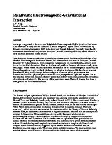
FIG. 1. Normalized energy density w ⬘ ⫽w M ⫹w A ; R ⬘ ⫽R/␭; z ⬘ ⫽z/␭; ⍀⫽2 ␲ ; j⫽s⫽2.

dependence of S N⬘ and S A⬘ on R at the plane z⫽0, are presented in Ref. 关7兴. However, to gain a better insight into the unique properties of these beams, an analysis of the spatial distributions of energy density and energy fluxes is needed. To illustrate the spatial distribution of the normalized energy density w ⬘ ⫽w M ⫹w A , it is sufficient to calculate values of w ⬘ in a meridional plane. High energy density in a very small core region 共see Fig. 1兲 is a distinguishing feature of the fields under consideration. For the beams defined by the zonal spherical harmonics (s⫽0), S A⬘ ⬅0 关7兴. Lines of energy flux for such beams lie in meridional planes 共see Figs. 2 and 3兲. For the beams with s ⫽0, lines of energy flux have twisting and spiral forms 共see Fig. 4兲. Such localized fields can be described as a kind of electromagnetic ‘‘tornados.’’

FIG. 2. Poynting’s vector field in the plane x 2 ⫽0; ⍀⫽2 ␲ ; j ⫽2, s⫽0; x ⬘ ⫽x 1 /␭; z ⬘ ⫽x 3 /␭.

FIG. 3. Poynting’s vector field with whirl structure; the parameters of the beam and the notations are the same as for Fig. 2. B. Beams with ⍀Ï2 ␲ and ␬ 0 Ï1Õ2

The beam base used above results in two different sets of orthonormal beams defined by the spherical harmonics Y sj with even and odd j, respectively. But it may be advantageous to obtain a complete system of orthonormal beams Wsj , defined by the whole set of spherical harmonics Y sj , for

which 具 Wsj 兩 Q 兩 W j ⬘⬘ 典 ⫽0 if at least one of the three conditions is met: j ⬘ ⫽ j, s ⬘ ⫽s, or the beams have the alternative polarization states (E M and E A beams兲. s

FIG. 4. Lines of energy flux; ⍀⫽2 ␲ ; j⫽s⫽2; x ⬘ ⫽x 1 /␭; y ⬘ ⫽x 2 /␭; z ⬘ ⫽x 3 /␭.

036606-4

LOCALIZED ELECTROMAGNETIC AND WEAK . . .

PHYSICAL REVIEW E 63 036606

FIG. 5. Normalized energy density w ⬘ ⫽w M ⫹w A ; R ⬘ ⫽R/␭; z ⬘ ⫽z/␭; ⍀⫽2 ␲ ; ␬ 0 ⫽1/2; j⫽2, s⫽0.

To this end, let us set the beam base by Eqs. 共2.12兲–共2.16兲 with ␪ 1 ⫽0, ␪ 2 ⫽ ␲ , and ␬ 0 ⭐ 21 . In this case, the beam manifold is the unit sphere (B⫽S 2 ), ⍀⫽2 ␲ (1⫺cos ␬0␲)⭐2␲, and

␯共 ␪ 兲⫽

2 ␭

冑

2 ␲ ␬ 0 N Q sin共 ␬ 0 ␪ 兲 . c sin ␪

共3.4兲

The smaller ␬ 0 is, the smaller is ⍀, i.e., the beam becomes more collimated. Conversely, if ␬ 0 ⫽1/2, i.e., ⍀ ⫽2 ␲ , the beam has a pronounced core region 共see Fig. 5兲. When s⫽0 and ␬ 0 ⫽ 21 , or ␬ 0 ⬇ 21 , such beams also resemble electromagnetic tornados with spiral energy fluxes. IV. ELECTROMAGNETIC STORMS, WHIRLS, AND TORNADOS

Let us briefly outline unique properties of time-harmonic localized fields Wsj 关Eq. 共2.7兲兴 with ␪ 1 ⫽0, ␲ /2⭐ ␪ 2 ⭐ ␲ , and ␬ 0 ⫽1, i.e., with ␪ ⬘ ⫽ ␪ and 2 ␲ ⭐⍀⭐4 ␲ . For the sake of simplicity, we assume that the beam state function ␯ ⫽ ␯ ( ␪ , ␸ ) reduces to a constant. A set of these exact timeharmonic solutions of the free-space homogeneous Maxwell equations consists of three subsets—‘‘storms,’’ ‘‘whirls,’’ and ‘‘tornados’’—for which time average energy flux is identically zero at all points, azimuthal and spiral, respectively. If ␪ 2 ⫽ ␲ , B⫽S 2 , and ⍀⫽4 ␲ , the fields under consideration are formed from plane waves of all possible propagation directions. They are in effect three-dimensional standing waves with a rather involved structure of interrelated electric and magnetic fields 关6–9兴. For E A and B A electromagnetic storms, both of which are defined by the zonal spherical harmonics (s⫽0), the time average Poynting vector S is vanishing at all points 关6–9兴. The electric field E of E A storms has the only nonvanishing component 共azimuthal兲, whereas the azimuthal component of the magnetic field B is everywhere zero. The opposite situation occurs with B A storms. The spherical harmonics with s⫽0 define electromagnetic

FIG. 6. Line of energy flux; ␪ 2 ⫽5 ␲ /6; j⫽4, s⫽2; x ⬘ ⫽x 1 /␭; y ⬘ ⫽x 2 /␭; z ⬘ ⫽x 3 /␭.

whirls for which the time average Poynting vector S has the only nonvanishing component 共azimuthal兲, i.e., S⫽S 0 S A⬘ eA 关6–9兴. This component, as well as the energy densities w e and w m of the electric and magnetic fields, is independent of the azimuthal angle ␺ . The whirls with j⬎s⭓1 have two major domains 共above and below the equatorial plane兲 with large energy fluxes 关8兴. The whirls with j⫽s⭓1 have only one such domain, and the energy flux peaks in the equatorial plane. Let us now consider a family of fields Wsj 关Eq. 共2.7兲兴 with ␪ 1 ⫽0, ␲ /2⬍ ␪ 2 ⬍ ␲ , and ␬ 0 ⫽1, i.e., with ␪ ⬘ ⫽ ␪ and 2 ␲ ⬍⍀⬍4 ␲ . Similar to storms and whirls, these fields are highly localized. However, the normal and radial components of time average Poynting’s vector S are not vanishing. As a result, lines of energy flux become spiral 共see Fig. 6兲, provided that s⫽0. Figure 6 shows a typical energy flux line of such a field. We refer to these unique localized fields with spiral energy flux lines as electromagnetic tornados. They bear some similarities to the fields treated in Sec. III A, but their lines of energy flux more closely resemble spirals. As ␪ 2 tends to ␲ , the step of these spirals decreases. For the fields with s⫽0, ␪ 1 ⫽0, ␲ /2⬍ ␪ 2 ⬍ ␲ , and ␬ 0 ⫽1, the lines of energy flux lie in meridional planes. These fields are intermediate in properties between the electromagnetic storms and the beams with s⫽0 and ⍀⫽2 ␲ 共see Sec. III A兲. V. LOCALIZED WEAK GRAVITATIONAL FIELDS

Electromagnetic and weak gravitational plane waves are described by antisymmetric F and symmetric h four-

036606-5

G. N. BORZDOV

PHYSICAL REVIEW E 63 036606

dimensional field tensors, respectively. Both tensors have zero trace. For each family of electromagnetic fields treated in the previous sections, there exists a similar family of weak gravitational fields defined by the same spherical harmonics. Some significant features, such as the localization of field oscillations, are characteristic for both fields. In this section, we present two types of localized weak gravitational fields in the source free space, defined by Eqs. 共2.7兲, 共2.18兲, and 共2.19兲 with ␬ 0 ⫽1 ( ␪ ⬘ ⫽ ␪ ). A. Orthonormal gravitational beams with ⍀Ä2 ␲

To obtain orthonormal gravitational beams with ⍀⫽2 ␲ , we set ␪ 1 ⫽0, ␪ 2 ⫽ ␲ /2, ␬ 0 ⫽1, and replace W( ␪ , ␸ ) 关Eq. 共2.7兲兴 by h ⫾ ( ␪ , ␸ ) 关Eq. 共2.19兲兴. In this case, the function ␯ 关Eq. 共2.6兲兴 reduces to a constant, and the beams are defined by the real parts of complex tensor functions h ⫾ 共 x兲 ⫽h ⫾ 共 r,t 兲 ⫽ ␯ 4e

⫺i ␻ t

冕 ␸冕 2␲

␲ /2

d

0

e

ikr•er ( ␪ , ␸ )

0

FIG. 7. Normalized intensity w ⬘ of metric oscillations w ⬘ ⫽2w ⫺ / ␯ 24 ; R ⬘ ⫽R/␭; z ⬘ ⫽z/␭; ⍀⫽2 ␲ ; j⫽3; s⫽2. † w ⫾⫽共 h ⫾ h⫾兲t

Y sj 共 ␪ , ␸ 兲

⫽

⫻h ⫾ 共 ␪ , ␸ 兲 sin ␪ d ␪

⫺ ␳ 2 I ss⫺1 关 sin ⴰ2⫾2 j

1

兺

p⫽0

2 2 兵 共 J ss⫺2 j p 关 1⫹cos ⫾2 cos兴 兲

ss⫺1 2 2 2 ⫹ 共 J ss⫹2 j p 关 1⫹cos ⫿2 cos兴 兲 ⫹ 共 J j p 关 sin ⴰ2⫾2 sin兴 兲

␯4 ⫽ e i(s ␺ ⫺ ␻ t) 兵 ␳ I ss⫺2 关 1⫹cos2 ⫾2 cos兴 j 2 ⫹ ␳ * I ss⫹2 关 1⫹cos2 ⫿2 j

␯ 24 16

ss 2 2 2 ⫹ 共 J ss⫹1 j p 关 sin ⴰ2⫿2 sin兴 兲 ⫹6 共 J j p 关 sin 兴 兲 其 .

cos兴

共5.5兲

Naturally, the normalization constant N Q 关Eq. 共2.3兲兴 must satisfy the condition w ⫾ Ⰶ1. Then we obtain

sin兴

2 ⫺ ␳ 2* I ss⫹1 关 sin ⴰ2⫿2 sin兴 ⫹ 共 ␳ 3 ⫺ ␳ 1 兲 I ss j j 关 sin 兴 其 ,

具 h ⫾兩 Q ⫾兩 h ⫾典 ⫽

共5.1兲

冕

␴0

† Q ⫾ h ⫾ 兲 t d ␴ 0 ⫽N Q , 共h⫾

共5.6兲

where the integrand is given by

where

␳ ⫽e 丢 e,

␳ 1 ⫽e 丢 e* ⫹e* 丢 e⫽ 21 共 1⫺ ␳ 3 兲 ,

␳ 2 ⫽ 12 共 e 丢 e3 ⫹e3 丢 e兲 , e⫽ 共 eR ⫹ieA 兲 /2,

␳ 3 ⫽e3 丢 e3 ,

␯ 4⫽

1 冑2N Q . ␭

共5.2a兲

␯ 24 † Q ⫾ h ⫾ 兲 t ⫽⫾ 共h⫾ 8

1

兺

p⫽0

2 2 兵 共 J ss⫺2 j p 关 1⫹cos ⫾2 cos兴 兲

1 ss⫺1 2 2 ⫺ 共 J ss⫹2 j p 关 1⫹cos ⫿2 cos兴 兲 ⫹ 2 共 J j p 关 sin ⴰ2

共5.2b兲

2 ⫾2 sin兴 兲 2 ⫺ 21 共 J ss⫹1 j p 关 sin ⴰ2⫿2 sin兴 兲 其 . 共5.7兲

共5.3兲

If s⫽0, the latter reduces to 1

sm Complex scalar functions I sm j 关 f 兴 ⫽I j 关 f 兴 (r, ␥ ) are defined s by the spherical harmonics Y j , an integer m, and a scalar function f ⫽ f ( ␪ ). The definitions and the properties of these functions are presented in Ref. 关7兴. The above notations emphasize the fact that I sm j 关 f 兴 (r, ␥ ) at fixed r and ␥ are functionals regarding f. For any given f, I sm j 关 f 兴 (r, ␥ ) is a function of r and ␥ . When it will not cause a misunderstanding, we omit the arguments (r, ␥ ) and/or 关 f 兴 . The real and imaginary parts of I sm j can be separated as 关7兴 兩 m 兩 sm I sm 共 J j0 ⫹iJ sm j ⫽i j1 兲 .

† Q ⫾ h ⫾ 兲 t ⫽ ␯ 24 共h⫾

02 2 兵 J 02 j p 关 cos兴 J j p 关 1⫹cos 兴

01 ⫹ 12 J 01 j p 关 sin兴 J j p 关 sin ⴰ2 兴 其 ,

共5.8兲

and w ⫹ ⫽w ⫺ . For the beams h ⫺ and h ⫹ , defined by the spherical harmonic Y 23 , the intensity of metric oscillations is illustrated in Figs. 7 and 8. Orthonormal gravitational beams with ⍀⭐2 ␲ and ␬ 0 ⭐ 12 can be obtained by using a beam state function that differs from ␯ ( ␪ ) 关Eq. 共3.4兲兴 only by a constant factor.

共5.4兲

The intensity of metric oscillations is characterized by the norm w⫽(hh † ) t . Hence, we obtain

兺

p⫽0

B. Gravitational whirls and storms

Let us now set ␪ 1 ⫽0, ␪ 2 ⫽ ␲ , ␬ 0 ⫽1, and define the amplitude function by Eqs. 共2.18兲, assuming that the beam state

036606-6

LOCALIZED ELECTROMAGNETIC AND WEAK . . .

PHYSICAL REVIEW E 63 036606

FIG. 8. Normalized intensity w ⬘ of metric oscillations w ⬘ ⫽2w ⫹ / ␯ 24 ; R ⬘ ⫽R/␭; z ⬘ ⫽z/␭; ⍀⫽2 ␲ ; j⫽3; s⫽2.

FIG. 9. Normalized intensity w ⬘ of metric oscillations w ⬘ ⫽2w 1 / ␯ 24 ; R ⬘ ⫽R/␭; z ⬘ ⫽z/␭; ⍀⫽4 ␲ ; j⫽3; s⫽1.

function ␯ reduces to a constant. This results in two sets of weak gravitational fields that are defined by the real parts of the complex tensor functions

w 1⫽

h n 共 x兲 ⬅h n 共 r,t 兲 ⫽ ␯ 4 e ⫺i ␻ t

冕 ␸冕 2␲

␲

d

0

␯ 24 ss⫹2 2 2 2 2 兵 共 J ss⫺2 j p 关 1⫹cos 兴 兲 ⫹ 共 J j p 关 1⫹cos 兴 兲 4 ss⫹1 ss 2 2 2 2 ⫹ 共 J ss⫺1 jq 关 sin ⴰ2 兴 兲 ⫹ 共 J jq 关 sin ⴰ2 兴 兲 ⫹6 共 J j p 关 sin 兴 兲 其 ,

e ikr•er ( ␪ , ␸ )

共5.12a兲

0

⫻Y sj 共 ␪ , ␸ 兲 h n 共 ␪ , ␸ 兲 sin ␪ d ␪ ,

ss⫹2 2 2 w 2 ⫽ ␯ 24 兵 共 J ss⫺2 jq 关 cos兴 兲 ⫹ 共 J jq 关 cos兴 兲

共5.9兲

where n⫽1,2, and the scalar coefficient ␯ 4 specifies the amplitudes of partial plane waves ( ␯ 4 Ⰶ1). Substitution of h 1 and h 2 关Eq. 共2.18兲兴 in Eq. 共5.9兲 yields 2 h 1 ⫽ ␯ 4 i 兩 s 兩 ⫹p e i(s ␺ ⫺ ␻ t) 兵 ␳ ␣ 共 s 兲 J ss⫺2 j p 关 1⫹cos 兴

ss⫹1 2 2 ⫹ 共 J ss⫺1 j p 关 sin兴 兲 ⫹ 共 J j p 关 sin兴 兲 其 .

Figures 9 and 10 illustrate the intensity of the metric oscillations in the core regions of the whirls h 1 and h 2 , defined by the spherical harmonic Y 13 . Gravitational storms are defined by the zonal spherical harmonics as

2 q ⫹ ␳ * ␣ 共 ⫺s 兲 J ss⫹2 j p 关 1⫹cos 兴 ⫺ ␳ 2 共 ⫺1 兲 ␤ 共 ⫺s 兲

h 1⫽

* 共 ⫺1 兲 q ␤ 共 s 兲 J ss⫹1 ⫻J ss⫺1 jq 关 sin ⴰ2 兴 ⫺ ␳ 2 jq 关 sin ⴰ2 兴 2 ⫹ 共 ␳ 3 ⫺ ␳ 1 兲 J ss j p 关 sin 兴 其 ,

共5.12b兲

共5.10a兲

␯ 4 p ⫺i ␻ t 2 i e 兵 共 eA 丢 eA ⫺eR 丢 eR 兲 J 02 j p 关 1⫹cos 兴 2 ⫺ 共 eR 丢 e3 ⫹e3 丢 eR 兲共 ⫺1 兲 q J 01 jq 关 sin ⴰ2 兴 2 ⫹2 共 ␳ 3 ⫺ ␳ 1 兲 J 00 j p 关 sin 兴 其 ,

h 2 ⫽2 ␯ 4 i 兩 s 兩 ⫹p e i(s ␺ ⫺ ␻ t) 兵 ␳ ␣ 共 s 兲共 ⫺1 兲 p J ss⫺2 jq 关 cos兴

共5.13a兲

⫺ ␳ * ␣ 共 ⫺s 兲共 ⫺1 兲 p J ss⫹2 jq 关 cos兴 ss⫹1 ⫺ ␳ 2 ␤ 共 ⫺s 兲 J ss⫺1 j p 关 sin兴 ⫹ ␳ * 2 ␤ 共 s 兲 J j p 关 sin兴 其 ,

共5.10b兲 where

␤共 s 兲⫽

再

⫺1

共 s⫽⫺1,⫺2, . . . 兲

1

共 s⫽0,1,2, . . . 兲 ,

共5.11兲

␣ (s)⫽2 ␦ 1s ⫺1, p⫽1⫺q⫽0 if j⫹ 兩 s 兩 is even, and p⫽1 ⫺q⫽1 if j⫹ 兩 s 兩 is odd. The traces and the four-dimensional determinants of these tensors are vanishing at all points, and e4 •h n ⫽h n •e4 ⬅0, n⫽1,2. The intensities of metric oscillations for these fields are given by

FIG. 10. Normalized intensity w ⬘ of metric oscillations w ⬘ ⫽2w 2 / ␯ 24 ; R ⬘ ⫽R/␭; z ⬘ ⫽z/␭; ⍀⫽4 ␲ ; j⫽3; s⫽1.

036606-7

G. N. BORZDOV

PHYSICAL REVIEW E 63 036606

FIG. 11. Normalized instantaneous energy density w ⬘ of an electromagnetic whirl moving with the velocity V⫽0.4 c e1 ⬘ with respect to the frame L ⬘ ; j⫽4; s⫽2; x ⬘ ⫽x 1 ⬘ /␭; y ⬘ ⫽x 2 ⬘ /␭; x 3 ⬘ ⫽0.

h 2 ⫽ ␯ 4 i ⫺q e ⫺i ␻ t 兵 共 eR 丢 eA ⫹eA 丢 eR 兲共 ⫺1 兲 p J 02 jq 关 cos兴 ⫹ 共 eA 丢 e3 ⫹e3 丢 eA 兲 J 01 j p 关 sin兴 其 .

共5.13b兲

VI. MOVING AND EVOLVING STORMS, WHIRLS, AND TORNADOS

The localized electromagnetic and gravitational fields discussed above are time-harmonic in the Lorentz reference frame L with basis (ei ). In any other Lorentz frame L ⬘ with basis (e⬘i ), they will be observed as a kind of electromagnetic 关7兴 or gravitational missile moving without dispersing at speed V⬍c. Because of the very involved dependence of complex fields E, B, or h on time and spatial coordinates, parameters 兩 E兩 2 , 兩 B兩 2 , or w⫽(hh † ) t provide only a rough idea of the missile field structure 关7兴, whereas instantaneous values of real fields give an accurate picture. Figures 11 and 12 illustrate both the localization of field oscillations and the asymmetry 共Fig. 11兲 caused by the movement of whirls. The time-harmonic solutions presented in the previous sections can be applied as reasonably accurate models of real physical fields. A more realistic description can be achieved by integrating these solutions with respect to frequency 关7兴. As illustration, let us consider basic properties of quasimonochromatic fields defined by Eqs. 共2.21兲 and 共2.22兲. To be specific, we discuss below evolving electromagnetic whirls, but other evolving electromagnetic and weak gravitational fields 共storms and tornados兲 can be treated similarly. ˘ sj (r,t) 关Eq. 共2.22兲兴 is formed from the infiniThe field W tesimal plane-wave packets with the envelope function j 0共 p 0␸ 0 兲 ⫽

sin共 p 0 ␸ 0 兲 , p 0␸ 0

FIG. 12. Normalized instantaneous energy density w ⬘ of an electromagnetic whirl moving with the velocity V⫽0.4 c e1 ⬘ with respect to the frame L ⬘ ; j⫽4; s⫽2; x ⬘ ⫽x 1 ⬘ /␭; z ⬘ ⫽x 3 ⬘ /␭; x 2 ⬘ ⫽0.

r⫽0. At t⫽0, the whirl reaches its maximum intensity and closely resembles a time-harmonic whirl. In particular, lines of energy flux are circular for both whirls. At ⫺ ␲ /⌬ ␻ ⬍t ⬍0 and 0⬍t⬍ ␲ /⌬ ␻ , the energy flux lines of the evolving whirl are convergent 共Fig. 13兲 and divergent 共Fig. 14兲, respectively. When t→⫾⬁, the field tends to zero at all points r.

共6.1兲

where ␸ 0 ⫽r•k( ␪ , ␸ )⫺ ␻ t. Since p 0 Ⰶ1, the field can be described as an evolving whirl in the neighborhood of the point

FIG. 13. Convergent lines of energy flux of an evolving electromagnetic whirl; ⍀⫽4 ␲ ; j⫽s⫽4; p⫽0.05; ct⫽⫺7␭; x ⬘ ⫽x 1 /␭; y ⬘ ⫽x 2 /␭; z ⬘ ⫽x 3 /␭.

036606-8

LOCALIZED ELECTROMAGNETIC AND WEAK . . .

PHYSICAL REVIEW E 63 036606

FIG. 15. Radial component S R⬘ of the normalized energy flux vector as a function of R ⬘ ⫽R/␭ ; z⫽0; j⫽s⫽4; ⌬ ␻ / ␻ ⫽0.05; (A) ct⫽⫺40␭; (B) ct⫽30␭.

FIG. 14. Divergent lines of energy flux of an evolving electromagnetic whirl; ⍀⫽4 ␲ ; j⫽s⫽4; p⫽0.05; ct⫽8␭; x ⬘ ⫽x 1 ⬘ /␭; y ⬘ ⫽x 1 ⬘ /␭; z ⬘ ⫽x 3 ⬘ /␭.

The evolution of the field can be described as follows. A whirl originates at infinity at t⫽⫺⬁ as an infinitely small converging wave. At tⰆ⫺ ␲ /⌬ ␻ , there is a very small converging wave with a maximum peak at the distance r ⫽⫺ct 共see curve A in Fig. 15兲. During all this time, there is also a weak whirl in the neighborhood of the point r⫽0. It passes through maxima and minima of activity, gradually gaining in intensity as t→0. Figure 15 illustrates the radial energy fluxes at two different instants of minimum whirl activity. The total field can be described as the superposition of converging and expanding waves with ever-changing proportion. At t⬎0, the whirl, still passing through maxima and minima of activity, gradually transforms into an expanding wave 共see curve B in Fig. 15兲, which vanishes in infinity as t→⫹⬁. It follows from Eq. 共2.23兲 that the evolving storms, whirls, and tornados have finite total energy. VII. CONCLUSION

Unique solutions of wave equations, which describe localized electromagnetic and weak gravitational time-harmonic fields in the source-free space, are obtained using expansions in plane waves. These fields have a very small and clearly defined core region with maximum intensity of field oscillations. Outside the core, the intensity of oscillations rapidly decreases in all directions. Each family of solutions consists of vector or tensor functions that have integral expansions in plane waves propagating in the same given solid angle ⍀. Our main concern in this paper is with the families of orthonormal beams with ⍀⫽2 ␲ and the families of threedimensional standing waves with ⍀⫽4 ␲ . In addition, some

specific electromagnetic fields with ⍀⭐2 ␲ and 2 ␲ ⭐⍀ ⭐4 ␲ are presented. The peculiarities of energy transport in such fields are illustrated by the example of localized electromagnetic fields. In a given Lorentz frame L, a set of the obtained exact time-harmonic solutions of the free-space homogeneous Maxwell equations consists of three subsets 共storms, whirls, and tornados兲 for which time average energy flux is identically zero at all points, azimuthal and spiral, respectively. In any other Lorentz frame L ⬘ , they will be observed as a kind of electromagnetic missile moving without dispersing at speed V⬍c. The properties of evolving fields, obtained by integrating the time-harmonic solutions with respect to frequency, are briefly outlined. Since evolving electromagnetic storms, whirls, tornados, and various types of moving and evolving missiles are described by the exact solutions of Maxwell’s equations and have finite total energy, they may exist in nature or can be excited. To this end, the modern antenna technology 关19兴 provides promising tools, such as large array antennas with tens of thousands and even well over 100 000 elements, active integrated antennas, and beam-forming techniques. In this paper, the localized gravitational fields are treated in the linear approximation. This gives grounds to propose the problem of searching for exact solutions of the Einstein empty space field equations, which reduce, in the case of weak fields, to the solutions presented above. In solving this problem, the evolving weak fields can be used as the initial conditions. To this end, it is necessary to set the initial moment t 0 Ⰶ⫺ ␲ /⌬ ␻ and the parameter N Q in such a way as to obtain a weak converging wave at t⭐t 0 . If N Q is sufficiently small, the evolving field will remain everywhere weak at any t⬎t 0 . However, by decreasing t 0 and increasing N Q , one can set the initial conditions to search for a nonlinear evolving field that is everywhere weak and can be described by the presented solutions only at t⭐t 0 . The further evolution of this converging wave should be investigated by solving the Einstein equations.

036606-9

G. N. BORZDOV 关1兴 关2兴 关3兴 关4兴 关5兴 关6兴

关7兴 关8兴

关9兴

关10兴 关11兴

PHYSICAL REVIEW E 63 036606

J.N. Brittingham, J. Appl. Phys. 54, 1179 共1983兲. R.W. Ziolkowski, J. Math. Phys. 26, 861 共1985兲. A. Sezginer, J. Appl. Phys. 57, 678 共1985兲. T.T. Wu and R.W.P. King, J. Appl. Phys. 56, 2587 共1984兲. T.T. Wu, J. Appl. Phys. 57, 2370 共1985兲. G.N. Borzdov, in 7th International Symposium on Recent Advances in Microwave Technology Proceedings, Ma´laga, 1999, ˜ alosa and B.S. Rawat 共CEDMA, edited by C. Camacho Pen Ma´laga, 1999兲, pp. 169–172. G.N. Borzdov, Phys. Rev. E 61, 4462 共2000兲. G.N. Borzdov, in ESA SP-444 Proceedings of the Millennium Conference on Antennas & Propagation AP2000, Davos, 2000 共ESA, ESTEC, Noordwijk, 2000兲, p0131.pdf; in ibid., p0132.pdf. G.N. Borzdov, in Proceedings of Bianisotropics 2000: 8th International Conference on Electromagnetics of Complex Media, Lisbon, 2000, edited by A.M. Barbosa and A.L. Topa ˜ es, Lisbon, 2000兲, pp. 11–14; in 共Instituto de Telecomucaco ibid., pp. 55–58; in ibid., pp. 59–62. G.N. Borzdov, Opt. Commun. 94, 159 共1992兲; J. Math. Phys. 34, 3162 共1993兲. G.N. Borzdov, in Advances in Complex Electromagnetic Materials, edited by A. Priou, A. Sihvola, S. Tretyakov, and A. Vinogradov 共Kluwer, Dordrecht, 1997兲, pp. 71–84.

关12兴 G.N. Borzdov, in Proceedings of Bianisotropics’98: 7th International Conference on Complex Media, Braunschweig, 1998, edited by A.F. Jacob and J. Reinert 共Technische Universita¨t Braunschweig, Braunschweig, 1998兲, pp. 261–264; in ibid., pp. 301–304. 关13兴 G.N. Borzdov, in Proceedings of Progress in Electromagnetics Research Symposium, Nantes, 1998 共IRESTE–Universite´ de Nantes, Nantes, 1998兲, p. 516. 关14兴 G.N. Borzdov, in Electromagnetic Fields in Unconventional Materials and Structures, edited by O.N. Singh and A. Lakhtakia 共Wiley Interscience, New York, 2000兲, pp. 83–124. 关15兴 G.N. Borzdov, J. Math. Phys. 38, 6328 共1997兲. 关16兴 L.C. Biedenharn and J.D. Louck, Angular Momentum in Quantum Physics 共Addison-Wesley, Reading, MA, 1981兲. 关17兴 E.T. Whittaker and G.N. Watson, A Course of Modern Analysis 共Cambridge University Press, Cambridge, 1927兲. 关18兴 L.D. Landau and E.M. Lipshitz, Field Theory 共Nauka, Moscow, 1973兲. 关19兴 E. Brookner, in ESA SP-444 Proceedings of the Millennium Conference on Antennas & Propagation AP2000, Davos, 2000 共ESA, ESTEC, Noordwijk, 2000兲, p1487.pdf; P. Hall, in ibid., p0221.pdf; R. Mailloux, in ibid., p1549.pdf; E. Magill, in ibid., p0426.pdf.

036606-10