Geoinformatica DOI 10.1007/s10707-007-0022-3
Logical Representation of a Conceptual Model for Spatial Data Warehouses Elzbieta Malinowski · Esteban Zimányi
Received: 12 May 2006 / Accepted: 9 January 2007 © Springer Science + Business Media, LLC 2007
Abstract The MultiDimER model is a conceptual model used for representing a multidimensional view of data for Data Warehouse (DW) and On-Line Analytical Processing (OLAP) applications. This model includes a spatial extension allowing spatiality in levels, hierarchies, fact relationships, and measures. In this way decisionmaking users can represent in an abstract manner their analysis needs without considering complex implementation issues and spatial OLAP tools developers can have a common vision for representing spatial data in a multidimensional model. In this paper we propose the transformation of a conceptual schema based on the MultiDimER constructs to an object-relational schema. We based our mapping on the SQL:2003 and SQL/MM standards giving examples of commercial implementation using Oracle 10g with its spatial extension. Further we use spatial integrity constraints to ensure the semantic equivalence of the conceptual and logical schemas. We also show some examples of Oracle spatial functions, including aggregation functions required for the manipulation of spatial data. The described mappings to the object-relational model along with the examples using a commercial system show the feasibility of implementing spatial DWs in current commercial DBMSs. Further, using integrated architectures, where spatial and thematic data is defined within the same DBMS, facilitates the system management simplifying data definition and manipulation.
The work of E. Malinowski was funded by a scholarship of the Cooperation Department of the Université Libre de Bruxelles. Currently on leave from the Universidad de Costa Rica. E. Malinowski (B) · E. Zimányi Department of Informatics & Networks, Université Libre de Bruxelles, 50 av. F.D. Roosevelt, 1050 Brussels, Belgium e-mail:
[email protected] E. Zimányi e-mail:
[email protected]
Geoinformatica
Keywords spatial data warehouses · spatial databases · logical modeling · spatial hierarchies · spatial measures 1 Introduction Data Warehouses (DWs) store and provide access to large volumes of historical data supporting the strategic decisions of organizations. The structure of DWs is based on a multidimensional view of data usually represented as a star or a snowflake schema, consisting of fact and dimension tables. A fact table contains numeric data called measures (e.g., Sales, Cost). Dimensions contains attributes that allow to explore measures from different perspectives. These attributes can either form a hierarchy (e.g., Product–Category–Department) or be descriptive (e.g., Product description). On-Line Analytical Processing (OLAP) systems allow dynamic manipulations of data contained in DWs. In particular, hierarchies allow the user to start from a general view of data and obtain a detailed view with the drill-down operation. Alternatively, the roll-up operation allows to transform detailed measures into summarized data. Since it is estimated that about 80% of data stored in databases has a spatial or location component [28], location dimensions have been widely integrated in DWs and in OLAP systems. However, these dimensions are usually represented in an alphanumeric, non-cartographic manner, since these systems are neither able to store nor to manipulate spatial data. The management of this kind of data is usually carried out by Spatial Databases (SDBs) or Geographic Information Systems (GISs). Spatial Data Warehouses (SDWs) combine data warehouse and spatial database technologies. SDWs keep the intrinsic concepts of a DW and additionally provide support to store, index, aggregate and analyze spatial data [6]. SDWs raise several issues, in particular, storage and indexing structures, aggregation of spatial data, visualization, etc. Nevertheless, very little attention from the research community has been drawn to conceptual modeling for SDWs and its subsequent mapping into a logical model. Extending a multidimensional model by the inclusion of spatial data provides a concise and organized SDW representation [1]. It facilitates the delivery of data for spatial OLAP (SOLAP) systems, spatial data mining, and spatial statistical analysis. Further, since it is platform independent, a conceptual multidimensional model allows to establish a communication bridge between users and designers. It reduces the difficulties of modeling spatial applications, since decision-making users do not usually possess the expertise required by software currently used for managing spatial data. Although both SDBs and SDWs manage spatial data, their purpose is different. SDBs are used for answering queries that involve spatial location, e.g., where is the closest store to my house, which highways connect Brussels and Warsaw, how to get to a specific place from my current position given by a GPS. In contrast, SDWs use only the data of SDBs that is needed to support the decision-making process, e.g., what is the best location for a new store, which alternative routes can be built for highways with intensive traffic. As a consequence, even though there are proposals of conceptual models for SDBs, we believe that they are not adequate for SDWs: a spatial multidimensional model can better express the requirements of decisionmaking users.
Geoinformatica
Therefore, in [15] and [17] we proposed a conceptual model, the MultiDimER model, that allows to produce conceptual schemas based on a multidimensional view of data with different kinds of spatial hierarchies, spatial fact relationships, and spatial measures. Our model is mainly based on the ER constructs (i.e., entity types, relationship types, attributes) with their usual semantics. Some additional semantics is provided for different kinds of (spatial) hierarchies ([14], [17]) that is beyond the scope of this paper. In this work we propose the mapping of a MultiDimER schema to a logical schema based on an object-relational (OR) approach. The proposed mapping to an OR representation is based on well-known rules for mapping from the ER model to the relational model, e.g., [4]. Further, since in the translation process from a conceptual schema to a logical schema some semantics may be lost, we give examples of the integrity constraints implemented in Oracle 10g that allow to preserve this semantics. We also show some examples of using spatial operators and spatial aggregations functions in SDW applications. In our approach we have chosen an integrated architecture based on spatial extensions of current object-relational DBMSs. This integrated architecture allows to represent spatial and non-spatial data in the same system instead of relying on proprietary GIS solutions where different kinds of data are managed separately. Integrated architecture simplifies modeling, use, integration, and querying of spatial and non-spatial data. Further, spatial extensions in DBMSs are mostly based on existing standards such as the SQL:2003 [18] and SQL/MM [11] standards. The former specifies features of an object-relational representation that allow to manage complex data. The latter includes the specification for spatial data and functions. We have chosen Oracle 10g as an example of a DBMS, since it contains many of the features specified by above mentioned standards and since it also includes spatial aggregation functions, which are not specified in the SQL/MM standard, but are required in managing multidimensional data. Further, using a commercially-available DBMS, we show the applicability of the proposed solutions in real-world situations. Moreover, a logical model for spatial data can use structures that allow to store in a persistent way the topological relationships existing between spatial objects. These kinds of models are called topological or network depending on whether planar or linear spatial objects are represented [27]. Another option is to store the geometry of each object and compute topology “on the fly” when it is required. This model is called the spaghetti model. We have chosen the spaghetti model due to the intrinsic semantics of multidimensional models. In this paper, Section 2 briefly presents the main features of the MultiDimER model. Section 3 motivates our approach for an integrated architecture based on an object-relational model with a spatial extension. Section 4 to 6 present the mappings of spatial levels, spatial hierarchies, and spatial fact relationships, respectively. Finally, related works are surveyed in Section 7 and Section 8 concludes our paper.
2 Overview of the MultiDimER model In this section we briefly recall the definition of the spatially-extended MultiDimER model presented in [15]. A schema is defined as a finite set of dimensions and fact relationships. A dimension is an abstract concept for grouping data that shares a
Geoinformatica
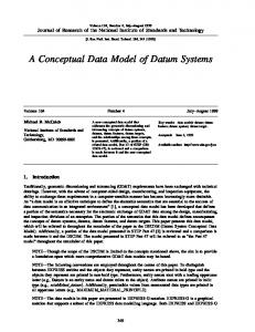
common semantic meaning within the domain being modeled. It represents either a level, or one or more hierarchies. Levels correspond to entity types (Fig. 1a). An instance of a level is called a member. Hierarchies are required for establishing meaningful paths for the roll-up and drill-down operations. A hierarchy contains several related levels (Fig. 1b). Given two consecutive levels of a hierarchy, the higher level is called parent and the lower level is called child. A level that does not have a child level is called leaf ; the last level, i.e., the one does not have a parent level, is called root. Cardinalities (Fig. 1c) indicate the minimum and maximum number of members in one level that can be related to a member in another level. Hierarchies can express different structures according to an analysis criterion (Fig. 1d), e.g., geographical location, organizational structure, etc. Levels have one or several key attributes (represented in bold and italic in Fig. 1) and may also have other descriptive attributes. Key attributes of a parent level define how child members can be grouped. Key attributes in a leaf level or in a level forming a dimension without hierarchy indicate the granularity of measures in the associated fact relationship. We define a spatial level as a level for which the application needs to keep its spatial characteristics. This is captured by its geometry, which is represented using spatial data types such as point, line, surface, or a collection of these data types. Such geometry is expressed in a spatial reference system. Further, two consecutive spatial levels forming a hierarchy relate to each other with topological relationships existing between their spatial components, such as contains, equals, intersects, overlaps, etc. [3]. By default we suppose the contains topological relationship, i.e., the geometry of a parent member contains the geometries of its child members. We use the pictograms of the MADS model [21] for representing the geometry of spatial levels (Fig. 1e) as well as topological relationships between them (Fig. 1f).
Level
Level2
Level1
Key attribute Other attributes
Key attribute Other attributes
Key attribute Other attributes a)
b) (1, N) (0,N) c)
(1,1) (0,1)
Criterion d)
Point
Point set
Intersects
Equals
Line
Line set
Contains
Touches
Surface
Surface set
Disjoint
Crosses
e)
Fact relationship
Measures g)
f)
Fig. 1 Notations for our multidimensional model: a one-level dimension, b hierarchy, c cardinalities, d analysis criterion, e geometry types, f topological relationships, and g fact relationship with associated measures
Geoinformatica Fig. 2 An example of a multidimensional schema with spatial elements
State
Highway Highway name Other attributes
Highway Section
Road Coating Coating name Coating type Coating durability Other attributes
Section number Other attributes Highway maintenance Highway Structure Highway Segment Segment number Road condition Speed limit Other attributes
State name State population State area State major activity Capital Other attributes Geo Location County County name County population County area Other attributes Time
Length (S) Common area No. cars Repair cost
Date Event Season Other attributes
We adopt an orthogonal approach where a level may have geometry independently of the fact that it has spatial attributes. This achieves maximal expressive power where, e.g., a level such as State may be spatial or not depending on application requirements, and may have (descriptive) spatial attributes such as Capital (Fig. 2). We define a spatial hierarchy as a hierarchy that includes at least one spatial level. Similarly, a spatial dimension is a dimension that includes at least one spatial hierarchy. Usual non-spatial dimensions and hierarchies are called thematic. Spatial hierarchies can combine thematic and spatial levels. A fact relationship (Fig. 1g) represents an n-ary relationship between leaf levels. A spatial fact relationship is a fact relationship that requires a spatial join between two or more spatial dimensions. Further, the spatial join can be based on different predicates represented by topological relationships, e.g., intersects. A (spatial) fact relationship may contain measures that can be spatial or thematic. The latter usually represent numerical data meaningful for leaf members that are aggregated while traversing a hierarchy. The former can be represented by geometry or calculated using spatial operators, such as distance, area, etc. To indicate that measure is calculated using spatial operators, we use the symbol (S). Measures require the specification of the function used for aggregations along the hierarchies. By default we suppose sum for the measures represented as numbers and geometric union for the measures represented as geometries. An example of a multidimensional schema with spatial elements using our notation is given in Fig. 2. It represents a schema for the analysis of highway maintenance costs. It contains two spatial dimensions, Highway Segment1 (of type Line) and County (of type Area), as well as two thematic dimensions, Road Coating and Time.
1 We
call a dimension using its leaf level name.
Geoinformatica
Both spatial dimensions contain the levels forming the hierarchies.2 Additionally the spatial level State includes a spatial descriptive attribute Capital. Since the fact relationship relates all dimensions, it represents a usual join for the thematic dimensions and an intersection topological relationship for the spatial dimensions (the latter represented in Fig. 2 with the symbol .) Additionally, the schema contains two thematic measures: No. cars and Repairing cost, and two spatial measures: Length and Common area. Length is a number representing the length of the part of a highway segment that belongs to a county while Common area is a spatial data representing the geometry of this part.
3 Motivation In this section, we present our rationale for transforming a conceptual multidimensional model into a logical model based on an object-relational representation. We also refer to the advantages of using an integrated architecture available in spatially-extended DBMSs (e.g., Oracle Spatial). Next, we express the motivation for applying the spaghetti data model to represent geometries of spatial data. Finally, we refer to the importance of preserving semantics during the transformation from conceptual into logical schemas. Using the surrogate-based object-relational model In general, logical-level implementations for SDBs can be based on relational, object-oriented, or object-relational approaches [33]. The relational model has well-known limitations for representing complex, non-atomic data. For example, since spatial features are modeled using only conventional atomic attribute types, a polygon is stored as a set of rows each having the coordinates of two points representing a line segment forming the polygon. Therefore, the relational model imposes to users the responsibility of knowing and maintaining the groupings of rows representing the same real-world object in all their interactions with the database. The object-oriented approach can solve these problems using complex objects for representing geometries. However, a pure object-oriented approach has not been yet widely integrated into current DBMSs. On the other hand, the object-relational (OR) model preserves the foundations of the relational model allowing to have a declarative access to data and extends its modeling power organizing data using an object model. The OR model allows attributes to have complex types, i.e., inherently groups related facts into a single row, e.g., a polygon can be represented in one row. In addition, OR features are also included in the SQL:2003 standard [18] and in leading DBMSs, such as Oracle or Informix. We use surrogates in our mapping instead of relying on user-defined keys for several reasons. First, DWs typically use system-generated keys for ensuring better performance during join operations and independence from transactional systems. Further, surrogates do not vary over time so that two entities having identical surrogates represent the same entity, thus allowing to include historical data in an unambiguous way. In addition, in some situations it is necessary to store the
2 For
simplicity we did not include hierarchies in the thematic dimensions.
Geoinformatica
information about an entity either before it has been assigned a user-controlled key value or after it has ceased to have one. Finally, the SQL:2003 standard and several commercial DBMSs (e.g., Oracle 10g) support surrogates. Nevertheless, the object-relational model without surrogates can also be used in our mapping, replacing the surrogates with user-defined keys independent from those used in source systems. Using spatially-extended DBMSs Two different architectures may be used for the storage and management of spatial data: dual and integrated [32]. The former is based on separate management systems for spatial and non-spatial data while the latter extends DBMSs with spatial data types (e.g., point, line, and polygon) and functions (e.g., overlap, distance, and area) [32]. A dual architecture is used by traditional GISs. It requires heterogeneous data models to represent spatial and non-spatial data. Further, spatial data is usually represented using proprietary data structures [32], which implies difficulties in modeling, use, and integration, i.e., it leads to increasing complexity of system management. On the other hand, spatially-extended DBMSs offer support for storage, retrieval, query, and updating of spatial objects while preserving other DBMS functionalities, such as recovery techniques and optimization [27]. These spatially-extended DBMSs allow users to define an attribute of a table as being of spatial type, to retrieve topological relationships between spatial objects using spatial operators, to speed up spatial queries using spatial indexes, etc. Several commercial DBMSs support the management of spatial data, e.g., Oracle Spatial, Spatial Extender of IBM’s DB/2, or PostGIS of PostgreSQL. This support in based in more or less details on existing standards [31]. For example, the OpenGIS Consortium (OGC) has defined Simple Feature Specification (SFS) for SQL [19] standardizing the basic spatial types and functions as an extension of SQL. Further, the SQL:2003 standard was extended by the ISO/IEC 13249 SQL/MM standard [11] for managing multimedia and application-specific packages. This extension includes several parts, one of which defines how to store, retrieve, and process spatial data in a relational database system. Using the spaghetti spatial data model Two different logical models can be used when storing spatial data: topological and spaghetti models [27]. The former describes geometries allowing to represent the topology in a “persistent” way, i.e., creating data structures so that the topological relationships are stored and available persistently in the database. On the other hand, the spaghetti model represents geometries of spatial objects in a way that the topology must be computed “on the fly,” i.e., when it is needed for selected subset of spatial objects [27]. We have chosen a spaghetti data model since it allows to store all spatial objects independently. Thus, it is simple and it facilitates insertion of new objects, i.e., users do not need to know a priori the topological relationships between different spatial objects. In contrast, the topological model is more complex and it has less flexibility for introducing new spatial objects [7]. It also requires much more volumes of data compared to the spaghetti model. Further, a topological model for representing hierarchies guarantees only the so-called “horizontal consistency” [7], i.e., maintaining topological relationships between members belonging to the same level. However, in DWs and OLAP
Geoinformatica
systems, hierarchies are used for traversing from one level to another and information about the topological relationships between spatial members belonging to the same level is rarely required. Even though some solutions were proposed for representing hierarchies using a topological model (e.g., [7]), i.e., representing in a persistent way the topological relationships between all members belonging to child and parent levels, they include conditions that are too restrictive for our model. For example, imposing that the geometry of every child member must be contained in the geometry of its corresponding parent member and that the geometry of every parent member must be the union of the geometries of the corresponding child members do not allow to model the different kinds of spatial hierarchies proposed in [17]. Preserving semantics Conceptual models, including the MultiDimER model, provide constructs for representing in a more direct way the semantics of the modeled reality. However, much of this semantics may be lost when translating a conceptual schema into a logical schema since only the concepts supported by the target DBMS can be used. To ensure the semantic equivalence between the conceptual and the logical schemas, integrity constraints can be introduced. The idea of having explicit integrity constraints for spatial data is not new in the spatial database community (e.g., [2], [34]). Current DBMSs provide support for declarative integrity constraints, such as keys, referential integrity, or check constraints. However, in many cases this support is not sufficient and integrity constraints must be implemented using triggers. A trigger is a named Event–Condition–Action rule that is automatically activated when a table is updated. SQL:2003 as well as major commercial DBMSs support triggers. As a result of using declarative integrity constraints and/or triggers, the semantics of an application domain is kept in the database as opposed to keeping it in the application accessing the database. In this way, constraints are encoded once and are available for all applications accessing the database, enforcing data quality and facilitating application management. In the following sections, we will refer to the different spatial elements of SDWs. For each of them, we first recall the conceptual representation as described in [15] and [17]. Then, we refer to the mapping to the logical level and discuss implementation considerations.
4 Spatial levels 4.1 Conceptual representation A spatial level is represented in the MultDimER model using a geometry symbol next to the level name. For the example in Fig. 2, the surface set symbol is used for representing the geometry of State members, since states are formed by several counties, some of which may be islands. Further, a level may have spatial attributes independently of the fact that it is spatial. For example, the State level in Fig. 2 comprises two spatial elements: one representing its geometry and another one for the geometry of its capital; the latter is a descriptive attribute.
Geoinformatica
4.2 Object-relational representation of spatial levels In the MultiDimER model, a level corresponds to an entity type in the ER model. The spatial support in our model is added in an implicit manner, i.e., the attributes representing the geometry are represented by pictograms. Therefore, the transformation of spatial levels into the classical ER model requires an additional attribute(s) for representing their geometry. Mapping into the OR representation will create a table with all attributes specified in the MultiDimER schema and with two additional attributes: one for surrogates and another one for the geometry. The latter represents non-atomic data, which is allowed in the OR model. The table for representing the State level from Fig. 2 in Oracle 10g Spatial is given next. In this section we do not consider the spatial representation of the attribute Capital. To ensure the existence of surrogates for the State level, we use an object table,3 which automatically creates a self-referencing column. The declaration of an object table requires first the definition of a type: create type StateType as object ( Geometry mdsys.sdo_geometry, Name varchar2(25), Population number(10), Area number, MajorActivity varchar2(50), Capital varchar2(25)); create table State of StateType ( constraint statePK primary key (Name)) object identifier is system generated;
The clause object identifier is system generated indicates that a surrogate attribute is automatically generated by the system (the default option); alternatively the primary key can be used for that purpose. The OR model of Oracle Spatial provides a unique spatial data type mdsys.sdo_geometry. Such type is used for defining the Geometry of the StateType object. The specific geometry (e.g., point, line) is defined and instantiated during an insert operation. This geometry consists either of a single element or of an ordered list of elements. An element is the atomic building block of the geometry. It is either of type point, line string, or polygon. The last two consist of an ordered sequence of vertices that are connected by straight-line segments or circular arcs. Complex geometries are modeled using a list of elements, e.g., a set of islands is modeled by an ordered list of polygons. The ordered list of elements in a geometry may be heterogeneous, i.e., it may be made of elements of different types. An example for inserting a state member comprised by two polygons is given next: insert into State values ( mdsys.sdo_geometry (2007, null, null,
3 It
is called typed table in SQL:2003 [18].
Geoinformatica
mdsys.sdo_elem_info_array(1,1003,1,11,1003,1), mdsys.sdo_ordinate_array (2,5,9,4,8,11,1,9,2,5,10,1,12,2,11,3,9,3,10,1)), ’Wilkopolska’,35000, 45, ’Agriculture’, Lublin);
The mdsys.sdo_geometry type is composed of the several elements. The first element defines the geometry type. In the example it is equal to 2007 where 2 indicates number of dimensions, 0 refers to a linear referencing system, and 07 represents a multipolygon. The next two elements refer to a coordinate system (a spatial reference system) and to the point geometry type. In the example, two null values indicate, respectively, that the Cartesian system is used and that the geometry is different from the point type. The following element, sdo_elem_info_array allows the interpretation of the next attribute, sdo_ordinate_array; in the example, it contains two triples for each of the geometries: 1 and 11 represent the starting positions for coordinates of the next attribute, 1003 indicates the type of element (1 indicates exterior polygon, the coordinates of which should be specified in counter clockwise order and 3 represents polygon), and the last number of each triple (i.e., 1) specifies that the polygon is represented by straight-line segments. Finally, sdo_ordinate_array contains an array of the coordinates describing the geometry. When the spatial types defined in the conceptual schema, e.g., surface set for the State level in Fig. 2, are transformed into Oracle Spatial, the semantics may be lost. This may cause that users insert a different spatial data type that the one specified in the conceptual schema. Therefore, to ensure the equivalence for spatial types defined in the conceptual and the logical schemas, in Oracle Spatial a check constraint may be suitable. For example, the following constraint could be included in the schema: alter table State add constraint ValidGeom check (Geometry.get_gtype() = 7).
However, Oracle does not allow such constructs and thus a trigger must be defined enforcing the geometries of a state to be of the type multipolygon (type 7 in Oracle): create or replace trigger ValidGeomState before insert or update on State for each row begin if :new.Geometry.get_gtype() 7 then raise_application_error(-2003,’Invalid Geometry for State’); end if; end;
4.3 Mapping of levels with spatial descriptive attributes A spatial level that includes a spatial attribute, as shown in Fig. 2 for the State level, can be mapped to a logical schema in two ways: (1) Include the geometry of a spatial attribute as part of the geometry of a spatial level, i.e., the geometry of the State level will include the geometry of the Capital, thus forming an heterogeneous spatial data type, e.g., surface set and point.
Geoinformatica
(2) Represent a spatial level as explained in Section 4.2 and additionally include another attribute(s) of spatial data type, e.g., the State table will have a spatial attribute representing the geometry of its Capital. The solution to be chosen depends on users’ requirements and implementation considerations. For example, the first solution ensures that the spatial representation of a State always includes a Capital. The second solution allows to include topological constraints explicitly, e.g., ensuring that the geometry of a Capital member is within the geometry of its corresponding State member. The declarations in Oracle 10g Spatial for the State level together with the spatial attribute Capital will slightly change comparing to the previously described ones for a spatial level. For the first option during an insertion the first mdsys.sdo_geometry parameter will be equal to 2004 representing a collection. In the second option, an additional attribute representing the geometry of a capital will be included in the declaration of the StateType object. Another case arises when a level is thematic and contains a spatial attribute(s). The mapping to the OR model will create a table representing this level containing all its attributes. Further, for every attribute, for which a pictogram indicating its geometry is defined in the MultiDimER schema, an additional attribute of the spatial data type is included.
5 Child–parent relationships forming a spatial hierarchy In the MultiDimER model levels related by a child-parent relationship may be spatial or non-spatial. This leads to four possible combinations: the child and parent levels are thematic, the child level is thematic and the parent level is spatial, the child level is spatial and the parent level is thematic, and both levels are spatial. We already proposed in [16] a mapping between non-spatial levels for different kinds of hierarchies. In this work, we refer to the mapping of relationships between spatial and non-spatial levels as well as between two spatial levels. For the latter, we consider the topological relationships existing between the two spatial levels. The topological relationships between the spatial extents of child and parent members are important for aggregation purposes during roll-up operations. In [17] we classify the topological relationships according to required procedures for establishing measure aggregations. This classification is based on the intersection between the geometric union of the spatial extents of child members (denoted by GU(Cext )) and the spatial extent of their associated parent member (denoted by Pext ). The disjoint4 topological relationship is not allowed between spatial hierarchy levels since during a roll-up operation the next hierarchy level cannot be reached. Different topological relationship may exist if the intersection of Pext and GU(Cext ) is not empty. If GU(Cext ) within Pext , then the geometric union of the child member extents (as well as the extent of each child member) is included in their parent member extent. In this case, the aggregation of measures from a child to a parent level can be done safely using a traditional approach. A similar situation
4 We
consider the topological relations from the SQL/MM standard [11].
Geoinformatica
occurs if GU(Cext ) equals Pext with the additional constraint that both spatial extents are equal and have common boundaries. Notice that for the within topological relationship users must be aware of semantic constraints, e.g., having a hierarchy formed by a City and a County levels and a measure Population, the aggregation of all city populations does not necessarily give the county population, since counties may be formed by other administrative entities. However, for the implementation of aggregation procedures, within and equal topological relationships can be handled similarly. The situation is different if the extents of the child and parent members are related by a topological relationship distinct from within or equal. In this case, the spatial extent of some (or all) child members is not completely included in the spatial extent of a parent member. The topological relationships existing between the spatial extents of individual child members and a parent member determine which measure values can be considered in its entirety for aggregations and which must be partitioned. For example, if the geographic union of the points representing stores is not within the spatial extent of their county represented by a surface, every individual store must be analyzed for determining how the measure (for example, required taxes) should be distributed between two or more counties. Therefore, an appropriate procedure for measure aggregation according to application particularities must be developed. On the other hand, another solution is to disallow these topological relationships in spatial hierarchies. 5.1 Mapping of relationships between levels forming a hierarchy A relationship between levels forming a hierarchy corresponds to a binary relationship in the ER model. Therefore, this relationship can be represented in the OR model using the traditional mapping for the binary many-to-one relationships. It requires to include in the table created for the child level an attribute for representing a parent key. Notice that this mapping does not depend on whether the levels are spatial or not, i.e., it will be the same when one level or both of them are spatial. For example, the mapping of the relationship between the County and State levels in Figs. 2 and 3 gives the County table with an additional attribute containing the surrogates from the State table. Using Oracle 10g Spatial a table for the State level will be created in a similar way as explained in Section 4.2. The definition of a table for the County level in Fig. 3 is as follows: create type CountyType as object ( Name varchar2(25),
State County County name County population County area Other attributes
Geo Location
Fig. 3 An example of a relationship between non-spatial and spatial levels
State name State population State area State major activity Capital Other attributes
Geoinformatica
Population number(10), Area number, StateRef REF StateType); create table County of CountyType ( StateRef NOT NULL, constraint CountyPK primary key (Name), constraint CountyFK foreign key (StateRef) references State);
The CountyType object includes a reference (REF) type that points to the corresponding row in the State table. In this way, the OR approach replaces value-based joins with direct access to related rows using the identifiers. Further, not allowing the attribute StateRef to have null values and enforcing referential integrity constrains ensure that every county member will have assigned a valid state member. However, when data is inserted into the County table, the surrogates of the corresponding state members should be known. To facilitate this operation we first create a view allowing to introduce a state name instead of a state surrogate, e.g., insert into CountyView values (’County1’, 58000, 1000, ’StateA’): create view CountyView(Name,Population,Area,StateName) as select C.Name,C.Population,C.Area,S.Name from County C, State S where C.StateRef = ref(S);
Since views defined on two tables cannot be updated, to insert data into the County table using the CountyView an instead of trigger should be created. This kind of triggers can only be used for views and perform actions instead of the operation specified in the trigger. The following trigger first checks if the state name exists in the State table and then performs the corresponding actions for inserting the reference in the County table or raises an error message otherwise: create or replace trigger CountyIns instead of insert on CountyView for each row declare NumRows number(5); begin select count(*) into NumRows from State S where :new.StateName = S.Name; if NumRow = 1 then insert into County select :new.Name, :new.Population, :new.Area, ref(S) from State S where S.name = :new.StateName; else raise_application_error(-2000, ’Invalid State Name: ’ || :new.StateName); end if; end;
Geoinformatica
Similar triggers can be created for the update and delete operations to facilitate operations and to ensure data integrity.
5.2 Representing topological relationships between two spatial levels Topological relationships between spatial levels forming a hierarchy should also be considered at the logical level for preventing the inclusion of incorrect data and for indicating what kind of aggregation procedures should be developed. Two solutions can be offered: (1) constraint the geometry of the child member during the insert operation or (2) verify the topological relationships between the geometric union of the spatial extents of child members and the spatial extent of their associated parent member after the insertion of all child members. We explain next both solutions. For this we require to create tables that represent child and parent spatial levels and relationships between them (e.g., for the County and State levels in Fig. 2) as explained in Section 5.1. Then, we create a view (CountySpaView) similar to the previously defined view (CountyView) for facilitating data insertions. The first solution, which constraints the geometry of the child member during the insert operation, requires the extension of the previously-defined instead of trigger (CountyIns) for verifying the topological relationship between spatial extents of a county and a state members. To check topological relationships Oracle Spatial offers either functions, e.g., sdo_geom.relate or operators, e.g., sdo_relate. The latter requires a previous definition of index on the columns passed as parameters. However, in some situations, functions offer more functionality, e.g., sdo_geom.relate unlike sdo_relate allows to determine the name of topological relationship existing between two geometries. The next trigger uses functions: create or replace trigger CountySpaIns instead of insert on CountySpaView for each row declare StGeometry State.Geometry%Type; begin select S.Geometry into StGeometry from State S where S.Name = :new.StateName; if SQL%found then if sdo_geom.relate(StGeometry,’anyinteract’,:new.Geometry,0.005) = ’TRUE’ then insert into County select :new.Geometry, :new.Name, :new.Population, :new.Area, ref(S) from State S where S.name = :new.StateName; else raise_application_error(-2002, ’Invalid Disjoint Topological Relationship’); end if; else
Geoinformatica
raise raise_application_error(-2000, ’Invalid State Name: ’ || :new. StateName); end if; end;
The trigger raises errors if the state name is invalid or if the geometry of a county member is disjoint from the geometry of its corresponding state member. Otherwise, it inserts the new data into the County table. In the example, any topological relationships but disjoint between child and parent members are accepted. However, specific topological relationship can be used instead of anyinteract, e.g., covers5 as in: sdo_geom.relate(StGeometry,’covers’,:new.Geometry,0.005) = ’covers’
In the second solution we allow to include child members without activating an instead of trigger. After all child members are inserted, the verification of the topological relationship between the geometric union of the spatial extents of child members and the spatial extent of their associated parent member is performed. An example of this verification is given next. First, we define a function that receives a state name and returns 1 if the spatial extent of a given State member is equal to the geometric union of the spatial extents of its County members: create or replace function ChildrenWithinParent (StateName State.Name%Type) return Number is StName State.Name%type; begin select S1.Name into StName from State S1, ( select S2.Name as SName, sdo_aggr_union(sdoaggrtype(C.Geometry, 0.005)) as Geometry from County C , State S2 where C.StateRef = ref(S2) group by S2.Name ) GU where S1.Name = StateName and GU.SName = S1.Name and sdo_geom.relate(S1.Geometry, ’equal’, GU.Geometry, 0.005)= ’equal’; if SQL%found then return 1; else return 0; end if; end;
5 It
returns covers, if the second object is entirely within the first object and the boundaries touch in one or more places.
Geoinformatica
We use the sdo_aggr_union function, which returns a spatial object represented as the geometric union of the specified spatial objects, e.g., county members. This function works similarly to the aggregate functions used for non-spatial data, i.e., when the group by clause is included and the specific function is selected (e.g., SUM) with the difference that it refers to spatial data. The select statement in the from clause, creates a temporary table GU with two attributes SName and Geometry. The latter is the geometric union of counties grouped by a state name. Then, this table is used in the second where statement for testing the equal topological relationship. The ChildrenWithinParent function can be called for a specific state or for all states. Next, we show an example of this call displaying a message instead of taking some specific action: declare StName State.Name%type; cursor RetrieveState is select S.Name from State S; begin open RetrieveState; loop fetch RetrieveState into StName; exit when RetrieveState%notfound; if (ChildrenWithinParent (StName) = 1) then dbms_output.put_line(StName || ’ is totally covered by its counties’); else dbms_output.put_line(StName || ’ is not totally covered by its counties’); end if; end loop; close RetrieveState; end;
Since the branch else indicates that some (or all) counties intersect their state member,6 according to [17] we must check the topological relationships of individual child members. This topological relationship can be easily retrieved in Oracle using for example: sdo_geom.relate(S.Geometry, ’determine’,C.Geometry,0.005) for a state member S in the State table and every related child member C in the County table. This will help in developing adequate aggregation procedures.
6 In
real situation, counties are included in states, i.e., this topological relationship is equal, however we use the same example to shorten the paper size.
Geoinformatica Fig. 4 An example of a fact relationship with a spatial measure represented by geometry
Time
Street
Year Other attributes
Street No Other attributes Public transportation
Metro Line Metro Line No Other attributes
Tramway Line Common area No. tramway stops No. metro stops Other measures
Tramway Line No Other attributes
6 Spatial fact relationships and measures 6.1 Conceptual representation Spatial fact relationships In a multidimensional model a fact relationship links leaf members from all dimensions participating in the relationship. For thematic dimensions, the fact relationship corresponds to the relational join operator. However, if there are more than one spatial dimension, a topological relationship linking the different spatial levels should be considered. Therefore, a spatial fact relationship includes a spatial join between two or more spatial dimensions. Further, since the spatial join can be based on different spatial predicates [27], we include a spatial predicate symbol in the fact relationships (Figs. 2 and 4). As shown in Fig. 4, SDWs may include a feature not commonly found in SDBs: n-ary topological relationship. This schema is used to improve the transportation service system in a city and to decrease the number of overlapping routes of different kinds of transportation. The city is divided in sections and for each of them the bus, metro, and tramway maps are developed.7 The spatial fact relationship representing the intersections of these transportation lines includes additional numeric measures of the number of stops for each of them and a spatial measure Common area, to which we refer next. Spatial measures Spatial measures can be associated to a fact relationship, independently of whether this relationship is spatial or not. These spatial measures can be represented by either a geometry or a numerical value. An example of a spatial measure represented by geometry is given in Fig. 4 (the Common area measure). Further, in this example the resulting spatial measure can be represented by alternative geometries (point or line) as indicated by the symbol . On the other hand, Fig. 2 includes a spatial calculated measure, Length. The calculation of this measure requires a spatial operator allowing to obtain the length of each highway segment passing trough a county. Including spatial measures requires defining their management during aggregations when roll-up operations are applied to hierarchies. Independently from the conditions specified at the beginning of Section 5, the type of aggregate function should also be considered.
7 For
simplicity the hierarchies are not taken into account.
Geoinformatica
Current OLAP systems automatically aggregate numerical measures along hierarchies. Different types of functions can be used for these aggregations: distributive, algebraic, and holistic [8]. For example, distributive functions, such as sum, min, and count, reuse aggregates of a lower level of a hierarchy in order to calculate the aggregates for a higher level. Algebraic functions, such as average, variance, and standard deviation, need an additional treatment for reusing the values, e.g., the average of a higher level can be calculated taking into account already computed values of sum and count of a lower hierarchy level. On the other hand, holistic functions, such as median, most frequent, and rank require new calculations using the data of the leaf level. As for non-spatial data, aggregation functions for spatial data have been classified [29]. For example, spatial distributive aggregates include convex hull, geometric union, and geometric intersection. The result of these functions is represented by simple or complex geometries. Examples of spatial algebraic functions are center of n geometric points or center of gravity, while examples of spatial holistic functions are equi-partition or nearest-neighbor index [29]. Figure 5 shows an example of a spatial measure in a non-spatial fact relationship. In this multidimensional schema the user is interested in analyzing locations of accidents taking into account the different insurance categories (full coverage, partial coverage, etc.) and particular client data. The schema includes a spatial measure representing the location of an accident and a spatial distributive aggregation function. The GU symbol indicates that when a user rolls-up to, for example, the Age Group level, the geometric union of locations corresponding to different age groups is given. Other aggregation function can also be used, such as center of n points. Recall that if the conceptual schema contains hierarchies and a spatial aggregation function is not specified, by default we suppose the geometric union. Further, the type of applied function for aggregation must also be considered for the calculated spatial measure. For example, the measure Length in Fig. 2 is distributive, i.e., it can be aggregated using the sum operator taking into account the length calculated for a lower hierarchy level. However, if the measure represents
Fig. 5 A multidimensional schema for analysis of accidents
Insurance Category
Year Year Other attributes
Name Other attributes Age Group
Quarter
Insurance type
Number Other attributes
Insurance
Month
Week
Name Other attributes
Week number Other attributes
Calendar
Number Validity period Other attributes
Age category Client
Accidents
Time Date_day Other attributes
Group name Min. value Max. value
Amount paid Location / GU
Client Id First name Last name Birth date Position Salary range Living zone Other attributes
Geoinformatica
the percentage of the area that a highway segment occupies in relation to the county area, this measure cannot be aggregated for the State level reusing existing measures for the County level. To simplify the discussion, in the following we refer to distributive spatial measures. 6.2 Mapping and implementation considerations for spatial fact relationships A fact relationship in the MultiDimER model corresponds to an n-ary relationship in the ER model. Thus, using the traditional mapping to relational databases we represent the fact relationship as a separate table with foreign keys of leaf members participating in this relationship and additionally include all attributes represented in the model as measures. An example of spatial fact relationship was given in Fig. 2. In this section we refer to this example not considering for now the spatial measures Length and Common area. Suppose that levels and hierarchies are already defined according to the previous explanations. In Oracle 10g, we can define a table for the fact relationship as follows: create table HighwayMaintenance ( HighwaySegmentRef REF HighwaySegmentType, RoadCoatingRef REF RoadCoatingType, CountyRef REF CountyType, TimeRef REF TimeType, NoCars number(10), RepairCost number, /* foreign key constraints */);
We do not use an object table in the declaration above since in our model the fact relationship does not exist without their corresponding levels. The spatial join in the logical schema states that the members of spatial dimensions can be included in the fact relationship table only if their geometries satisfy the topological relationship specified in the conceptual schema (e.g., intersection in Fig. 2). For example, the following statement can form part of a trigger or an application for loading data allowing to select only those surrogates of HighwaySegment and County tables for which geometries are not disjoint: select ref(HS), ref(C) from HighwaySegment HS, County C table(sdo_join(’HighwaySegment’,’Geometry’,’County’,’Geometry’,’mask= anyinteract’)) j where j.rowid1 = HS.rowid and j.rowid2 = C.rowid;
In Oracle Spatial, sdo_join is not an operator but a so-called table function. This function is recommended when full table joins are required, i.e., each of the geometries in one table is compared with each of the geometries in the other table. The function sdo_join returns a table that contains pairs of row identifiers
Geoinformatica
(rowid1,rowid2) from participating tables that satisfy the topological relationship specified in the mask. In the example, we specify anyinteract, however other topological relationship can also be used, e.g., covers. After this validation, additionally different spatial analysis can be offered based on the existing topological relationship between spatial dimensions. For example, the following examples retrieve, respectively, the geometry definition of a common area and the type of topological relationship existing between spatial members of two leaf levels: select HS.Number, C.Name, sdo_geom.sdo_intersection(HS.Geometry, C.Geometry,0.005) intersection, sdo_geom.relate(HS.Geometry, ’determine’,C.Geometry,0.005) relationship from HighwaySegment HS, County C, HighwayMaintenance HM where HM.HighwaySegmentRef= ref(HS) and HM.CountyRef = ref(C);
However, if more than two spatial dimensions participate in the spatial fact relationship as in Fig. 4, it may be more difficult to implement the restriction to include in the fact table only surrogates of those leaf levels which spatial component satisfy the topological relationship specified in the conceptual level (e.g., intersection). For example, Oracle Spatial does not allow spatial join between more than two attributes of spatial data type. Therefore, the application should be responsible of handling this operation. On the other hand, different operators can be useful for retrieving the identifiers of three spatial objects having some common area as in the following example: select ref(S), MT.MetroLineRef, MT.TramwayLineRef from Street S, (Select ref(ML) as MetroLineRef, ref(TL) as TramwayLineRef, sdo_geom.sdo_intersection(ML.Geometry, TL.Geometry,0.005) as Geometry from MetroLine ML, TramwayLine TL) MT where sdo_anyinteract(S.Geometry, MT.Geometry)= ’TRUE’;
6.3 Mapping and implementation considerations for spatial measures Measures, whether spatial or not, are associated to (spatial) fact relationship. The mapping of measures to the logical model is straightforward, i.e., for every measure, an additional attribute is included in the table representing a fact relationship. In the following we refer in more details to spatial measures represented by a geometry or calculated using spatial operators. Spatial measures represented by a geometry The mapping of spatial measures, such as the Common area measure in Fig. 4 or the Location measure in Fig. 5, requires to include an additional attribute of spatial data type of point or line for the former and of point for the latter. The specific geometries for spatial measures can be inserted by giving the corresponding coordinates, as for the Location measure, or by deriving them from
Geoinformatica
the geometries of participating level members. For the latter, the geometries representing the intersection of geometries of Metro Line, Tramway Lines, and Street members for the example in Fig. 4 can be obtained as follows: select sdo_geom.sdo_intersection(S.Geometry, MT.Geometry,0.005) from Street S, (Select ref(ML) as MetroLineRef, ref(TL) as TramwayLineRef, sdo_geom.sdo_intersection(ML.Geometry, TL.Geometry,0.005) as Geometry from MetroLine ML, TramwayLine TL) MT where sdo_anyinteract(S.Geometry, MT.Geometry)= ’TRUE’;
An interesting aspect for this kind of measures is the aggregation during the rollup operation. A simplifying example of the aggregation is given next for the schema in Fig. 5. For this example we suppose that the fact relationship table already exists and we also use the notations similar to the previous examples, e.g., A.ClientRef is the reference to rows of a Client table from a corresponding table A. select AG.GroupName, sum(A.AmountPaid), sdo_aggr_union(sdoaggrtype(A.Location, 0.005)) from Accidents A, Client C, AgeGroup AG where A.ClientRef= ref(C) and C.AgeGroupRef = ref(AG) group by AG.GroupName;
The roll-up operation as shown above is applied only to the Client dimension without any restrictions for other dimensions. However, if roll-up is applied for more than one dimension, e.g., the Client level roll-ups to the Age Group level and the Time level roll-ups to the Month level, the group by rollup operator can be used: select AG.GroupName,M.Name, sum(A.AomuntPaid), sdo_aggr_union(sdoaggrtype(A.Location, 0.005)) from Accidents A, Client C, AgeGroup AG, Time T, Month M where A.ClientRef= ref(C) and A.TimeRef= ref(T) and C.AgeGroupRef = ref(AG) and T.MonthRef = ref(M) group by rollup (AG.GroupName,M.Name);
This query gives the sum of amount paid and the geometric union of the locations where accidents have occurred according to different age group names and months. For example, if we have three age groups called G1, G2, G3, and month May and June, aggregated measures are given for combinations (G1, May), (G2,May), (G3,May), (G1,June), (G2,June), and (G3,June). Additionally, the subtotal for each age group is given, e.g., for G1, G2, and G3 as well as the grand total. Another operator group by cube returns subtotals for so-called cross-tabulation considering all combinations of grouping members presented in the selected dimensions. For the previous example, the same totals could be calculated including additionally totals for May and June. However, in the current version of Oracle Spatial this operator gives an error.
Geoinformatica
Notice that different spatial aggregation functions can be used. For example, a user can require center of n points instead of geometric union that can be present in Oracle Spatial using: sdo_aggr_centroid(sdoaggrtype(A.Location, 0.005)).
Calculated spatial measures An example of a spatial calculated measure was given in Fig. 2, i.e., Length. Notice, that this spatial measure may be calculated considering the spatial dimensions as shown in the figure or spatial dimensions may be not included in the model and the measure is calculated based on spatial data in source systems. These kinds of measures are considered spatial since they are obtained by applying spatial or topological operators, even though they are represented using traditional data types, e.g., real or integer. In Oracle 10g this measure can be obtained as follows: sdo_geom.sdo_length(sdo_geom.sdo_intersection(H.Geometry,C.Geometry, 0.005),0.005) where H and C indicate the HighwaySegment and County tables, respectively. This measure can be aggregated according to a type of the aggregated function as specified in Section 6.1. Further, if spatial hierarchies are included, the condition for topological relationships between spatial level specified in Section 5 must also be considered.
7 Related work Spatial databases (SDBs) have been investigated over the last decades (e.g., [9]). Different aspects are considered, such as conceptual and logical modeling, specification of topological constraints, query languages, spatial index structures, efficient storage management, etc. Rigaux et al. [27] refer in more details to these and other aspects of spatial database research. Further, Viqueira et al. [33] offer an extensive evaluation of spatial data models considering spatial data types, data structures used for their implementation, and spatial operations for GIS-centric as well as DBMScentric approaches. Nevertheless, not much research addresses the use of spatial data in DWs. Further, a multidimensional model is seldom used for spatial data modeling. To our knowledge, very few conceptual models based on a multidimensional view of spatial data were proposed, e.g., [12], [23]. Pedersen and Tryfona [23] extend the work of Pedersen et al. [22] by inclusion of spatial measures. They focus on the problems of aggregations in the presence of different topological relationships existing between spatial measures. On the other hand, Jensen et al. [12] extend the model proposed by Pedersen and Tryfona [23] allowing to include spatial objects in hierarchies with partial containment relationships, i.e., where only part of spatial object belongs to a higher hierarchy levels. They mostly focus on imprecision existing in aggregation paths and to the transformations of hierarchies with partial containment relationships to simple hierarchies.
Geoinformatica
Other works in SDWs relate to new index structures for improving performance (e.g., [26]), materialization of aggregated measures to manage high volumes of spatial data (e.g., [20], [30]), integration of OLAP and GIS (e.g., [5], [13], [24]), extension of spatial query languages for querying spatial multidimensional data (e.g., [25]), implementation issues for spatial OLAP (e.g., [10], [28], [29]). Several authors define elements of SDWs, i.e., spatial measures and dimensions. For example, Stefanovic et al. [30] propose three types of spatial dimensions based on the spatial references of the hierarchy members: non-spatial (a usual thematic hierarchy), spatial-to-non-spatial (a level has a spatial representation that rolls-up to a non-spatial representation), and fully spatial (all hierarchy levels are spatial). We consider that non-spatial-to-spatial references should also be allowed since a non-spatial level (e.g., address represented as alphanumeric data type) can roll-up to spatial level. Further, in [15], we extend the classification for spatial dimensions allowing the dimension to be spatial even in the absence of several related levels, i.e., having only one level, e.g., a State dimension that is spatial without any other geographical division. Regarding measures, Stefanovic et al. [30] distinguish numerical and spatial measures; the latter represent the collection of pointers to spatial objects. Rivest et al. [28] extend the definition of spatial measures and include measures represented as spatial objects or calculated using spatial metric or topological operators. However, in their approach the inclusion of spatial measures represented by a geometry requires the presence of spatial dimensions. On the contrary, in our model a spatial measure can be included in the model with only thematic dimensions (Fig. 5).8 On the other hand, Fidalgo et al. [6] exclude spatial measures from SDWs. Instead, they create spatial dimensions that contain spatial objects previously-represented as measures. They extend a star schema including two new dimensions for managing spatial hierarchies: geographical and hybrid. Both dimensions are subsequently divided in more specialized structures. However, their proposal have several drawbacks. For example, they do not allow to share spatial objects represented by a point. This is very restrictive for some kinds of applications, e.g., a city represented by a point that is shared between Store and Client dimensions. Further, they create different types of dimensions considering specific data types of their members, e.g., a separate dimension for members represented by points. We consider that dimensions in a multidimensional model are used to group data that shares a common semantic meaning, thus their existence should not depend on the particularities of data types of their members. Further, spatial measures should be allowed in SDWs and in our previous work [15] we already showed several SDW scenarios that justify their inclusion in SDWs. The proposed extensions by Stefanovic et al. [30], Rivest et al. [28], and Fidalgo et al. [6] are mainly based on the star schema. This logical representation lacks expressiveness not allowing to distinguish spatial and non-spatial data and to include topological constraints as the ones proposed in our model. Further, since they are limited to relational tables, they do not consider features currently available in object-relational databases. The work of van Oosterom et al. [31] evaluates different DBMSs that include spatial extensions, i.e., Oracle, Informix, and Ingres, with respect to their func8 More
details can be found in [15].
Geoinformatica
tionality and performance. The functionality is compared to the Simple Feature Specification (SFS) for SQL defined by the OpenGIS Consortium (OGC) [19] and the performance is evaluated by inserting and querying high volumes of spatial data. They conclude that currently spatial DBMSs are sufficient for storage, retrieval, and simple analysis of spatial data. Further, they state that Ingress has the least richness with respect to the functionality, that Informix is the only one compliant to the OpenGIS Specifications, and that Oracle does not always have the best performance, but it has the richest functionality. 8 Conclusions In Data Warehouses and On-Line Analytical Processing systems it is recognized that a multidimensional model is well suited for expressing the requirements of decision-making users concerning the focus of analysis. A multidimensional model includes fact relationships, dimensions, and hierarchies. Further, the advantage of using spatial representations to enhance the decision-making process is widely recognized. Thus, in [15] and [17] we proposed the spatially-extended MultiDimER model that includes constructs for conceptual modeling of spatial levels, hierarchies, fact relationship, and measures. In this paper, we described the mapping of the conceptual model to an object-relational representation preserving as much semantics as possible during the translation process. We also included examples of using spatial operators and spatial aggregations functions in SDWs. In this article, we first motivated our choice of using an object-relational model based on the SQL:2003 and SQL/MM standards. We also referred to the advantages of using an integrated architecture where spatial and non-spatial data are represented within the same DBMS. Further, we justified the selection of the spaghetti model used for representing geometries of spatial objects as to be closer to the semantics of the multidimensional model. We also referred to the importance of the inclusion of integrity constraints to preserve semantics expressed in a conceptual schema. Next, using Oracle 10g Spatial as an example of a DBMS, we proposed a mapping to the object-relational model. We described this mapping for a spatial level that may contain spatial attributes used for description purposes. For mapping hierarchies we consider two cases: when one level is not spatial and when both of them are spatial. For the latter, we referred to topological relationships existing between hierarchy levels showing their importance for aggregation procedures. We also discussed cases of spatial fact relationships and spatial measures. Further, to ensure the semantic equivalence between the conceptual and the logical schemas during transformation process, integrity constraints were exemplified mainly using triggers. We also showed the examples of different spatial functions including spatial aggregations functions useful for SDW applications. The proposed spatial extensions for a multidimensional model give a concise and organized data representation for Spatial DW applications allowing clear distinction of spatial and thematic levels, hierarchies, fact relationships, and measures on the conceptual level. Further, our model considering semantics of multidimensional models includes also features important for applications managing spatial objects, such as topological relationships between hierarchy levels, spatial joins based on different spatial predicates, spatial aggregations functions for measures represented by geometries.
Geoinformatica
The described mappings to the object-relational model along with the examples using a commercial system, e.g., Oracle 10g Spatial, show the feasibility of implementing SDWs in current commercial DBMSs. Integrated architectures, where spatial and thematic data is defined within the same DBMS, facilitate the system management simplifying data definition and manipulation. However, even though the mapping to the logical level is based on well-known rules, it does not completely represent the semantics expressed in the conceptual level. Therefore, additional programming effort is required to ensure the equivalence between conceptual and logical schemas.
References 1. Y. Bédard, T. Merrett, and J. Han. “Fundaments of spatial data warehousing for geographic knowledge discovery,” in H. Miller and J. Han, (Eds.) Geographic Data Mining and Knowledge Discovery, pp. 53–73. Taylor & Francis, New York 2001. 2. K. Borges, A. Laender, and C. Davis. “Spatial data integrity constraints in object-oriented geographic data modeling,” in Proc. of the 7th ACM Symposium on Advances in Geographic Information Systems, pp. 1–6, 1999. 3. M. Egenhofer. “A model for detailed binary topological relationships,” Geomatica, Vol. 47(3,4):261–273, 1993. 4. R. Elmasri and S. Navathe. Fundamentals of Database Systems. 4th edition, Adison-Wesley, Reading, MA 2003. 5. F. Ferri, E. Pourabbas, M. Rafanelli, and F. Ricci. “Extending geographic databases for a query language to support queries involving statistical data,” in Proc. of the 12th Int. Conf. on Scientific and Statistical Database Management, pp. 220–230, 2000. 6. R. Fidalgo, V. Times, J. Silva, and F. Souza. “GeoDWFrame: A framework for guiding the design of geographical dimensional schemes,” in Proc. of the 6th Int Conf. on Data Warehousing and Knowledge Discovery, pp. 26–37, 2004. 7. W. Filho, L. Figueiredo, M. Gattas, and P. Carvalho. “A topological data structure for hierarchical planar subdivisions,” Technical report, University Waterloo, 1995. 8. J. Gray, S. Chaudhuri, A. Basworth, A. Layman, D. Reichart, M. Venkatrao, F. Pellow, and P.H. “Data cube: A relational aggregation operator generalizing group-by, cross-tab, and sub-totals,” Data Mining and Knowledge Discovery, Vol. 1(1):29–53, 1997. 9. A. Guttman. “R-trees: a dynamic index structure for spatial searching,” in Proc. of the ACM SIGMOD Int. Conf. on Management of Data, pp. 46–57, 1984. 10. J. Han, K. Koperski, and N. Stefanovic. “GeoMiner: a system prototype for spatial data mining,” in Proc. of the ACM SIGMOD Int. Conf. on Management of Data, pp. 553–556, 1997. 11. ISO. “SQL multimedia and application packages—part 3: Spatial,” Technical report, ISO/IEC FCD 13249-3:2003, 2002. 12. C. Jensen, A. Klygis, T. Pedersen, and I. Timko. “Multidimensional data modeling for locationbased services,” VLDB Journal, Vol. 13(1):1–21, 2004. 13. Z. Kouba, K. Matoušek, and P. Mikšovský. “Novel knowledge discovery tools in industrial applications,” in Proc. of the Workshop on Intelligent Methods for Quality Improvement in Industrial Practice, pp. 72–83, 2002. 14. E. Malinowski and E. Zimányi. “OLAP hierarchies: A conceptual perspective,” in Proc. of the 16th Int. Conf. on Advanced Information Systems Engineering, pp. 477–491, 2004. 15. E. Malinowski and E. Zimányi. “Representing spatiality in a conceptual multidimensional model,” in Proc. of the 12th ACM Symposium on Advances in Geographic Information Systems, pp. 12–21, 2004. 16. E. Malinowski and E. Zimányi. “Hierarchies in a multidimensional model: from conceptual modeling to logical representation,” Data & Knowledge Engineering, Vol. 59(2):348–377, 2006. 17. E. Malinowski and E. Zimányi. “Spatial hierarchies and topological relationships in the Spatial MultiDimER model,” in Proc. of the 22nd British Nat. Conf. on Databases, pp. 17–28, 2005. 18. J. Melton. Advanced SQL: 1999. Understanding Object-Relational and Other Advanced Features. Morgan Kaufman, San Mateo, CA, 2003.
Geoinformatica 19. Open GIS Consortium. “OpenGIS simple features specification for SQL,” Technical Report Revision 1.1, 1999. 20. D. Papadias, P. Kalnis, J. Zhang, and Y. Tao. “Efficient OLAP operations in spatial data warehouses,” in Proc. of the 6th Int. Symposium on Spatial and Temporal Databases, pp. 443– 459, 2001. 21. C. Parent, S. Spaccapietra, and E. Zimányi (Eds.) Conceptual Modeling for Traditional and Spatio-Temporal Applications: The MADS Approach. Springer, 2006. 22. T. Pedersen, C. Jensen, and C. Dyreson. “A foundation for capturing and querying complex multidimensional data,” Information Systems, Vol. 26(5):383–423, 2001. 23. T. Pedersen and N. Tryfona. “Pre-aggregation in spatial data warehouses,” in Proc. of the 7th Int. Symposium on Advances in Spatial and Temporal Databases, pp. 460–478, 2001. 24. E. Pourabbas. “Cooperation with geographic databases,” in M. Rafanelli (Ed.), Multidimensional Databases: Problems and Solutions, pp. 393–432. Idea Group Publishing, 2003. 25. E. Pourabbas and M. Rafanelli. “A pictorial query language for querying geographic databases using positional and OLAP operators,” SIGMOD Record, Vol. 31(2):22–27, 2002. 26. F. Rao, L. Zhang, X. Lan, Y. Li, and Y. Chen. “Spatial hierarchy and OLAP-favored search in spatial data warehouse,” in Proc. of the 6th ACM Int. Workshop on Data Warehousing and OLAP, pp. 48–55, 2003. 27. P. Rigaux, M. Scholl, and A. Voisard. Spatial Databases with Application to GIS. Morgan Kaufmann, San Mateo, CA, 2002. 28. S. Rivest, Y. Bédard, and P. Marchand. “Toward better suppport for spatial decision making: Defining the characteristics of spatial on-line analytical processing (SOLAP),” Geomatica, Vol. 55(4):539–555, 2001. 29. S. Shekhar and S. Chawla. Spatial Databases: A Tour. Prentice Hall, Upper Saddle River, NJ, 2003. 30. N. Stefanovic, J. Han, and K. Koperski. “Object-based selective materialization for efficient implementation of spatial data cubes,” TKDE, Vol. 12(6):938–958, 2000. 31. P. van Oosterom, W. Quak, and T. Tijssen. “Testing current DBMS products with real spatial data,’ in Proc. of the 23rd Urban Data Management Symposium, pp. VII.1–VII.18, 2002. 32. P. van Oosterom, J. Stoter, W. Quak, and S. Zlatanova. “The balance between geometry and topology,” in Proc. of the 10th Int. Symposium on Spatial Data Handling, pp. 209–224, 2002. 33. J. Viqueira, N. Lorentzos, and N. Brisaboa. “Survey on spatial data modeling approaches,” in Y. Manolopoulos, M. Papadopoulos, and M. Vassilakopoulos, (Eds.) Spatial Databases: Technologies. Techniques and Trends, chap. 1. Idea Group Publishing, 2005. 34. E. Zimányi and M. Minout. “Preserving semantics when transforming conceptual spatiotemporal schemas,” in Proc. of the On the Move to Meaningful Internet Systems Workshops, pp. 1037–1046, 2005.
Geoinformatica
Elzbieta Malinowski is a professor at the department of Computer and Information Science at the Universidad de Costa Rica, currently on leave. She received her master degrees in computer science from Saint Petersburg Electrotechnical University, Russia (1982), University of Florida, USA (1996), and Université Libre de Bruxelles (ULB), Belgium (2003). In 2006 she finished her doctoral study in computer science at the ULB; her work was funded by a scholarship of the Cooperation Department of the ULB. Her research interests include data warehouses, OLAP systems, geographic information systems, and temporal databases.
Esteban Zimány is a professor and director of the Department of Computer & Network Engineering of the Université Libre de Bruxelles (ULB). He started his studies at the Universidad Autónoma de Centro América, Costa Rica. He received a B.Sc. (1988) and a doctorate (1992) in computer science from the Faculty of Sciences at the ULB. During 1997, he was a visiting researcher at the Database Laboratory of the Ecole Polytechnique Fédérale de Lausanne, Switzerland. His current research interests include semantic web and web services, bio-informatics, geographic information systems, temporal databases, and data warehouses.