remote sensing Technical Note
Long Short-Term Memory Neural Networks for Online Disturbance Detection in Satellite Image Time Series Yun-Long Kong Dongxu He
ID
, Qingqing Huang *, Chengyi Wang, Jingbo Chen, Jiansheng Chen and
Institute of Remote Sensing and Digital Earth, Chinese Academy of Sciences, Beijing 100101, China;
[email protected] (Y.-L.K.);
[email protected] (C.W.);
[email protected] (J.C.);
[email protected] (J.C.);
[email protected] (D.H.) * Correspondence:
[email protected]; Tel.: +86-10-6484-7442 Received: 27 December 2017; Accepted: 12 March 2018; Published: 13 March 2018
Abstract: A satellite image time series (SITS) contains a significant amount of temporal information. By analysing this type of data, the pattern of the changes in the object of concern can be explored. The natural change in the Earth’s surface is relatively slow and exhibits a pronounced pattern. Some natural events (for example, fires, floods, plant diseases, and insect pests) and human activities (for example, deforestation and urbanisation) will disturb this pattern and cause a relatively profound change on the Earth’s surface. These events are usually referred to as disturbances. However, disturbances in ecosystems are not easy to detect from SITS data, because SITS contain combined information on disturbances, phenological variations and noise in remote sensing data. In this paper, a novel framework is proposed for online disturbance detection from SITS. The framework is based on long short-term memory (LSTM) networks. First, LSTM networks are trained by historical SITS. The trained LSTM networks are then used to predict new time series data. Last, the predicted data are compared with real data, and the noticeable deviations reveal disturbances. Experimental results using 16-day compositions of the moderate resolution imaging spectroradiometer (MOD13Q1) illustrate the effectiveness and stability of the proposed approach for online disturbance detection. Keywords: long short-term memory; LSTM; recurrent neural network; RNN; online disturbance detection; satellite image time series; SITS
1. Introduction In recent years, the analysis of long time-series remote sensing data has attracted extensive attention from researchers who use multitemporal remote sensing images to construct time series and perform change detection using time series analysis methods [1]. Time series analysis is an important direction of data mining research and has been successfully employed in many fields, such as economics, medicine, meteorology, voice recognition and video analysis [2–6]. In the field of remote sensing, researchers worldwide have employed satellite image time series (SITS) in the dynamic monitoring of natural phenology, landscapes, disasters, agriculture, and other areas [7–10]. Based on their objectives, SITS change detection techniques can be grouped into two categories [11]: (1) methods oriented to detect land cover/use types change and (2) methods oriented to detect anomalous information due to sudden and unexpected events. The latter is used for detecting sudden changes, also called disturbances [12], caused by sudden and unexpected events (for example, deforestation, fires, plant diseases, and insect pests). Disturbance detection relies on detecting the anomalies in the time series curve. According to the timeliness, there are two types of methods used for detecting anomalous information in time series [13]: offline detection and online detection. Offline Remote Sens. 2018, 10, 452; doi:10.3390/rs10030452
www.mdpi.com/journal/remotesensing
Remote Sens. 2018, 10, 452
2 of 13
detection assumes the time series already exists and identifies anomalous subseries by detecting changes in the characteristics of the time series. Online detection achieves the goal of detecting anomalies with minimum delay. Hence, online detection is real-time or near real-time detection. For disturbance detection, online detection is advantageous because, in many cases, detection of anomalies must be done in a timely manner so that counter-measures can be taken promptly (for example, responses to wildfire, flood, etc.). A variety of time series analysis algorithms for online change detection have been successfully applied to SITS. Such algorithms include cumulative sum (CUSUM) [14], autoregressive integrated moving average (ARIMA) [15], weighted moving average (EWMA) [16], support vector machine (SVM) [17], random forest (RF) [17,18], hidden Markov model (HMM) [19], break detection for additive season and trend (BFAST) [12], and other algorithms. Deep learning has flourished in recent years, and such approaches have been increasingly applied to time series analysis [20]. Deep learning uses a cascade of multiple processing layers to learn features or representations of data with different levels of abstraction [21]. Deep learning is good at discovering the patterns of intricate structures in non-linear and high-dimensional data with no or little prior assumptions. Deep learning is robust to outliers, missing data, and noise [22]. Among deep learning models, recurrent neural networks (RNN) have a stronger adaptability to time series analysis because they introduce the concept of sequences into the structure design of network units [23]. However, the vanishing gradient and exploding gradient problems make it difficult to capture long temporal data using traditional RNN models [24]. To overcome this difficulty, long short-term memory (LSTM) networks with special hidden units were proposed for learning the time series over long time periods [25]. The ability to remember information in long time series makes LSTM successful in various domains, such as speech recognition, video analysis, and biology [26–28]. LSTM has also been applied in the domain of remote sensing. Wu and Prased [29] applied a convolutional RNN in hyperspectral data classification. Rubwurm and Korner [30] extracted temporal characteristics from SITS based on LSTM and achieved outstanding classification accuracy. Lyu et al. [31] proposed an offline land cover change detection method using SITS. Taking advantage of the time series predictive ability of LSTM, You et al. [32] presented a framework for crop yield prediction using SITS. Prediction methods are suitable for online change detection. Nevertheless, the powerful LSTM model is still underutilised in SITS for online disturbance detection. In this study, we propose an LSTM-based framework for online disturbance detection in SITS. With SITS data, we trained LSTM networks using historical time series, and predicted new data using the trained LSTM networks. The sequential per-pixel anomaly alarms can be found by comparing the predicted data and the real data. Based on the results, the temporal and spatial extent of disturbances can be assessed in real-time. The proposed framework was applied to a challenging forest fire detection case study using SITS data. Experimental results demonstrate that this approach can achieve excellent performance. This paper is organised as follows: Section 2 provides descriptions of the experimental data and details the proposed framework based on LSTM. Section 3 shows the experiment result. Section 4 addresses the discussion about the experiment result. Conclusions are drawn in Section 5. 2. Materials and Methods In this section, we present the framework for online disturbance detection in SITS based on LSTM in detail. Firstly, a case study, which is used to assist in demonstrating the process and test the performance of our framework, is described in Section 2.1. The algorithmic procedure is then demonstrated in Section 2.2. 2.1. Case Study A dataset of forest fire is selected for validating our method, because a forest fire is a typical kind of disturbance. The case study was conducted on the catastrophic fire that occurred on the Yinanhe
Remote Sens. 2018, 10, 452
3 of 13
Remote Sens. 2018, 10, x FOR PEER REVIEW
3 of 13
◦ 300 E, 48◦ 400 N Heilongjiang Province, China in 2009 (Figure 1). The fire Forest Farm Forest Farm located locatednear nearinin128 128°30′E, 48°40′N Heilongjiang Province, China in 2009 (Figure 1). The started on 27 2009. fire started onApril 27 April 2009.
Figure 1. Burned area on the Yinanhe Forest Farm in Heilongjiang Province, China. Figure 1. Burned area on the Yinanhe Forest Farm in Heilongjiang Province, China.
Figure 2 shows the false colour images of the forest farm composited from Landsat Thematic Figure 2 shows false colour images forest composited Landsat Thematic Mapper (TM) band 4,the band 3 and band 2 dataof atthe three timefarm points. Figure 2a from shows the image of the Mapper (TM) band 4, band 3 and band 2 data at three time points. Figure 2a shows the image of forest farm before the fire. Figure 2b provides an image of the forest farm approximately one month the forest farmoccurred before the fire.distinct Figure fire 2b provides an image the forest farm of approximately one after the fire with marks. Figure 2c of shows an image the forest farm month after the fire occurred with distinct fire marks. Figure 2c shows an image of the forest farm approximately five months after the fire occurred. The colour differences of these images are caused approximately fiveinmonths after the fire occurred. The atmospheric colour differences of these images are caused by the differences imaging conditions (for example, condition, solar elevation angle, by the differences in imaging conditions (for example, atmospheric condition, solar elevation angle, viewing angle). The images shown in Figure 2 illustrate the process of the forest fire. Serious damage viewing angle). The images shown in Figure 2 illustrate the process of the forest fire. Serious damage was caused by the fire, and vegetation recovered rapidly after the forest fire. was caused by the fire, data and vegetation recovered rapidly the forest fire. The experimental of this forest fire to test our after framework is generated from a moderateThe experimental data of this forest fire to test our framework is product generated resolution imaging spectroradiometer (MODIS) land product, MOD13Q1. This is a from 16-daya moderate-resolution imaging spectroradiometer (MODIS) land product, MOD13Q1. This product composite data of max vegetation index, with spatial resolution of 250 m. In this study, 207 MOD13Q1 is a 16-day composite of max index, with spatial resolution of 250per m. year), In thisthe study, images are used for thedata period fromvegetation 1 January 2001 to 31 December 2009 (23 images tile 207 MOD13Q1 images are used for the period from 1 January 2001 to 31 December 2009 (23 images per of h26v04. The global environment monitoring index (GEMI) [33] was calculated using these data. year), thewere tile of h26v04. The globalGeodetic environment monitoring index (GEMI) [33] was52 calculated using All data converted to World System 84 ellipsoid projections in the N zone in the these data. All data were converted to World Geodetic System 84 ellipsoid projections in the 52 N zone Universal Transverse Mercator coordinate system. By stacking these images, each pixel in the time in the Universal Transverse Mercator system. stacking these images, eachdisturbance pixel in the axis contains a GEMI time series withcoordinate 207 time steps. WeByimplement the LSTM-based time axis contains a GEMI time series withand 207 atime steps. We implement the LSTM-based disturbance detection algorithm on each time series, spatial result (burned area map) is generated from detection algorithm on each time series, and a spatial result (burned area map) is generated from pixel-by-pixel detection. pixel-by-pixel detection.
Remote Sens. 2018, 10, 452
4 of 13
Remote Sens. 2018, 10, x FOR PEER REVIEW
4 of 13
Remote Sens. 2018, 10, x FOR PEER REVIEW
(a)
4 of 13
(b)
(c)
Figure 2. Landsat TM false colour composite images of the Yinanhe Forest Farm in Heilongjiang Figure 2. Landsat TM false colour composite images of the Yinanhe Forest Farm in Heilongjiang Province of three time points (before and after the fire occurred): (a) 8 August 2008; (b) 23 May 2009; Province of three time points (before and after the fire occurred): (a) 8 August 2008; (b) 23 May 2009; and (c) 12 September 2009. and (c) 12 September 2009. (a)
(b)
(c)
2.2. Methodology Figure 2. Landsat TM false colour composite images of the Yinanhe Forest Farm in Heilongjiang 2.2. Methodology Province of three time points (before and after the fire occurred): (a) 8 August 2008; (b) 23 May 2009; In the following, we introduce the LSTM firstly (Section 2.2.1). Based on LSTM networks, our and (c) 12 September 2009. In the following, we introduce the LSTM firstly (Section 2.2.1). Based on LSTM networks, our framework for online disturbance detection involves training (Section 2.2.2), prediction (Section framework2.2. forMethodology online disturbance detection involves training (Section 2.2.2), prediction (Section 2.2.3), 2.2.3), and detection (Section 2.2.4). and detection (Section 2.2.4). In the following, we introduce the LSTM firstly (Section 2.2.1). Based on LSTM networks, our
framework for online disturbance 2.2.1. Long Short-Term Memory (LSTM)detection involves training (Section 2.2.2), prediction (Section 2.2.1. Long2.2.3), Short-Term Memory and detection (Section(LSTM) 2.2.4).
Compared to to the theconventional conventionaldeep deepneural neuralnetwork, network, improvement of RNN is that it treats Compared anan improvement of RNN is that it treats the 2.2.1. Long Short-Term Memory (LSTM) the hidden layers as successive recurrent layers (Figure 3, left). This structure can be unfolded to hidden layers as successive recurrent layers (Figure 3, left). This structure can be unfolded to produce Compared toathe conventional deep neural network,atandiscrete improvement ofsteps RNN is that it treats produce the outputs of neuron component sequence time corresponding to the the outputs of a neuron component sequence at discrete time steps corresponding to the input time the hidden layers as successive recurrent layers (Figure 3, left). This structure can be unfolded to input (Figure time series (Figure 3, right). With this architecture, RNN has a strong capability the of capturing series 3, right). With architecture, RNN has aatstrong of capturing produce the outputs ofthis a neuron component sequence discrete capability time steps corresponding to the historical the historical information embedded inWith thethis past elements ofan the input for an amount of time [24]. input time seriesin (Figure 3, right). RNN has a strong of capturing information embedded the past elements of architecture, the input for amount ofcapability time [24]. the historical information embedded in the past elements of the input for an amount of time [24].
Figure 3. A recurrent neural network and its unfolding structure.
Figure 3. A recurrent neural network and its unfolding structure. Figure 3 shows the diagrammatic sketch of an RNN. The process of carrying memory forward Figure 3. A recurrent neural network and its unfolding structure. can be described mathematically:
Figure 3 shows the diagrammatic sketch of an RNN. The process of carrying memory forward ht = σ(Wxt + Uht−1 + b(h)) (1) Figure 3 shows the diagrammatic sketch of an RNN. The process of carrying memory forward can be described mathematically: (2) can be described mathematically: ot = σ (Vht + b(o)) ht = σ(Wxt + Uht −1 + b(h) ) (1) ht = σ(Wxt + Uht−1 + b(h)) (1)
ot = σ (Vht + b(o))
(2)
Remote Sens. 2018, 10, 452
5 of 13
ot = σ (Vht + b(o) )
(2)
where xt is an input vector, ht −1 is the previous hidden state in RNN, ht is the hidden state corresponding to xt , ot is the output vector, W, U, and V are the weight matrices, b denotes bias vector, and σ is an activation function. Remote Sens. 2018, 10, x FOR PEER REVIEW 5 of 13 The architecture of RNN makes it good at making predictions for the next time step in a time serieswhere basedxon at hthe current time step. However, is challenging train the t is the an input input data vector, t−1 is the previous hidden state init RNN, ht is the to hidden stateRNN usingcorresponding backpropagation time series. or the shrinkage of the backpropagated gradients to xt, for ot islong the output vector, The W, U,growth and V are weight matrices, b denotes bias vector, andtime σ is an activation function. at each step can accumulate. This accumulation causes gradients to explode or vanish over The architecture of RNN makes good at making predictions for the next time step in a to time many time steps [24]. Long short-termitmemory is introduced to overcome this challenge ensure series based on the input data at the current time step. However, it is challenging to train the RNN the RNN has long-term memory ability [25]. Long short-term memory allows the network to capture using backpropagation for long time series. The growth or shrinkage of the backpropagated gradients information from inputs for a long time using a special hidden unit, called the LSTM cell, instead of a at each time step can accumulate. This accumulation causes gradients to explode or vanish over many simple RNN unit (the green node h shown in Figure 3) in the hidden layer. time steps [24]. Long short-term memory is introduced to overcome this challenge to ensure the RNN In study, we use theability LSTM[25]. cell Long as described in [34]. The structure an LSTM is shown hasthis long-term memory short-term memory allows theofnetwork tocell capture in Figure 4. It contains forget (f time (it ), input gate (mt ),cell, output gate t ), input information from inputs for gate a long usinggate a special hiddenmodulation unit, called the LSTM instead of (ot ), memory cell (c state (ht ). The gates are computed by: layer. a simple RNN unithidden (the green node h shown in Figure 3) in the hidden t ), and In this study, we use the LSTM cell as described in [34]. The structure of an LSTM cell is shown (f) f t =gate σ(W(f(f)t),xtinput + U(f)gate ht −1(it+ ) (forget gate) gate (mt), output gate (ot), in Figure 4. It contains forget ), b input modulation memory cell (ct), and hidden state (ht). The gates are computed by:
it = σ(W(i) x(f)t + U(i)(f)ht −1 +(f)b(i) ) (input gate) ft = σ(W xt + U ht−1 + b ) (forget gate)
(3)
mt = tanh(W(m) xt + U(m) ht −1 + b(m) ) (input modulation gate) it = σ(W(i)xt + U(i)ht−1 + b(i)) (input gate)
(4)
mt = tanh(W(m)xt + U(m)ht−1 + b(m)) (input modulation gate)
(5)
ot = σ(W(o) xt + U(o) ht −1 + b(o) ) (output gate)
(3) (4) (5) (6)
where xt is an input vector, ht −1 is the previous hidden state in LSTM network, W and U are the weight matrices, σ is the logistic sigmoid the hyperbolic tangent function and(6) b is the ot = σ(W(o)function, xt + U(o)ht−1tanh + b(o)is ) (output gate) bias vector. From these gates, the memory cell (c ) and hidden state (h ) are calculated as: t t where xt is an input vector, ht−1 is the previous hidden state in LSTM network, W and U are the weight matrices, σ is the logistic sigmoid function, tanh is the hyperbolic tangent function and b is the bias ct =(citt) ·and mt hidden + f t · ctstate −1 (ht) are calculated as: vector. From these gates, the memory cell t · mt + ft · ct−1 hctt ==io t · tanh(ct )
(7)
ht = ot · tanh(ct)
(8)
(7) (8)
where “·” means pointwise multiplication of two vectors. The memory cell (ct ) contains two parts: where “·” means of pointwise multiplication of two memory cell t) contains (1) the information the previous memory cellvectors. (ct− 1 ) The modulated by (cthe forget two gateparts: (f t ), (1) (2) the the information the previous cellprevious (ct−1) modulated by the forget (ft), (2) the information information of the ofcurrent inputmemory (xt ) and hidden state (ht−gate ) modulated by the input 1 of the current input (xt) and previous hidden state (ht−1) modulated by the input modulation gate (mt). modulation gate (mt ). The forget gate (f t ) allows the LSTM to selectively forget its previous memory The forget gate (ft) allows the LSTM to selectively forget its previous memory (ct−1). The input gate (it) (ct− 1 ). The input gate (it ) controls the LSTM to consider the current input. The input modulation gate controls the LSTM to consider the current input. The input modulation gate (mt) modulates the (mt ) modulates information the input gate (it ).(oThe output gate (ot ) controls the memory cell (ct ) informationthe of the input gateof (it). The output gate t) controls the memory cell (ct) to transfer to the to transfer to the hidden state (h ). t hidden state (ht).
Figure 4. The structure of an LSTM cell.
Figure 4. The structure of an LSTM cell.
The LSTM network, a recurrent neural network consisting of LSTM cells, is capable of learning the fluctuation pattern in long-term time series and then making predictions.
Remote Sens. 2018, 10, 452
6 of 13
The LSTM network, a recurrent neural network consisting of LSTM cells, is capable of learning the fluctuation pattern in long-term time series and then making predictions. 2.2.2. Training LSTM Using SITS In this study, the SITS described in Section 2.1 were used to train the LSTM networks. Each one-dimensional GEMI time series corresponding to a pixel of the stacked images in the time axis was used to train one LSTM network independently at a time. All of the SITS with 207 time steps (from 1 January 2001 to 31 December 2009) were divided into two parts for online disturbance detection: (1) long historical time series with the first 184 time steps (from 1 January 2001 to 31 December 2008) as inputs for training LSTM, and (2) test time series with the last 23 time steps (from 1 January 2009 to 31 December 2009) for verifying the LSTM prediction and for detecting anomalies. A sliding time window-based method advised in [35] is used to obtain a number of samples for training LSTM from a single historical SITS. For a time series (x1 , x2 , . . . , xn ) with n time steps, assuming the size of the time window is l (l < n), the first sample is input subsequence (x1 , x2 , . . . , xl ) for output xl+1 . The time window slides one time step ahead at a time to generate one training sample. The subsequence (xt−l , . . . , xt− 2 , xt− 1 ) in the time window corresponds to the output xt one time step ahead. Thus, n − l + 1 samples can be obtained for training the LSTM network. For the LSTM hidden layers in this study, a dropout layer with a dropout rate of 0.5 was added to prevent over-fitting [36]. In addition, the mean square error (MSE) loss function and the root mean square propagation (RMSprop) optimiser [37] were used for LSTM training. 2.2.3. Prediction Based on Trained LSTM Depending on the training method described in the previous section, LSTM can only predict data one step at a time. With an l-step sliding time window, the output yt+1 would be predicted using the input sequence (xt−l+1 , . . . , xt− 1 , xt ). A strategy to implement prediction of n steps is performed iteratively using the predictive outputs of the previous steps to compose the input sequence to the next step. Therefore, the output yt+n would be predicted using the input sequence (xt+n−l , . . . , xt , yt+1 , . . . , yt+n− 1 ). The method of one-step prediction and the method of multistep prediction are both implemented and compared in this study. 2.2.4. Online Disturbance Detection If a disturbance does occur, its impact on the ground will be manifested by the corresponding changes in SITS. Therefore, compared to the predicted data that contains a regular fluctuation pattern, an anomaly would have a significant deviation from the real data. In this study, we set a threshold on the deviation between the predicted data and the real data to detect possible anomalies. The detected anomalies may be false alarms caused by noise. To reduce false alarms, an alternative strategy is to use newly acquired data to verify the detected anomalies. The impact of disturbances on Earth usually lasts for a long time (months or years). Thus, detecting continuous deviations greater than the threshold between the predicted data and the newly acquired data can confirm that the disturbances did indeed occur. The cost of decreasing false alarms is to reduce timeliness. 3. Results In this section, we implement the framework presented in Section 2.2 on the data of the case study to test the effectiveness of our method. Firstly, we use a sample GEMI time series to demonstrate the process of our method (Section 3.1). Then we generate the spatial result (Section 3.2) by applying the method to the SITS pixel by pixel in the stacked images described in Section 2.1.
Remote Sens. 2018, 10, 452
7 of 13
3.1. Forest Fire Detection in SITS An example GEMI time series affected by the forest fire was used to illustrate the process of detection. For demonstrating the process more clearly, we employed a composite time series instead of a single-pixel SITS. A 10 × 10 pixel window was set in the burned area firstly. From the window, Remote Sens. 2018, 10, x FOR PEER REVIEW 7 of 13 100 time series affected by the forest fire, corresponding to 100 pixels, were obtained. By calculating the average values of the 100 time series at each time step, a mean-value time series was generated. the average values of the 100 time series at each time step, a mean-value time series was generated. The composite time series, shown in Figure 5, is a typical GEMI time series affected by the forest fire The composite time series, shown in Figure 5, is a typical GEMI time series affected by the forest fire with less noise. The time series covers the period from 2001 to 2009. The historical time series from with less noise. The time series covers the period from 2001 to 2009. The historical time series from 2001 to to 2008 2008 (blue (blue series series in in Figure The real real GEMI GEMI time time 2001 Figure 5) 5) was was used used for for training training the the LSTM LSTM network. network. The series in in 2009 2009 (red (red series series in series in Figure Figure 5) 5) was was used used to to detect detect the the forest forest fire. fire.
Figure 5. The example GEMI time series. Figure 5. The example GEMI time series.
As a vegetation index, GEMI has a significant seasonal variation pattern in one year. Sufficiently As athis vegetation GEMI has a significant seasonal variation patternbased in oneon year. learning seasonalindex, pattern is necessary for making accurate predictions the Sufficiently LSTM. For learning this seasonal pattern is necessary for making accurate predictions based on the For the the sliding time window-based training, the size of the time window should coverLSTM. one cycle of sliding time window-based training, the size of the time window should cover one cycle of seasonal seasonal variation. In this case, 16-day composed data has 23 time steps in one year. Therefore, a variation. this case, 16-day data has time stepsthe in one year. sliding sliding timeInwindow with a sizecomposed of 23 time steps was23 used to train LSTM. As Therefore, described ina Section time window with a size of 23 time steps was used to train the LSTM. As described in Section 2.2.3, the LSTM predicts data one time step ahead in general, and a strategy with self-iteration2.2.3, can the LSTM predicts data one time step ahead in general, and a strategy with self-iteration can make make multistep prediction. In this study, we tested one-step prediction and multistep prediction at multistep prediction. In this study, we tested one-step prediction and multistep prediction at by theLSTM same the same time. The performance of these two methods was compared. The predictions made time. The performance of these two methods was compared. The predictions made by LSTM using using the 2001–2008 time series (Figure 5) are shown in Figure 6. The red series is the one-step the 2001–2008 series (Figure 5) 23-step are shown in Figure 6. The series described is the one-step prediction. prediction. Thetime yellow series is the prediction using thered method in Section 3.1.3. The yellow series is the 23-step prediction using the method described in Section 2.2.3. The blue series The blue series is the real data. The results of the two prediction methods were similar. Along with is the time real data. ofprediction the two prediction methods similar. Along moreand time steps, more steps,The the results result of for one step ahead were was adjusted by the with real data became the result of real prediction for one step ahead was the realanomalies data and became closer to the fire. real closer to the data. However, in this case theadjusted real databy contains caused by the forest data. However, in this case the real data contains anomalies caused by the forest fire. The anomalies The anomalies affect the result of the prediction one step ahead to make the wave peak appear earlier. affect the result of the step ahead to reflects make the wave peak appearfluctuation earlier. Therefore, Therefore, the result of prediction prediction one for 23 steps ahead more of the seasonal pattern the result of prediction for 23 steps ahead reflects more of the seasonal fluctuation pattern without the without the impact of anomaly data. impact of anomaly data. Disturbances in forests (for example, forest fires, insects, and deforestations) always resulted in a decline in the vegetation index. Thus, the abrupt decreasing of GEMI in the time series is useful for disturbance detection. If the observation GEMI is lower than the predicted GEMI by a threshold, a disturbance alarm would be detected. With the strong influence of the forest fire, the threshold was set as 0.1, which is about 1.5 times the mean absolute error of the trained LSTM network in this study. Figure 7 shows the detection result in the example GEMI time series. As the deviations greater than
the same time. The performance of these two methods was compared. The predictions made by LSTM using the 2001–2008 time series (Figure 5) are shown in Figure 6. The red series is the one-step prediction. The yellow series is the 23-step prediction using the method described in Section 3.1.3. The blue series is the real data. The results of the two prediction methods were similar. Along with more steps, Remote time Sens. 2018, 10,the 452 result of prediction for one step ahead was adjusted by the real data and became 8 of 13 closer to the real data. However, in this case the real data contains anomalies caused by the forest fire. The anomalies affect the result of the prediction one step ahead to make the wave peak appear earlier. the threshold ninth time both ahead in Figure 7a,b,more the two prediction detected Therefore, the start resultatofthe prediction forstep 23 steps reflects of the seasonalmethods fluctuation patterna disturbance at the ninth time step. This disturbance could be further verified by more observation data. without the impact of anomaly data.
Remote Sens. 2018, 10, x FOR PEER REVIEW
8 of 13
Disturbances in forests (for example, forest fires, insects, and deforestations) always resulted in a decline in the vegetation index. Thus, the abrupt decreasing of GEMI in the time series is useful for disturbance detection. If the observation GEMI is lower than the predicted GEMI by a threshold, a disturbance alarm would be detected. With the strong influence of the forest fire, the threshold was set as 0.1, which is about 1.5 times the mean absolute error of the trained LSTM network in this study. Figure 7 shows the detection result in the example GEMI time series. As the deviations greater than the threshold start at the ninth time6.step 7a,b, theintwo prediction methods detected a Figure Realboth data in andFigure predicted data 2009. Realdisturbance data and predicted in 2009.verified by more observation disturbance at the ninth timeFigure step. 6. This could data be further data.
(a)
(b)
Figure 7. Comparison between the real data and the predicted data in 2009: (a) the prediction for one Figure 7. Comparison between the real data and the predicted data in 2009: (a) the prediction for one step ahead; and (b) the prediction for 23 steps ahead. step ahead; and (b) the prediction for 23 steps ahead.
This detected disturbance was further verified with ancillary data. The forest fire in the study detected disturbance was further verified to with The forest fire in23 the study area This started on 27 April 2009. This date corresponds theancillary period ofdata. the eighth step (from April to area started on 27 April 2009. This date corresponds to the period of the eighth step (from 23 April to 8 May). However, the occurrence of the forest fire was detected at the ninth step of 2009 (from 9 May 8toMay). However, the of occurrence of the forest detected based at the ninth of 2009results (from 9was May to 24 May). The time the occurrence of thefire firewas determined on thestep detection one 24 May). The time of the occurrence of the fire determined based on the detection results was one time time step (16 days) behind the actual start time of the forest fire. The MOD13Q1 data were synthesised step behindvalue the actual time of the forest data synthesised from(16 thedays) maximum of thestart vegetation index andfire. theThe fireMOD13Q1 occurred at thewere late stage of the from time the maximum value of the vegetation index and the fire occurred at the late stage of the time period period covered by the eighth step data. Thus, the data at the eighth step were probably synthesised covered thebefore eighththe step Thus,As theadata at the the detected eighth step were probably synthesised from from theby data firedata. occurred. result, disturbance time lagged behind the the data before the fire occurred. As a result, the detected disturbance time lagged behind the actual actual disturbance time. Therefore, the temporal accuracy of this disturbance detection method is disturbance time. Therefore, the temporal accuracy the of this disturbance method is limited by limited by the synthesis methods used to generate time series and detection the temporal resolution of the the synthesis original data.methods used to generate the time series and the temporal resolution of the original data. 3.2. Spatial Application The process described in Section 3.1 was applied to the MODIS data described in Section 2.1 pixel by pixel. A map of the detected burned area was obtained. The ground truth data indicating the exact spatial extent of this fire were not available. A single Landsat TM image was used to identify the spatial extent of the forest fire for validating the detection
Remote Sens. 2018, 10, 452
9 of 13
3.2. Spatial Application The process described in Section 3.1 was applied to the MODIS data described in Section 2.1 pixel by pixel. A map of the detected burned area was obtained. The ground truth data indicating the exact spatial extent of this fire were not available. A single Landsat TM image was used to identify the spatial extent of the forest fire for validating the detection result. The Landsat TM image was shot on 23 May 2009. Using visual interpretation, a burned area map with low omission error was generated by choosing the pixels with a burn area index (BAI) [38] less than 1.15. The commission errors were then reduced by manual modification with visual interpretation. A total of 769.95 km2 of burned area was identified in the validation image. The burned area detected by our method and the validation image were vectorised, respectively. The vectorised maps were then overlaid and compared. The comparison maps are shown in Figure 8a,b. Remote Sens. 2018, 10, x FOR PEER REVIEW 9 of 13 The red areas signify the correct detection results (true burned areas). The yellow areas signify the areas that were detected by areas the algorithm proposed in this study but wereareas). not detected byareas the signify semi-automatic 8a,b. The red signify the correct detection results (true burned The yellow the areas that were detected by the algorithm in this study but weresignify not detected by the that were interpretation method (falsely-detected burnedproposed areas). The orange areas the areas semi-automatic interpretation method (falsely-detected burned areas). The orange areas signify the detected by the validation image, but which were not detected by the algorithm based on LSTM areas that were detected by the validation image, but which were not detected by the algorithm based (omitted burned on LSTMareas). (omitted burned areas).
(a)
(b)
(c)
Figure 8. Comparison between the results based on LSTM and the Landsat TM validation image: (a)
Figure 8. Detection Comparison between thethe results based on step LSTM and Landsat validation image: based on LSTM with prediction for one ahead; (b) the detection basedTM on LSTM with (a) Detection on for LSTM with the and prediction for based one step ahead; (b) detection based on LSTM with the based prediction 23 steps ahead; (c) detection on BFAST. the prediction for 23 steps ahead; and (c) detection based on BFAST.
In addition, another detection method using the prediction based on BFAST [12] was also implemented for comparison with our methods. BFAST is an excellent algorithm specially designed In addition, another detection method using the prediction onresult BFAST [12] for the change detection, including disturbance detection, of SITS. Thebased detection based on BFAST was also validated by the Landsat TM validation image (Figure 8c). implemented for comparison with our methods. BFAST is an excellent algorithm specially The validation results for the methods mentioned above are shown in Table 1.
was also designed for the change detection, including disturbance detection, of SITS. The detection result based on BFAST was also validated byTable the 1.Landsat validation ValidationTM results between the image detection(Figure results and8c). the validation image. The validation results for the methods mentioned above are TablePrediction 1. One-Step LSTM Prediction 23-Steps LSTM shown Prediction inBFAST Burned area (km2)
838.75
860.88
827.38
2) Correct1.detection area (km 529.61the detection results 550.21 542.60 Table Validation results between and the validation image.
Correct detection rete False detection rate One-Step Total detection accuracy
(km2 )
68.8% 36.9% LSTM Prediction 85.3%
71.5% 36.1% 23-Steps LSTM 85.9%
Prediction
70.5% 34.4% BFAST 86.3%
Prediction
838.75 860.88 827.38 Burned area The comparison result based on LSTM prediction for one step ahead and the 550.21 542.60 Correct detection area (km2 ) between the 529.61 validation image 8a. A burned area of 838.7571.5% km2 was detected using LSTM Correct detection rete is shown in Figure 68.8% 70.5% prediction one step ahead. The 36.9% correct detection area was 529.61 km2. This result has a correct False detectionfor rate 36.1% 34.4% of 68.8%, a false detection Total detection rate accuracy 85.3%rate of 36.9%, and a total detection 85.9% accuracy of 85.3%. 86.3% Another detection map was generated by LSTM prediction for 23 steps ahead. This method detected a burned area of 860.88 km2. Compared with the visual interpretation image, the correct 2. The The comparison between thekm result based LSTManprediction for one ahead and the detection area was 550.21 resulton showed overall accuracy of step 85.9%, a burned areavalidation 2 detection of 71.5% with commission error ofkm 36.1%. Thedetected comparison is shown in Figure 8b. image is shown in accuracy Figure 8a. A burned area of 838.75 was using LSTM prediction for one The detection method based on BFAST detected a burned area of 827.38 km2. Compared with the validation image, the result had a correct detection rate of 70.5% with 542.60 km2 of the correct detection area, a false detection rate of 34.4%, and a total detection accuracy of 86.3%.
Remote Sens. 2018, 10, 452
10 of 13
step ahead. The correct detection area was 529.61 km2 . This result has a correct detection rate of 68.8%, a false detection rate of 36.9%, and a total detection accuracy of 85.3%. Another detection map was generated by LSTM prediction for 23 steps ahead. This method detected a burned area of 860.88 km2 . Compared with the visual interpretation image, the correct detection area was 550.21 km2 . The result showed an overall accuracy of 85.9%, a burned area detection accuracy of 71.5% with commission error of 36.1%. The comparison is shown in Figure 8b. The detection method based on BFAST detected a burned area of 827.38 km2 . Compared with the validation image, the result had a correct detection rate of 70.5% with 542.60 km2 of the correct detection area, a false detection rate of 34.4%, and a total detection accuracy of 86.3%. 4. Discussion In addition to the errors originating from the methods, there are also errors that resulted from the visual misinterpretation of the TM image, the much coarser resolution of the MODIS data and the registration errors. For online detection, a relatively high false alarm rate is acceptable. These results detected on LSTM show that a serious disturbance occurred and can generate a strong alert. Assessments with higher precision can be further carried out by post-processing with more observation data. Comparing the two detection methods based on the LSTM, the evaluation indicates that multistep prediction is better than one time step prediction using LSTM for disturbance detection. This is because the one-step prediction is constantly affected by the observation data. Conversely, the multistep prediction reflects more of the fluctuation pattern learned from the historical data, which is conducive to discovering anomalies. The detection based on the multistep prediction using LSTM has a similar accuracy with the powerful detection method based on BFAST. The correct detection rate of the method based on LSTM is a litter higher, while the method based on BFAST has a higher total detection accuracy with a lower false detection rate. The disturbance detection strategy of BFAST is monitoring structural change [12]. By using more observation data, structural change detection is beneficial to decreasing false alarms. However, in this study, the rapid recovering of the vegetation reduces structural changes caused by the forest fire in the GEMI time series. The correct detection of BFAST is also affected by structural change detection. The online disturbance detection based on BFAST performs effectively in this case. Using trigonometric functions to fit the seasonal component, BFAST is powerful for detecting disturbances under the influence of seasonal changes, but is limited to areas with vegetation cover [12]. For the SITS without obvious seasonal patterns, such as the observations of water, the effect of BFAST is not good enough. Our method based on LSTM has potential for more extensive applications. Since LSTM is also capable of learning and predicting time series without seasonal patterns [22]. Figure 9 shows the real data and predictions of a time series with water in 2009. The blue series is the real data. The pattern of the real data is difficult to fit with trigonometric functions. Therefore, the prediction based on BFAST is unsatisfactory (red series). The yellow series is the prediction based on LSTM, and has a similar pattern with the real data. Considering some problems for disturbance detection in SITS and exploiting other powerful abilities of LSTM, further work can be discussed in detail. (1) An assumption for our proposed method is that the historical data is free of disturbances. This assumption limits the applications of the method. The disturbances occurred during the period of training time series affect the training of the LSTM networks and reduced the accuracy of the prediction further. BFAST has strategies for selecting the training time series without disturbances and detecting multiple disturbances in a time series. Combining the strategies contributes to improving the detection capability and accuracy of the algorithm based on LSTM. (2) We used the MOD13Q1 data in this study because the data could provide time series of equal time intervals with less invalid data. As the vegetation recovered rapidly after the forest fire in this
multistep prediction is better than one time step prediction using LSTM for disturbance detection. This is because the one-step prediction is constantly affected by the observation data. Conversely, the multistep prediction reflects more of the fluctuation pattern learned from the historical data, which is conducive to discovering anomalies. RemoteThe Sens.detection 2018, 10, 452based on the multistep prediction using LSTM has a similar accuracy with 11 ofthe 13 powerful detection method based on BFAST. The correct detection rate of the method based on LSTM is a litter higher, while the method based on BFAST has a higher total detection accuracy with a lower case, using a max vegetation index indetection 16 days increases theBFAST difficulty of detection. Using different false detection rate. The disturbance strategy of is monitoring structural change data [12]. with different spatial resolutions (such as 30 m of Landsat images) and different temporal resolutions By using more observation data, structural change detection is beneficial to decreasing false alarms. (such as one of MODIS data),recovering LSTM can of bethe applied more reduces broadly.structural However,changes a problem is data However, in day this study, the rapid vegetation caused by contamination. Cloud and noise are common in remote sensing images. Missing data in SITS is the forest fire in the GEMI time series. The correct detection of BFAST is also affected by structural generated by excluding cloud and noise. It is difficult to obtain SITS without missing data from high change detection. spatial or online temporal resolution detection images. Many algorithms failperforms to analyseeffectively time seriesinwith data. The disturbance based on BFAST thismissing case. Using LSTM can learn from training time series with missing data. Thus, our method has the potential to trigonometric functions to fit the seasonal component, BFAST is powerful for detecting disturbances be extended to detectofdisturbances using unequal time interval an extension is useful for under the influence seasonal changes, but is limited to areasSITS. withSuch vegetation cover [12]. For the disturbance detection from data with higher spatial resolutions and higher temporal resolutions. SITS without obvious seasonal patterns, such as the observations of water, the effect of BFAST is not Our method in this study only has temporal information SITS. The accuracy of Since disturbance good(3) enough. Our method based used on LSTM potential for morein extensive applications. LSTM detection in a single time series is easily affected by random Remote sensing is also capable of learning and predicting time series withoutnoise. seasonal patterns [22]. images Figure 9contain shows abundant spatial information.ofCombining information beneficial to improve thedata. stability the real data and predictions a time seriesspatial with water in 2009.isThe blue series is the real The of detection. A strategy to combine spatial information is using adjacent pixels to construct the pattern of the real data is difficult to fit with trigonometric functions. Therefore, the prediction based multidimensional time series. LSTM has The the ability learning and predicting high-dimensional on BFAST is unsatisfactory (red series). yellowofseries is the prediction based on LSTM, anddata. has Further work can focus on using multidimensional SITS for disturbance detection. a similar pattern with the real data.
Figure 9. 9. Real data of of aa pixel pixel with with water water in in 2009. 2009. Figure Real data data and and predicted predicted data
Considering some problems for disturbance detection in SITS and exploiting other powerful 5. Conclusions abilities of LSTM, further work can be discussed in detail. In paper, we introduced an approach that applies LSTMdata neural networks to online (1) this An assumption for our proposed method is that the the historical is free of disturbances. disturbance detection in SITS. The method employed the LSTM technique to predict new data from the This assumption limits the applications of the method. The disturbances occurred during the period historical time series. We compared the real observation data with the predicted results for disturbance of training time series affect the training of the LSTM networks and reduced the accuracy of the detection. Using forest fire detection as an example, the validation results indicated the effectiveness of the proposed approach. The prediction based on LSTM for multiple steps had better performance compared to the one-step prediction, and is thus recommended. Due to the adaptability and robustness of LSTM, this method can be extended to support the analysis of different types of time series. According to the specific objectives, this method can also be customised for remote sensing data of different spatial or temporal resolutions. Acknowledgments: This work is jointly supported by the National Key Research and Development Program of China (grant no. 2016YFB0502503), the “135” Strategy Planning of the Institute of Remote Sensing and Digital Earth, Chinese Academy of Sciences (grant no. Y7SG0800CX), the National Science and Technology Major Project of China (grant no. 30-Y20A04-9001-17/18 and grant no. 21-Y20A06-9001-17/18). Author Contributions: Yun-Long Kong had the original idea for the study and wrote the original manuscript. Qingqing Huang supervised the research and reviewed and edited the manuscript. Chengyi Wang and Jingbo Chen performed the experiments, and analysed the data. Jiansheng Chen and Dongxu He were responsible for the data collection and examination. All the authors read and approved the final manuscript.
Remote Sens. 2018, 10, 452
12 of 13
Conflicts of Interest: The authors declare no conflicts of interest.
References 1. 2. 3.
4.
5. 6. 7. 8. 9. 10. 11. 12. 13. 14.
15. 16.
17. 18. 19.
20. 21. 22. 23.
Boriah, S. Time Series Change Detection: Algorithms for Land Cover Change. Ph.D. Thesis, University of Minnesota, Minneapolis, MN, USA, 2010. Lahmiri, S. A variational mode decompoisition approach for analysis and forecasting of economic and financial time series. Expert Syst. Appl. 2016, 55, 268–273. [CrossRef] Sharon, I.; Morowitz, M.J.; Thomas, B.C.; Costello, E.K.; Relman, D.A.; Banfield, J.F. Time series community genomics analysis reveals rapid shifts in bacterial species, strains, and phage during infant gut colonization. Genome Res. 2013, 23, 111–120. [CrossRef] [PubMed] Rheinwalt, A.; Boers, N.; Marwan, N.; Kurths, J.; Hoffmann, P.; Gerstengarbe, F.W.; Werner, P. Non-linear time series analysis of precipitation events using regional climate networks for Germany. Clim. Dyn. 2016, 46, 1065–1074. [CrossRef] Audhkhasi, K.; Osoba, O.; Kosko, B. Noisy Hidden Markov Models for Speech Recognition. Int. Jt. Conf. Neural Netw. 2013, 2738–2743. [CrossRef] Chattopadhyay, C.; Maurya, A. Multivariate time series modeling of geometric features of spatio-temporal volumes for content based video retrieval. Int. J. Multimed. Inf. Retr. 2014, 3, 15–28. [CrossRef] Zhang, X.; Friedl, M.A.; Schaaf, C.B.; Strahler, A.H.; Hodges, J.C.F.; Gao, F.; Reed, B.C.; Huete, A. Monitoring vegetation phenology using MODIS. Remote Sens. Environ. 2003, 84, 471–475. [CrossRef] Gómez, C.; White, J.C.; Wulder, M.A. Optical remotely sensed time series data for land cover classification: A review. ISPRS J. Photogramm. Remote Sens. 2016, 116, 55–72. [CrossRef] Kuenzer, C.; Guo, H.; Huth, J.; Leinenkugel, P.; Li, X.; Dech, S. Flood mapping and flood dynamics of the mekong delta: ENVISAT-ASAR-WSM based time series analyses. Remote Sens. 2013, 5, 687–715. [CrossRef] Bellón, B.; Bégué, A.; Seen, D.L.; de Almeida, C.A.; Simões, M. A remote sensing approach for regional-scale mapping of agricultural land-use systems based on NDVI time series. Remote Sens. 2017, 9, 600. [CrossRef] Verbesselt, J.; Hyndman, R.; Newnham, G.; Culvenor, D. Detecting trend and seasonal changes in satellite images time series. Remote Sens. Environ. 2010, 114, 106–115. [CrossRef] Verbesselt, J.; Zeileis, A.; Herold, M. Near real-time disturbance detection using satellite image time series. Remote Sens. Environ. 2012, 123, 98–108. [CrossRef] Zhu, Z. Change detection using landsat time series: A review of frequencies, preprocessing, algorithms, and applications. ISPRS J. Photogramm. Remote Sens. 2017, 130, 370–384. [CrossRef] Grobler, T.L.; Ackermann, E.R.; Van Zyl, A.J.; Olivier, J.C.; Kleynhans, W.; Salmon, B.P. Using page’s cumulative sum test on MODIS time series to detect land-cover changes. IEEE Geosci. Remote Sens. Lett. 2013, 10, 332–336. [CrossRef] Han, P.; Wang, P.X.; Zhang, S.Y.; Zhu, D.H. Drought forecasting based on the remote sensing data using ARIMA models. Math. Comput. Model. 2010, 51, 1398–1403. [CrossRef] Fang, Y.; Ganguly, A.R.; Singh, N.; Vijayaraj, V.; Feierabend, N.; Potere, D.T. Online change detection: Monitoring land cover from remotely sensed data. In Proceedings of the Sixth IEEE International Conference on Data Mining Workshops, Hong Kong, China, 18–22 December 2006. Yu, P.S.; Yang, T.C.; Chen, S.Y.; Kuo, C.M.; Tseng, H.W. Comparison of random forests and support vector machine for real-time radar-derived rainfall forecasting. J. Hydrol. 2017, 552, 92–104. [CrossRef] Belgiu, M.; Drăgu, L. Random forest in remote sensing: A review of applications and future directions. ISPRS J. Photogramm. Remote Sens. 2016, 114, 24–31. [CrossRef] Yuan, Y.; Meng, Y.; Lin, L.; Sahli, H.; Yue, A.; Chen, J.; Zhao, Z.; Kong, Y.; He, D. Continuous change detection and classification using hidden Markov model: A case study for monitoring urban encroachment onto farmland in Beijing. Remote Sens. 2015, 7, 15318–15339. [CrossRef] Längkvist, M.; Karlsson, L.; Loutfi, A. A review of unsupervised feature learning and deep learning for time-series modeling. Pattern Recognit. Lett. 2014, 42, 11–24. [CrossRef] Lecun, Y.; Bengio, Y.; Hinton, G. Deep learning. Nature 2015, 521, 436–444. [CrossRef] [PubMed] Ma, X.; Tao, Z.; Wang, Y.; Yu, H.; Wang, Y. Long short-term memory neural network for traffic speed prediction using remote microwave sensor data. Transp. Res. Part C Emerg. Technol. 2015, 54, 187–197. [CrossRef] Elman, J. Finding structure in time. Cogn. Sci. 1990, 14, 179–211. [CrossRef]
Remote Sens. 2018, 10, 452
24. 25. 26.
27. 28. 29. 30.
31. 32.
33. 34.
35.
36. 37.
38.
13 of 13
Bengio, Y.; Simard, P.; Frasconi, P. Learning Long-Term Dependencies with Gradient Descent is Difficult. IEEE Trans. Neural Netw. 1994, 5, 157–166. [CrossRef] [PubMed] Hochreiter, S.; Schmidhuber, J.J. Long short-term memory. Neural Comput. 1997, 9, 1–32. [CrossRef] [PubMed] Zeyer, A.; Doetsch, P.; Voigtlaender, P.; Schlüter, R.; Ney, H. A Comprehensive Study of Deep Bidirectional LSTM RNNs for Acoustic Modeling in Speech Recognition. In Proceedings of the 2017 IEEE International Conference on Acoustics, Speech and Signal Processing (ICASSP), New Orleans, LA, USA, 5–9 March 2017; pp. 3–7. Lu, Y.; Lu, C. Online Video Object Detection using Association LSTM. In Proceedings of the 2017 IEEE International Conference on Computer Vision (ICCV), Venice, Italy, 22–29 October 2017; pp. 2344–2352. Li, S.; Chen, J.; Liu, B. Protein remote homology detection based on bidirectional long short-term memory. BMC Bioinf. 2017, 18. [CrossRef] [PubMed] Wu, H.; Prasad, S. Convolutional recurrent neural networks for hyperspectral data classification. Remote Sens. 2017, 9. [CrossRef] Rubwurm, M.; Korner, M. Temporal Vegetation Modelling Using Long Short-Term Memory Networks for Crop Identification from Medium-Resolution Multi-spectral Satellite Images. In Proceedings of the IEEE Computer Society Conference on Computer Vision and Pattern Recognition Workshops, Honolulu, HI, USA, 21–26 July 2017; pp. 1496–1504. Lyu, H.; Lu, H.; Mou, L. Learning a transferable change rule from a recurrent neural network for land cover change detection. Remote Sens. 2016, 8, 506. [CrossRef] You, J.; Li, X.; Low, M.; Lobell, D.; Ermon, S. Deep Gaussian Process for Crop Yield Prediction Based on Remote Sensing Data. In Proceedings of the 31th AAAI Conference on Artificial Intelligence, San Francisco, CA, USA, 4–9 February 2017; pp. 4559–4565. Pinty, B.; Verstraete, M.M. GEMI: A non-linear index to monitoring global vegetation from satellite. Vegetation 1992, 101, 15–20. [CrossRef] Donahue, J.; Hendricks, L.A.; Rohrbach, M.; Venugopalan, S.; Guadarrama, S.; Saenko, K.; Darrell, T. Long-Term Recurrent Convolutional Networks for Visual Recognition and Description. IEEE Trans. Pattern Anal. Mach. Intell. 2017, 39, 677–691. [CrossRef] [PubMed] Cheng, M.; Xu, Q.; Lv, J.; Liu, W.; Li, Q.; Wang, J. MS-LSTM: A multi-scale LSTM model for BGP anomaly detection. In Proceedings of the 2016 IEEE 24th International Conference on the Network Protocols (ICNP), Singapore, 8–11 November 2016; pp. 1–6. Srivastava, N.; Hinton, G.; Krizhevsky, A.; Sutskever, I.; Salakhutdinov, R. Dropout: A Simple Way to Prevent Neural Networks from Overfitting. J. Mach. Learn. Res. 2014, 15, 1929–1958. Mosca, A.; Magoulas, G.D. Training Convolutional Networks with Weight-wise Adaptive Learning Rates. In Proceedings of the ESANN 2017 proceedings, European Symposium on Artificial Neural Networks, Computational Intelligence and Machine Learning, Bruges, Belgium, 26–28 April 2017. Chuvieco, E.; Martín, M.P.; Palacios, A. Assessment of different spectral indices in the red-near-infrared spectral domain for burned land discrimination. Int. J. Remote Sens. 2002, 23, 5103–5110. [CrossRef] © 2018 by the authors. Licensee MDPI, Basel, Switzerland. This article is an open access article distributed under the terms and conditions of the Creative Commons Attribution (CC BY) license (http://creativecommons.org/licenses/by/4.0/).