Lossless Compression of Predicted Floating-Point Geometry

Lossless Compression of Predicted Floating-Point Geometry Martin Isenburg a Peter Lindstrom b Jack Snoeyink a a University b Lawrence

of North Carolina at Chapel Hill Livermore National Laboratory

Abstract The size of geometric data sets in scientific and industrial applications is constantly increasing. Storing surface or volume meshes in standard uncompressed formats results in large files that are expensive to store and slow to load and transmit. Scientists and engineers often refrain from using mesh compression because currently available schemes modify the mesh data. While connectivity is encoded in a lossless manner, the floating-point coordinates associated with the vertices are quantized onto a uniform integer grid to enable efficient predictive compression. Although a fine enough grid can usually represent the data with sufficient precision, the original floating-point values will change, regardless of grid resolution. In this paper we describe a method for compressing floating-point coordinates with predictive coding in a completely lossless manner. The initial quantization step is omitted and predictions are calculated in floating-point. The predicted and the actual floating-point values are broken up into sign, exponent, and mantissa and their corrections are compressed separately with context-based arithmetic coding. As the quality of the predictions varies with the exponent, we use the exponent to switch between different arithmetic contexts. We report compression results using the popular parallelogram predictor, but our approach will work with any prediction scheme. The achieved bit-rates for lossless floating-point compression nicely complement those resulting from uniformly quantizing with different precisions. Key words: mesh compression, geometry coding, lossless, floating-point

1

Introduction

Irregular surface or volume meshes are widely used for representing threedimensional geometric models. These meshes consists of mesh geometry and mesh connectivity, the first describing the positions in 3D space and the latter describing how to connect these positions into the polygons/polyhedra that the surface/volume mesh is composed of. Typically there are also mesh properties such as colors, pressure or heat values, or material attributes. The standard representation for such meshes uses an array of floats to specify the positions and an array of integers containing indices into the position array to specify the polygons/polyhedra. A similar scheme is used to specify Preprint submitted to Elsevier Science

10 July 2004

23 bit -4 0 4 8

16

23 bit

23 bit 32

23 bit

23 bit 64

128 x - axis

- 4.095

190.974

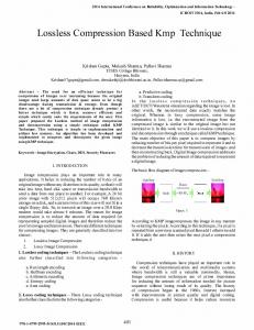
Fig. 1. The x-coordinates of this 75 million vertex Double Eagle tanker range from −4.095 to 190.974. The coordinates above 128 have the least precision with 23 mantissa bits covering a range of 128. There is sixteen times more precision between 8 and 16, where the same number of mantissa bits only have to cover a range of 8.

the various properties and how they attach to the mesh. For large and detailed models this representation results in files of substantial size, which makes their storage expensive and their transmission slow. The need for more compact mesh representations has motivated researchers to develop techniques for compression of connectivity [24,7,19,6,14,8,10], of geometry [23,24,6,9,10], and of properties [22,2,15,16]. The most popular compression scheme for triangulated surface meshes was proposed by Touma and Gotsman [24]. It was later generalized to both polygonal surface and hexahedral volume meshes [8–10]. It tends to give very competitive bit-rates and continues to be the accepted benchmark coder for mesh compression [11]. Furthermore, this coding scheme allows single-pass compression and decompression for out-of-core operation on gigantic meshes [12]. While connectivity is typically encoded in a lossless manner, geometry compression tends to be lossy. Current schemes quantize floating-point coordinates and other properties associated with the vertices onto a uniform integer grid prior to predictive compression. Usually one can choose a sufficiently fine grid to capture the entire precision that exists in the data. However, the original floating-point values will change slightly. Scientists and engineers typically dislike the idea of having their data modified by a process outside of their control and therefore often refrain from using mesh compression altogether. A more scientific reason for avoiding the initial quantization step is a nonuniform distribution of precision in the data. Standard 32-bit IEEE floatingpoint numbers have 23 bits of precision within the range of each exponent (see Figure 1) so that the least precise (i.e. the widest spaced) numbers are those with the highest exponent. If we can assume that all samples are equally accurate, then the entire uniform precision present in the floating-point samples can be represented with 25 bits once the bounding box (i.e. the highest exponent) is known. But if this assumption does not hold because, for example, the mesh was specifically aligned with the origin to provide higher precision in some areas, then uniform quantization is not an option. Finally, if neither the precision nor bounding box of the floating-point samples is known in advance it may be impractical to quantize the data prior to 2

compression. Such a situation may arise in streaming compression, as it was envisioned by Isenburg and Gumhold [12]. In order to compress the output of a mesh-generating application on-the-fly, one may have to operate without a-priori knowledge about the precision or the bounding box of the mesh. In this paper we investigate how to compress 32-bit IEEE floating-point coordinates with predictive coding in a completely lossless manner. The initial quantization step is omitted and predictions are calculated in floating-point arithmetic. The predicted and the actual floating-point values are broken up into sign, exponent, and mantissa and their corrections are compressed separately with context-based arithmetic coding [25]. As the quality of predictions varies with the exponent, we use the exponent to switch between different arithmetic contexts. We report compression results for single-precision floating-point coordinates predicted with linear predictions. However, our coding technique can also be used for other types of floating-point data or in combination with other prediction schemes. The achieved bit-rates for lossless floating-point compression nicely complement those resulting from uniformly quantizing with different precisions. Hence, our approach is a completing rather than a competing technology that can be used whenever uniform quantization of the floatingpoint values is—for whatever reason—not an option. Compared to the preliminary results of this work that were reported in [13] we achieve improved bit-rates, faster compression and decompression, and lower memory requirements. Furthermore we include a detailed comparison between the proposed compression scheme, simpler predictive approaches, and nonpredictive gzip compression. This comparison shows that current predictive techniques are not always the best choice. They are outperformed by gzip on data sets that contain frequently reoccuring floating-point numbers. The remainder of this paper is organized as follows: In the next section we give a brief overview of mesh compression. In the Section 3 we describe how current predictive geometry coding schemes operate. In Section 4 we show how these schemes can be adapted to work directly on floating-point numbers. In Section 5 we report compression results and timings. The last section summarizes our contributions and discusses current and future work. 2

Mesh Compression

The three-dimensional surfaces and volumes that are used in scientific simulations or engineering computations are often represented as irregular meshes. Limited transmission bandwidth and storage capacity have motivated researchers to find compact representations for such meshes and a number of compression schemes have been developed. Compression of connectivity and geometry are usually done by clearly separated, but often interwoven techniques. The connectivity coder [24,7,19,6,14,8,10] is usually the core component of a compression engine and drives the compression of geometry [23,24,6,9,10] and properties [22,15,16]. Connectivity compression is lossless due to the combinatorial nature of the data. Compression of geometry and properties, how3

ever, is lossy due to the initial quantization of the floating-point values. All state-of-the-art connectivity compression schemes grow a region by encoding adjacent mesh elements one after the other until the entire mesh has been conquered. Most compression engines use the traversal order this induces on the vertices to compress their (pre-quantized) positions with a predictive coding scheme. Instead of specifying positions individually, previously decoded positions are used to predict the next position and only a corrective vector is stored. Virtually all predictive coding schemes used in industry-strength compression engines employ simple linear predictors [3,23,24]. Recently we have seen a number of innovative, yet much more involved approaches to geometry compression. There are spectral methods [17] that perform a global frequency decomposition based on the connectivity, there are space-dividing methods [4] that compress connectivity-less positions using a k-d tree, there are remeshing methods [18,5] that compress a regularly parameterized version instead of the original mesh, and there are high-pass methods [21] that quantize coordinates after a basis transformation with the Laplacian matrix. We do not attempt to improve on these “lossy” schemes. Instead we show how predictive geometry compression schemes [23,24,6,9,10] can be adapted to compress floating-point coordinates in a lossless manner. 3

Predictive Geometry Coding

The reasons for the popularity of linear prediction schemes are that they are easy to implement robustly, that compression and decompression are fast, and that they deliver good compression rates. For several years already, the simple parallelogram predictor [24,9] (see Fig. 2) has been the accepted benchmark that many recent approaches are compared against. Although better compression rates have been reported, in practice it is often questionable whether these gains are justified given the sometimes immense increase in algorithmic and asymptotic complexity of the coding scheme. Furthermore these improvements are often specific to a certain type of mesh. Some methods achieve significant gains only on models with sharp features, while others are only applicable to smooth and sufficiently densly sampled meshes. Predictive geometry compression schemes work as follows: First all floatingpoint positions are converted to integers by uniform quantization with a userdefined precision of for example 12, 16, or 20 bits per coordinate. This introduces a quantization error as some of the floating-point precision is lost. Then a prediction rule is applied that uses previously decoded integer positions to predict the next position. Finally, an offset vector is stored that corrects the difference between predicted and actual integer position. The values of these corrective vectors tend to cluster around zero. This reduces the variation and thereby the entropy of the sequence of numbers, which means they can be efficiently compressed with, for example, an arithmetic coder [25]. The simplest prediction method predicts the next position as the last position, and was suggested by Deering [3]. While this technique, also known as 4

-1.01 N = 278.06 0.03

N new position

P = A–B +C predicted position

-1.01 1 7f 0147ae

-0.89 1 7e 63d70a

-0.89 P = A – B + C = 278.07 -0.01

sign

-1.32 A = 277.24 0.01

-0.33 C = 277.02 0.03

mantissa

exponent

278.06 0 87 0b07ae

278.07 0 87 0b08f6

the value of each component is reported in hexadecimal -0.76 B= 276.19 0.05

0.02 0 79 75c28f

-0.01 1 78 23d70a

function calls when compressing with encode( N , P ) comp_signexpo( true, 7f, 7e ) compress( signexpo[ 7e ], 5 ) comp_mantissa( 7f, 0147ae, 0 ) compress( mantissa_k[ 7f ], 11 ) compress( mantissa_bits[ b ], d1d ) compress( mantissa_bits[ 11 ], 2e )

comp_signexpo( true, 87, 87 ) compress( signexpo[ 87 ], 4 ) comp_mantissa( 87, 0b07ae, 0b08f6 ) compress( mantissa_k[ 87 ], 9 ) compress( mantissa_bits[ 9 ], b7 )

comp_signexpo( false, 79, 78 ) compress( signexpo[ 78 ], 0 ) compress( exponent, 79 ) comp_mantissa( 79, 75c28f, 0 ) compress( mantissa_k[ 79 ], 14 ) compress( mantissa_bits[ b ], 2e1 ) compress( mantissa_bits[ 14 ], 171 )

Fig. 2. The parallelogram predictor uses the vertices of a neighboring triangle to predict the next vertex. Only a small correction (here: the red arrow) needs to be encoded. The coordinates are broken up into sign, exponent, and mantissa components and differences between actual and predicted value are compressed separately using context-based arithmetic coding. The three components for actual and predicted x, y, and z coordinates are reported in hexadecimal. The function calls refer to the pseudo code from Figure 4. Compressing the difference between a vertex coordinate and its prediction requires between three and five calls to the arithmetic coder.

delta-coding, makes as a systematic prediction error, it can easily be implemented in hardware. A more sophisticated scheme is the spanning tree predictor by Taubin and Rossignac [23]. A weighted linear combination of two, three, or more parents in a vertex spanning tree is used for prediction. By far the most popular scheme is the parallelogram rule introduced by Touma and Gotsman [24]. A position is predicted to complete the parallelogram that is spanned by the three previously processed vertices of a neighboring triangle. The first vertex of a mesh component has no obvious predictor. We predict its position using the position that was processed last or – if this is the first vertex of the entire mesh – as zero. There will be only one such null prediction per mesh component. Also the second and the third vertex of a mesh component cannot be predicted with the parallelogram rule. We predict their position as that of a previously processed vertex to which they connect by an edge. There will be only two such delta predictions per mesh component. For all following vertices of a mesh component we use the parallelogram predictor. To maximize compression it is beneficial to compress correctors of the less promising null and delta predictions with different arithmetic contexts [9]. For meshes with few components this hardly makes a difference, but the Power Plant and the Double Eagle tanker each consist of millions of components. Predictive compression does not scale linearly with increased precision. Such techniques mainly “predict away” the higher-order bits. If more precision (i.e. low bits) is added the compression ratio (i.e. the compressed size in proportion to the uncompressed size) increases. This is demonstrated in Table 3, which reports bit-rates for parallelogram predicted geometry at different quantization 5

-0 .5 1 7E 000000

0 -½ ½ -1 1

- 4 .0 1 81 000000

-1 6 .0 1 83 000000 - 8.0

-16.0

- 8 .1 1 82 01999a

- 7 .9 1 81 79999a

- 4.0

2 .0 0 80 000000 2.0

- 2.0

- 0 .0 5 1 7a 4ccccd

4.0

0 .1 5 0 7c 19999a

8 .0 0 82 000000 8.0

16.0

1 2 .6 0 82 49999a

1 2 .8 0 82 4b3333

Fig. 3. The non-uniform distribution of floating-point numbers implies that the same absolute prediction error of, for example, 0.2 results in differences that vary drastically with the magnitude (i.e. the exponent) of the predicted numbers.

levels: the achieved compression ratios increase with increasing precision. The initial quantization step that maps each floating-point number to an integer makes predictive coding simple. The differences between predicted and actual numbers are also integers and the same absolute prediction error always result in the same difference. When operating directly in floating-point, predictive coding is less straight-forward. The non-uniform distribution of floatingpoint numbers makes compression of the corrective terms more difficult in two ways: First, the difference between two 32-bit floating-point numbers can in general not be represented by a 32-bit floating-point number computed using floating-point arithmetic without loss in precision. Second, the same absolute prediction error results in differences that vary drastically with the magnitude of the predicted number, as illustrated in Figure 3. For the largest numbers there will only be a difference of a few bits in the mantissa, but for smaller numbers this difference will increase. Especially when the sign or the exponent were miss-predicted we can not expect any correlation between the mantissas. Miss-predictions of the exponent become more likely for numbers close to zero. Here also the sign may often be predicted incorrectly. 4

Predictive Floating-Point Compression

In order to compress a floating-point coordinate using a floating-point prediction without loss we split both numbers into sign, exponent, and mantissa and then treat these components separately. For a single-precision 32-bit IEEE floating-point number [1], the sign s is a single bit that specifies whether the number is positive (s = 0) or negative (s = 1), the exponent e is an eight bit number with an added bias of 127 where 0 and 255 are reserved for unnormalized near-zero and infinite values, and the mantissa m is a twenty-three bit number that is used to represent 223 uniformly-spaced numbers within the range associated with a particular exponent. We compress the differences in sign, exponent, and mantissa between a floatingpoint number and its prediction component by component with a contextbased arithmetic coder. Especially for the mantissa, the success of the prediction is tied to the magnitude (i.e. the exponent) of the number (see Figure 3). The same absolute prediction error results in a smaller difference in mantissa for numbers with larger exponents. In particular, this difference doubles/halves when the exponent is decreased/increased by one. This is because the spac6

ing between consecutive floating-numbers changes with the exponent, so that more/less of these spacings are required to express that difference. We account for this by switching arithmetic contexts based on the exponent. This prevents the high-entropy correctors from predictions for numbers with small exponents from spoiling the potentially lower entropy of correctors from predictions for numbers with higher exponents. void comp mantissa(int expo, int a, int p) { // c will be within [1-223 ... 223 -1] int c = a - p; // wrap c into [1-222 ... 222 ] if (c