LOW COMPLEXITY VIDEO CODEC FOR MOBILE VIDEO CONFERENCING .... of two input complex signals, let's call them respectively. A = Ar + jAi , and B = Br ...
LOW COMPLEXITY VIDEO CODEC FOR MOBILE VIDEO CONFERENCING Andrea Molino+, Fabrizio Vacca+ , Mainak Biswas∗ and Truong Q. Nguyen∗ + CERCOM
– Dipartimento di Elettronica Politecnico di Torino – Italy http://www.vlsilab.polito.it
ABSTRACT Current video coding techniques provide very good performance both in terms of compression ratio as well as image quality. In practice, the required computational complexity tends to be significant. Environments that have significant power or computational performance restrictions would benefit from improved coding and decoding, especially if complexity is kept manageably low. In this paper the design of a symmetric codec with significantly low complexity is shown, particularly suited and optimized for mobile environments. Low–complexity algorithms and approaches are employed, and results obtained with a software model are provided both in terms of complexity as far as visual quality.
∗ Electrical
and Computer Engineering Dept. University of California – San Diego (US) http://videoprocessing.ucsd.edu
footprints of the encoder can be controlled to match the resource availability of current wireless terminals. As far as the complexity is concerned, being able to control the rate without the need for any re–coding step decreases the computational requirements on the encoder side; on the other hand, this also leads to a reduction of rate allocator output buffer size. The paper is organized in the following sections. The encoding of the video signals is described in section 2 that includes the motion estimation, rate allocation and error encoding. Section 3 describes the decoder and the frame rate up conversion and images scaling done on the decoded video. Finally, in section 4 the experimental results and some conclusions are drawn.
1. INTRODUCTION Digital communication and storage of image data is a difficult task due to the sheer volume of digital data required to accurately describe a single frame of an image. In video, the amount of data is exorbitant. Image coding seeks to make the communication and/or storage image data manageable. Communication resources, for example, have limited bandwidth. This is especially true in wireless communication media. There are tradeoffs in image data coding. Reducing the size of the data should not, for example, degrade the image quality beyond an acceptable metric. Also, the computational cost and speed must be managed, especially in devices where computational resources and power resources are to be conserved. Wireless handsets present an example of a difficult environment for implementation of video data communications. Modern examples of video encoding approaches include MPEG–4 [1] and H.264 [2]. In particular the latter has been specifically designed for video transmission over packet networks. However, these video standards are designed and optimized for broadcasting scenarios (server and client transmission). Both MPEG–4 and H.264 have been designed as highly asymmetric codecs, where the encoder complexity is much higher than that of the decoder. Such design enables fairly simple decoder implementations, suitable for the integration on mobile applications. However in a two–way real time communication application (as in videoconferencing), both the encoder and the decoder need to be integrated on the same platform. The optimization of an H.264 video codec is a challenging problem [4]. For example an assembly– optimized version of the reference H.264 on an Intel Pentium 4 (running at more than 2 GHz) achieves:0.85 frames per second encoding a (352x240) CIF sequence, but 30 frames per second decoding the same sequence. This paper details the design of a symmetric codec with significantly low complexity. This video codec is particularly suited and optimized for mobile environments. Memory
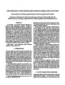
2. ENCODER OPERATION In order to better understand the encoder structure Fig 1, three different functional parts can be identified, namely the input processing, the frame coding and the motion estimation and compensation. The first is devoted to perform preliminary processing to the input frames, such as de–noising, down–sampling etc. The second part deals with the coding of an image frame using techniques similar to still image coding. Besides, this part is also responsible for the efficient coding of the prediction error, when the motion estimation process is employed. The last functional part estimates the motion in the input sequence. In particular the motion estimation block is able to determine the motion between a reference frame and the current one: this motion information will be passed to the motion compensation engine as a motion vector field. The motion compensation by itself will apply this motion vector field to the reference frame obtaining a predicted version of the current frame. Finally, the frame coding block will be used to encode the difference between the current frame and the motion–compensated version. 2.1 Input Pre–processing The preprocessing block is the first stage in the encoder chain: the main goal of this block is provide the encoder engine a frame that can be either the original frame or a spatial down–sampled version of the original. When working at very low bit rates, the spatial down–sampling allows the following encoder blocks to work with smaller images, achieving better results in the overall visual quality. Otherwise, when a small amount of bits are allocated to the error frame, the compensated image can exhibit strong blocking artifact. Working under the same constraint with a down–sampled image, the resulting decoded (eventually up–sampled) image exhibit only blurrier shapes, which is less annoying than the presence of high–frequency artifacts. A down–sampling fil-
665
Intra / Inter
Input Frame
Rate allocator
Preprocessing WDR (or any other wavelet based entropy encoder)
Forward Wavelet Transform
-
1010… Output Buffer
Inverse Wavelet Transform Input processing Motion Compensation
Frame coding
Motion Vectors
Motion Estimation
Motion estimation and compensation
Reference Image
Figure 1: Block diagram of the video encoder ter must be inserted in this block to avoid aliasing. The option to select either a decimation filter or to use the Wavelet Transform Engine is provided in the described scheme. In the latter case the LL sub–band of the transformed image is taken as down–sampled frame. 2.2 Motion Estimation This block (figure 2) is devoted to find the motion vectors that represent the motion between two consecutive frames. In the described coder a low complexity motion estimation algorithm based on a FFT transform is used [6]. According to this algorithm, the FFT of the corresponding window in the two frames is calculated, and then the difference of the two relative phase planes is taken. This value is normalized and inverse transformed, obtaining a surface where the position of the maximum indicates the value of the estimated motion vector. Here it is interesting to note how, according to the aforementioned algorithm, it is necessary to compute a large number of phase difference among the transformed values. Video In
F (x,y) 1
Pre-process
FFT
F 2(x,y)
Delay
DOT Product
Normalize
IFFT
(PQ). This algorithm allows to avoid the computation of the two blocks dot product and normalization. Depending on the implementation platform, the PQ strategy can be activated or not, since it can produce advantages in an hardware or DSP implementation, while it is not convenient implementing the motion estimation block on a general purpose processor. The detailed description of the PQ method is described in the following subsection. It should be observed, however, as some changes and improvements over the original algorithms have been necessary in order to improve the accuracy of the method. However, any other phase estimation / evaluation method will work as well. To avoid situations where, due to highly noisy images or too big motion, the obtained MV are not corresponding to the true motion, we insert in the coder the possibility of verifying the correctness of these vectors. With this option activated, the coder performs a test with the calculation of two SAD and evaluates if the moved block exhibit or not more correlation in the current frame respect to the original (not moved) position. 2.2.2 Phase Quantization This operation leads in approximating the phase difference of two input complex signals, let’s call them respectively A = Ar + jAi , and B = Br + jBi. The first step of the algorithm is to divide the complex plane in eight slices of π /4 of amplitude, and assigning each input sample to one of these slices. This operation is effortless, since it can be done computing only three comparisons each input coefficient (for example, for the A input it is necessary to evaluate the expressions: Ar > 0, Ai > 0, Ar > Ai). In this way we can evaluate the phase difference only looking at the relative position of the input samples, but the obtained precision is coarse ±4π . The second step leads in rotating clockwise A and B by an angle multiple of π4 , and translating them in the first slice (0- π4 ). In this way we loose the information relative to the first approximation. The next step is to compute Am and Bm . In this way the incertitude interval is expanded by a factor m since the obtained results have phase which is m times the original one. Now the slice–lookup operation can be repeated and a better approximation of the phase difference can be achieved. The last two steps (m–power and lookup operation) can be reiterated as many times as is needed to reach the sought precision.
Motion Estimator Obtain Candidate Vectors
Motion Vectors
Figure 2: Phase correlation based motion estimator 2.2.1 Phase extraction Use of actual phase difference presents at least two major disadvantages. Firstly, for each difference both a division and an arctangent are needed; besides, in order to avoid numerical misrepresentation, the employment of a floating–point arithmetic is highly advisable. However these requirements are anti–thesis to the requirement of the low complexity. For the aforementioned reason an effective approximation for the phase difference step is employed, called phase quantization
2.3 Rate Allocator This block is devoted to distribute the overall bit budget among the different frames. Different frames need different amount of bit to be encoded since an equal distribution can penalize the frames with high motion inside (error frames with high entropy). The rate controller is mainly composed of an output buffer and a control unit. The control unit (CU) must avoid situations where the buffer is full or empty, given that the encoded stream is sent at a fixed bit rate, and the Encoding Engine is a variable bit rate source. In our coder we extract from the encoding engine block a metric giving us information about how well the current frame has been predicted, and then we assign to this frame (and then to the relative error frame) a quantity of bit proportional to the inverse of this metric. In this way imperfectly predicted frames (with an expected significant energy in the error frame) is given more budget, and vice versa for the well predicted ones. The
666
metric that is used to evaluate the correctness of the prediction is the average of the peaks found during the FFT–based motion estimation step, in the phase plane domain. The rate allocator state–machine then operates as follow: At the beginning of the transmission, the quantity prec bit budg is calculated: this is the amount of bit to give each frame on the hypothesis of equal distribution. Then, for each frame n in the sequence. The motion estimation function returns the values of the peaks (magnitude) found in the entire frame, then the average of these values is calculated Peak(n). In a variable inside the rate allocator the ”history” Hist(n) of this value is stored, as an average among the N past frames Hist(n) = N1 ∑Ni=1 Peak(n − i). A factor, called
Intra / Inter
Intra frame / error frame
The value of Hist(n) is upgraded with the current value of Peak(n). The values of N and k can be changed, making the rate allocator more or less reactive to the changes in the sequence. This metric, according to the simulations, is a good indicator of the visual quality of a predicted frame Fig. 3). The second reason to use this metric is that there is almost no need for additional computation, since the calculation of the phase peak has to be done anyway in the motion estimation block. In addition to this strategy, the rate allocator can skip a given frame in cases when the buffer level is more than a programmable threshold, or the expected error energy is more than another programmable threshold. In these cases the decoder duplicates the previous frame, avoiding situations where the visual quality can be degraded.
Inverse Wavelet Transform
Postprocessing
Rec. video
Reference Image Frame decoding Motion Vectors
Motion compensation and FRUC
Motion Compensation Motion Vectors Processing
Hist(n) γ (n), is calculated as γ (n) = Peak(n) . A bit budget proportional to this factor is given to the current frame :
bit budg(n) = γ k (n) ∗ prev bit budg(n)
Inverse W DR
Original / FRUC
Interpolated Frame (FRUC)
Output processing
Figure 4: Block diagram of the video encoder Another interesting feature of the WDR is the possibility to create embedded bit–stream. This could enable the creation of multiple descriptors for each frame, providing a bandwidth scalable video source. Lastly, if the memory requirement is the main concern, the transformed image can be divided in to smaller blocks and the WDR algorithm can be independently applied to each of them. In order to improve the effectiveness of the WDR algorithm in the inventive scheme, some enhancements have been applied. • A different scanning order has been employed in order to take into account the sequence’s structure. • A particular symbol encoding has been invented for the significance pass in order to reduce the number of bits needed when a zero distance has to be emitted. • A different coding has been employed for the End–Of– Significance symbol to reduce the number of bits emitted. In the WDR encoder we keep an additional buffer to store the reconstructed version for the current block. In this way it is possible to avoid the presence of a separate decoder block on the feedback loop. 3. DECODER At the other end of the transmission chain, a decoder block is required in order to reconstruct the video sequence. Similarly to the encoder block, it is possible to identify three distinct functional parts (see figure 4): Frame decoding, Motion compensation / Frame Rate Up–Conversion (FRUC) and Output post–processing. 3.1 Frame Rate Up–conversion
Figure 3: Confidence test for the rate controller strategy Peak(n) vs PSNR(n) for first 50 frames in Foreman sequence (very–low bitrate case). 2.4 Entropy Encoder In order to reduce the amount of information to be transmitted, a suitable entropy coding block is needed after the transform stage. Wavelet Difference Reduction (WDR) [3] method has proven to be particularly effective on natural images. Additionally, it can act as a rate–controlled, multiplier– less quantization stage. These characteristics will make the WDR the natural solution to be employed in the video codec.
The idea behind the FRUC is to obtain a higher frame rate starting from a lower one. This feature could be beneficial especially in a low bit–rate scenario (as the wireless one): as an example, the encoder can send a 5 frame per second (fps) sequence and, by the means of this technique, the decoder can produce the 10 fps version, leading to an improvement of the visual quality. Since our primary goal in the inventive scheme is to minimize the computational complexity, we develop a custom solution, starting from the work presented in [5]. The invented FRUC technique works only on the motion vector field, producing an interpolated version of it. The obtained motion vectors for the reconstructed frame are simply the average of the past and the current value of the motion vectors in the corresponding block.
667
Codec H.263 H.264 MJPEG Proposed
Avg. quality (dB)
Frame rate (frame/s)
Energy/frame (J/frame)
35.4 36.8 N/A 34.3
11.12 0.26 28.17 46.15
125 3.19 1.20 0.67
Table 1: Encoder profile results for the first case (QCIF video, 12 fps, 16 kbps). Please note how no average quality is specified for the MJPEG case since the visual quality was completely unacceptable under the test conditions. 3.2 Output Post–Processing This option allows the decoder to spatial up–sample the reconstructed image. If this option is activated together with the Input Frame down–sampling, the decoder can produce a reconstructed sequence with the same size of the original one. As in the down–sampling block, it is possible to employ either an up–sampling FIR filter or the IWT engine, using the decoded image as LL wavelet subband. 4. SIMULATION RESULTS AND CONCLUSIONS The proposed video coder has been implemented resorting to the ANSI C programming language. As far as the development complexity is concerned, this phase lasted for 3 months, leading to around 9k code lines, both for the encoder and the decoder parts. Through the availability of this running model, several experiments were possible to compare our solution with other well–known international standards. As explained in the previous sections, the first goal of this coder was to achieve good visual quality expecially in very– low–bitrate scenarios. Besides the video quality, the coder’s simplicity and the efficiency were considered primary objectives as well. Additionally, the coder should perform particularly well in a walkie–talkie–like applicative context (bidirectional, real–time video transmission), expecially with “head– and–shoulders” video sequences. Given these premises, two different test situations have been identified: • Transmission of a QCIF video (176 × 144), 10 to 12 fps using 16 kbit/s data rate (luma component only). The data bandwidth can be increased up to 24 kbit/s if also the chrominance components are present. • Transmission of an SQCIF video (128 × 96), 10 to 12 fps with just 9.6 kbit/s bandwidth (luma components only). Also in this case we will extend the data rate up to 16 kbit/s if the other two color components will be included. After this we have identified some proper test sequences, extracted from the “classical” ones. On this set of sequences we have carried out all the benchmarks and comparisons. The three possible competitors for the proposed algorithm were H.263, H.264/AVC and Motion JPEG (MJPEG). The choice of the first has been almost “natural” due to its widespread diffusion in bidirectional video communications. H.264 has been included as a significant example of state–of– art video codec, while Motion JPEG represents an example of ultra–low–complexity encoder. For all these three codecs we used an ANSI C implementation, without the use of any assembly–optimized library or function. An Intel P4 1.4 GHz with 1 GB SDRAM has been employed to carry out the profile measures. In table 1 the obtained results for the QCIF
case are shown. As far as the SQCIF results are concerned, they have been omitted to suits the space constraints. Observing the data in this table, some interesting figures can be emphasized. Firstly, even if MJPEG could seem attractive for its simplicity, it lacks the proper coding efficiency, leading to a very poor visual quality. On the other hand, both H.263 as well as the state of the art H.264 were able to reach an interesting quality even working at a such low bitrate. However, the computational complexity of the H.264 encoding process it’s quite impressive considering the fact that, even on a P4 processor, a frame rate of only 0.26 fps has been reached (QCIF case). H.263, on the other hand, represents a good compromise between coding efficiency and complexity: we have been almost able to achieve real–time video encoding rate using only the ANSI C version of the encoder (11.12 fps for 12 fps video). The proposed video coder exhibits an average quality loss of 1.1 dB with respect to H.263 under the same working conditions. The surprising fact is how it can be efficient if one considers that an encoding rate of almost 46 fps have been achieved. It is important to stress that neither this code has been optimized for the P4 processor: the coder has been completely written in portable ANSI C. Finally, another interesting, even if unusual, comparison can be made considering the amount of energy needed to encode a single frame. This estimation has been carried out referring to the Intel P4 data book (for the power consumption data) and using the profile results. The proposed coder performs quite well even under this standpoint, making its use particularly attractive in energy–constrained environments. REFERENCES [1] ISO/IEC 14496–2 ”Coding of audio–visual objects. Part 2: Visual”, ISO/IEC JTC1. MPEG–4 Visual version 1, April 1999; Amendment 1 (Version 2), February 2000. [2] Joint Video Team of ITU–T and ISO/IEC JTC 1, ”Draft ITU–T Recommendation and Final Draft International Standard of Joint Video Specification (ITU–T Rec. H.264 — ISO/IEC 14496–10 AVC)”, Joint Video Team (JVT) of ISO/IEC MPEG and ITU–T VCEG, JVT– G050, March 2003. [3] J. Tian and R. O. Wells, Jr. ”Embedded Image Coding Using Wavelet Difference Reduction”, Wavelet Image and Video Compression, P. Topiwala, Editor, 289–301, Kluwer Academic Publishers, 1998. [4] X. Zhou, E. Q. Li, and Y. Chen, ”Implementation of H.264 Decoder on General–Purpose Processors with Media Instructions”, to appear in the Proceedings of SPIE Conference on Image and Video Communications and Processing, vol. 5022, 2003 [5] G. Dane and T. Q. Nguyen, ”Motion Vector Refinement for Frame Rate Up Conversion”, University of California San Diego Jacobs School of Engineering Research Review, 2003 1989 [6] G. A. Thomas, ”Television motion measurement for DATV and other applications”, BBC RD 1987/11
668