Low-cost and open-source solutions for automated image orientation – a critical overview Fabio Remondino1, Silvio Del Pizzo2, Thomas Kersten3, Salvatore Troisi2 1
3D Optical Metrology (3DOM), Bruno Kessler Foundation (FBK), Trento, Italy
[email protected], http://3dom.fbk.eu 2
3
Parthenope University of Naples, Dept. of Applied Science, Naples, Italy @uniparthenope.it
Photogrammetry & Laser Scanning Lab, HafenCity University Hamburg, Germany
[email protected], http://www.hcu-hamburg.de/geomatik/kersten
Abstract. The recent developments in automated image processing for 3D reconstruction purposes have led to the diffusion of low-cost and open-source solutions which can be nowadays used by everyone to produce 3D models. The level of automation is so high that many solutions are black-boxes with poor repeatability and low reliability. The article presents an investigation of automated image orientation packages in order to clarify potentialities and performances when dealing with large and complex datasets. Keywords: photogrammetry, computer vision, orientation, low-cost, opensource
1 Introduction 3D model generation of artifacts, monuments or large environments is becoming a common practice for applications like documentation, digital restoration, visualization, inspection, planning, AR/VR, gaming, entertainment, etc. 3D modeling should be intended as the entire procedure which produces a three-dimensional product starting from surveyed data (reality-based approach) or other sources of information. Data can be recorded with digital cameras or active sensors leading to the well-known image-based [1] or range-based [2] approaches, respectively. The image-based approach is generally considered a low-cost method (in particular for terrestrial applications), flexible, portable and capable of reconstructing lost scenarios simply using archives images [3]. In the recent months different solutions have become available for the automated processing of images and the derivation of 3D information and models. The processing mainly includes image orientation and dense 3D reconstruction with an incredible level of automation. The article investigates the performances and reliability of some low-cost commercial and open-source packages able to automatically process large blocks of images and retrieve the unknown camera poses. Different datasets are used comparing the software outcomes in terms of visual and metric analyses.
1.1 Related works Multiple image orientation is the most important (fundamental) task in photogrammetry and computer vision. It often includes the simultaneous camera calibration procedure leading to the well-known self-calibration method. The accuracy and the reliability of image orientation and camera calibration significantly influence the quality of all subsequent processes such as 3D point determination and 3D modelling. Thus orientation and calibration of cameras [4] is a prerequisite for many applications. These processes are already fully automatic since the early 1990’s in close-range photogrammetry for laboratory and industrial applications using coded targets or markers [5]. However, in several other (outdoor) fields such as architecture, archaeology and Cultural Heritage, coded targets cannot be employed. In these cases, the tie point identification for the determination of the Exterior Orientation (EO) is more complex and need to be solved, preferably, using fully automatic image matching procedures. On the other hand, the precise measurements of control points for the scaling and geo-referencing of the image block (absolute orientation) is still a manual (interactive) task. We have to distinguish between image orientation and camera calibration procedures in photogrammetry and computer vision. The photogrammetry community put more emphasis on accuracy and reliability in image orientation and camera calibration procedures with less prominence on automation as the main applications lay in the fields of mapping, cartography, documentation and monitoring. On the other hand the computer vision community focuses more on the automation aspect of these processes often overlooking the geometric quality of the results as the main applications are in the fields of robotics and inspection where automated processing is a mandatory need. Photogrammetry uses a pinhole camera model generally with ten parameters for the Interior Orientation (IO): principal point (2 parameters), principal distance (1), radial lens distortion (2-3), tangential distortion (2), affinity (1) and shearing (1). Computer Vision uses projective geometry and the interiors are limited to the principal point (2), principal distance (1) and radial lens distortion (1-2) coefficients. One of the first introductions of the photogrammetric camera model was presented by Brown [6]. A remarkable paper covering the whole historical development of camera calibration techniques was given by Clarke & Fryer [7] including an exhaustive literature survey. An overview of current approaches adopted for camera calibration in close-range photogrammetry and computer vision discussing operational aspects for self-calibration is presented in Remondino & Fraser [8] while in [9] the state-of-the-art of automated camera calibration is given. Camera calibration must be computed with an ad-hoc image network as a typical set of images for 3D reconstruction purposes do not allow the correct determination of all the interior parameters. Nevertheless the computer vision community favorites the field selfcalibration approach leading to the so called Structure from Motion (SfM) method, which includes the simultaneous determination of (interior and exterior) camera parameters and 3D scene’s structure. Camera calibration is generally performed by means of coded targets or checker-boards, in order to achieve higher accuracy in the tie point identification and camera parameters estimation. A markerless camera calibration approach has been presented in [10].
On the other hand, automatic markerless orientation of terrestrial images has been available in the photogrammetric community in the recent years [11-15]. But the largest developments and innovations came from the Computer Vision community since the end of the 90’s, with the SfM approach [16-23]. The derived SfM 3D reconstructions are generally useful mainly for visualization, object-based navigation or other similar purposes and not for photogrammetric and mapping purposes. Nowadays, due to these advances as well as computer technology and performance improvements, huge numbers of images can be automatically oriented in an arbitrarily defined object coordinate system, using a variety of algorithms which are often available as open-source software (VisualSFM, Bundler, Apero, Insight3D, etc.) or as free web service (Microsoft Photosynth, Autodesk 123D Catch Beta, My3DScanner, Hypr3D, Arc3D, etc.). Different packages, after the determination of the camera parameters, provide also a 3D reconstruction method able to deliver dense point clouds or polygonal models as PMVS2 [24] and MicMac [25]. This level of automation in the 3D reconstruction pipeline from images has also led to collaborative mapping and modeling communities and projects like PhotoCity [26] or the Volunteered Geographic Information (VGI) [27]. On one hand automation and web-based processing helps to save human resources in data processing, but on the other hand there is no guarantee on aspects such as data privacy and 3D model quality. On the commercial side, packages like PhotoModeler Scanner and Agisoft PhotoScan have recently appeared on the market, providing automatic image orientation, camera calibration and 3D reconstruction of objects from image sequences. However, an evaluation of precision, reliability and repeatability of such automatic procedures is missing and it would be quite useful for non-experts facing the image-based 3D reconstruction approach.
2 Image triangulation In photogrammetry the term image triangulation generally means the procedure to orient a set of images in order to derive the exterior (and eventually interior) parameters. The procedure requires a reliable set of image correspondences (tie points), manually or automatically extracted, which are the main input for a successive non-linear least squares minimization named bundle adjustment. The main problems precluding the existence of reliable commercial approaches are the presence of convergent images, unpredictable baselines and scale variations, lighting changes, homogeneous textured areas, repetitive patterns, complex object configurations, etc. These effects give strong perspective deformations and make the automated tie point identification a challenging task. 2.1 Image correspondences identification The identification of the image correspondences (Fig. 1) starts with the extraction of points or regions of interest using dedicated area-based or feature-based algorithms. Nowadays SIFT [28] and SURF [29] algorithms provide highly distinctive features invariant to image scaling and rotations with an associate descriptor (64- or 128-dimensional vector) to each extracted image feature. Corresponding points are then found by comparing the descriptors with an exhaustive
analysis of all possible image combinations. Rigorous but slow procedures (e.g. quadratic matching) or fast but approximate methods (e.g. kd-tree search) can be used. In order to remove possible outliers, robust estimators (RANSAC, MAPSAC, LMedS, etc.) are employed to validate the epipolar constraint encapsulated into the fundamental matrix F or the essential matrix E (if interior orientation parameters are known) or the trifocal tensor T (in case of image triplets). Once corresponding points for each image pair (or triplet) are available, they are organized into tracks and the comparison of the numerical values (pixel) of all image points gives the set of image correspondences for the entire block or sequence. feature extraction: SIFT-like, SURF, etc. quadratic matching or kd-tree descriptor comparison and pairwise correspondences extraction
robust outlier rejection: E/F matrix or T tensor with RANSAC, son MAPSAC or LMedS method concatenation of all image combinations and extraction of image correspondences for the entire image block
bundle adjustment Fig. 1. Typical workflow for the automated extraction of image correspondences.
2.2 Bundle adjustment Once the image correspondences are extracted, their 3D (object) coordinates are computed by means of a bundle adjustment method. The bundle adjustment method was conceived in the photogrammetric community in the 50’s [30] and become the standard solution for 3D reconstruction problems in the 80’s. During recent years it has increasingly been used also in the computer vision community [31-33]. A bundle adjustment is an optimization problem on the sought 3D structure and camera parameters (positions, orientations and eventually the internals) in order to estimate a 3D reconstruction which is optimal under certain assumptions: if the error in the image measurements is zero-mean Gaussian, then the bundle adjustment is the maximum likelihood estimator. The optimal estimation is found by minimizing a cost function which quantifies the model fitting error and simultaneously estimate the extracted 2D features in 3D and the camera parameters. Generally a bundle adjustment is formulated as a non-linear least squares problem with the cost function being quadratic in the feature reprojection error (i.e. the sum of the squared differences between the measured and back-projected image points). The numerical solution to the problem of function minimization is generally sough with methods like Levenberg-Marquardt, Gauss-Newton or Gauss-Markov.
In the bundle adjustment a reference coordinate system must be defined leading to the datum (or gauge) definition problem. The datum definition problem is also called Zero-Order-Design problem [34]. A datum must be defined imposing some constraints that establish the origin, orientation and scale of the reference coordinate system. So the datum is generally given by fixing the seven parameters of a spatial similarity transformation. The datum is generally achieved with inner, minimal or over-constraints solutions: - inner constraints: the solution (also called free-network adjustment) is always chosen where the trace of the covariance matrix of the estimated parameters is a minimum. The geometric interpretation of the minimum trace is that there should not be any translation, rotation or scaling changes from the given approximate values of the unknown parameters, thus requiring very good initial values for the non-linear least squares problem. One of the advantages of a free-network adjustment is the fact that it can better identify the existence of certain un-modeled systematic error in the system, as the solution is not influenced by external factors. The free-network adjustment does not ensure the derivation of correct metric results so requiring a aposteriori scaling or similarity transformation. - minimal constraints: the constraints are said to be minimal if they do not introduce external information into the estimated parameters of the bundle adjustment. This is the typical datum definition with three Ground Control Points (GCPs) providing at least seven information, e.g. two points with X, Y, Z coordinates and one point with only the Z coordinate. - over constraints: if more than the seven necessary information is introduced in the adjustment, the sum of the squared residuals is invariably larger and there might be distortions into the estimated parameters (3D structure and camera parameters). So there are basically two main approaches to proceed when solving a bundle adjustment: 1. import at least three spatially well-distributed GCPs, treating them as weighted observations inside the least squares minimization. This approach is the most rigorous as (i) it minimizes the possible image block deformations and possible systematic errors, (ii) it avoids instability of the bundle solution (convergence to a wrong solution) and (iii) it helps in the determination of the correct 3D shape of the surveyed scene assuming no errors in the GCPs. 2. use a free-network approach and apply only at the end a similarity transformation in order to bring the image network results into a desired coordinate system. This approach is not rigorous: the solution is sought minimizing the trace of the covariance matrix, introducing the necessary datum with some initial approximations. As no external constraint is introduced, if the bundle solution cannot determine the right 3D shape of the surveyed scene, the successive similarity transformation would not improve the result, leading thus to some block deformations. The two approaches, in theory, are not equivalent and they can lead to totally different results. Indeed in the first approach, the quality of the bundle is only influenced by the redundant control information and additional check points can be used to derive some statistics of the adjustment. On the other hand, the second approach has no external shape constraint in the adjustment thus the solution is only based on (i) the integrity and quality of the multi-ray relative orientation and (ii)
initial approximations of the unknown parameters. Therefore the fundamental requirement is to have a good image network in order to achieve correct results in terms of computed camera parameters and scene’s 3D shape otherwise the aposteriori similarity transformation cannot compensate for any geometrical shape deformation.
3 Datasets and employed packages The used image sequences (Table 1 and Fig. 2) feature some real scenarios typical of surveying campaigns as well as two lab-sequences for quality and accuracy analyses. Different image resolution and digital cameras are employed with ground truth data represented by calibrated bars, Ground Control Points (GCPs), calibrated interior parameters and known shapes. Repetitive pattern (“Cerere”) and texturless scenes (“Railway”) are also present. Dataset name
# img
resolution (pixel)
focal (mm)
image type
dim. L x WxH (m)
CUBE
24
6048x4032
50
terr.
0.1 x 0.1 x 0.1
SPHERE
67
3008x2000
35
terr.
0.2
LIGHTHOUSE
119
3008x2000, 4256x2832
18, 85
terr.+ UAV
14x14x40
GCPs
CERERE
212
6048x4032
35, 50
terr.
15 x 30 x 10
-
RAILWAY
147
4256x2832, 4288x2848
20, 28
terr.
15x15x10
GCPs
NAVONA
92
4000x3000
6
terr.
50 x 250 x 15
calib. camera
ground truth calib. bar, calib. camera, known shapes calib. bar, known shapes
Table 1. Main characteristics of the employed datasets for the evaluation of the automated image orientation packages.
The automated image orientation packages used for the reported investigation are: - Agisoft Photoscan: developed by Agisoft LLC, it is a low-cost commercial software which allows to orient and match large dataset of images. Due to commercial reasons, few information about the used algorithms is available. - Apero: developed by the Matis laboratory of the French I.G.N (Institut Géographique National), it is an open-source software that joins a computer vision approach to provide an initial solution and a rigorous photogrammetric approach to achieve an optimum solutions with a classical Gauss-Newton bundle adjustment [14]. This software uses a modified SIFT++ feature extractor [35] and allows to choose between several camera model (Brown’s, fisheye, etc.). Apero is generally coupled with MicMac, an open-source dense image matching package [25]. - Bundler: developed by the University of Washington & Microsoft, it was created with the aim of reconstructing 3D scene using a huge number of images downloaded
from Internet with unknown internal parameters [36]. The software uses a typical SfM approach, with RANSAC to estimate the F matrix from the extracted SIFT features and reject possible outlier for every couple of images. Afterwards a custom minimization of the reprojection error is performed in order to solve a non-linear least squares problem and estimate nine camera parameters (three translations, three rotation, the focal length and two radial distortion parameters) for each image. - Photosynth: released by Microsoft Live Labs, it is a web-service optimized version of Bundler. It works like a black-box, simply uploading the images through an Internet website. -VisualSfM: developed by the University of Washington & Google Inc., it is a GUI application of a SfM software optimized to work with multicore architectures and on the GPU. The author uses their own feature extractor called SiftGPU [37] and the Multicore Bundle Adjustment [38] which combines the classical LevenbergMarquardt algorithm with the Preconditioned Conjugate Gradients algorithm [23]. The adjustment solves a non-linear least square problem to estimate eight camera parameters (three translations, three rotations, the focal length and one radial distortion parameter) for each image.
CUBE
CERERE
SPHERE
RAILWAY Fig. 2. An image for each of the employed datasets.
LIGHTHOUSE
NAVONA
4 Results, comparisons and analyses 4.1 Visual analysis of the orientation results A quick but often acceptable analysis of the adjustment results is a visual inspection of the retrieve camera poses and 3D object coordinates. For the “Cerere” and “Navona” sequences (Fig. 3 and 4), the visual analysis of the adjustment’s output reveals some problems for the SfM tools in case of long and complex sequences. The failure and divergence of the bundle adjustment can be due to different reasons like (i) estimation of a set of interior parameters for each image, (ii) sequential bundle
estimation and not global adjustment, (iii) wrong initialization, (iv) uncontrolled error propagation, etc. NAVONA AGISOFT: Oriented images: 92/92 # 3D tie points: 193451
PHOTOSYNTH: Oriented images: 92/92 # 3D tie points: 71068
BUNDLER: Oriented images: 92/92 # 3D tie points: 73020 APERO: Oriented images: 92/92 # 3D tie points: 334908 VISUALSFM: Oriented images: 56/92 # 3D tie points: 21334 Fig. 3. Visual analysis of the achieved orientation results for the Navona sequence (92 images, 12 Mpx, 6 mm nominal focal length): the correct closure of the image block vs the divergence and failure of the bundle solution.
4.2 Comparison of the calibrated interior orientation parameters The “Cube” and “Navona” datasets feature calibrated interior orientation parameters, derived with an ad-hoc image network and a photogrammetric bundle adjustment. The calibrated values have been compared with those derived with the different packages under evaluation in order to see their performances and reliability in self-calibration mode. Fig 5 shows the comparison results, for both sequences, showing the behavior of the focal length and the K1 value of the radial distortion. SfM tools compute a different set of interior parameters for each image, leading to very strange oscillation in the parameter’s value. This is quite unusual in photogrammetry where in case of a unique camera employed for the surveying, a unique set of interior parameters should be recovered by the bundle. This instability is more peculiar in particular for the “Cube” sequence which features an image network suitable for self-calibration (Fig.5, top). Moreover, the fact that a set of interior is determined for each image might lead to wrong undistorted images.
AGISOFT
CERERE
# 3D tie points: 926126
Oriented images: 212/212
# 3D tie points: 400528
Oriented images: 212/212
# 3D tie points: 1170618
Oriented images: 212/212
# 3D tie points: 6711547
Oriented images: 199/212
# 3D tie points: 194902
VISUALSFM
APERO
BUNDLER
PHOTOSYNTH
Oriented images: 212/212
Fig. 4. Visual analysis of the achieved orientation results for the Cerere sequence (212 images, 24 Mpx, 35 mm and 50 mm nominal focal length): correct joining of the internal and external networks vs divergence and failure of the bundle solution.
CUBE
NAVONA
Fig. 5. Comparison between the calibrated interior parameters and those derived with the field self-calibration. IO instability is clearly visible for SfM tools.
calib. bar (mm) RMSE (px) XYZ (mm)
Reference 0.325 0.021
Agisoft 0.301 2.212 0.143
CUBE Photosynth -0.547 7.149 0.611
Bundler 0.220 3.961 0.365
Apero -0.379 3.440 0.141
VisualSfM 0.258 0.597 0.047
Table 2. The “Cube” sequence - comparison results between the analyzed tools and the reference orientation procedure.
calib. bar (mm) RMSE (px) XYZ (mm)
Reference 0.0185 0.021
SPHERE Agisoft Photosynth -0.070 -0.547 0.372 7.149 0.031 0.611
Bundler 0.220 3.961 0.365
Apero -0.127 3.440 0.141
VisualSfM 0.156 0.860 0.071
Table 3. The “Sphere” sequence - comparison results between the analyzed tools and the reference orientation procedure.
4.3 Quantitative analyses on shapes and distances The “Cube” and “Sphere” datasets contain (i) calibrated reference bars (78.2 mm and 577.8 mm), (ii) different coded targets and (iii) objects with known geometrical shapes. This information is used to metrically evaluate the performances of the analyzed orientation tools. Both sequences are initially processed with a photogrammetric software in order to derive a reference coordinate system and ground truth data (3D coordinates of the targets, corners of the cube, sphere’s ray and center). Then the results of the different tools are transformed and scaled into the
reference system in order to compute (i) the length’s difference of the reference bar (), (ii) the reprojection error with respect to the measured image coordinates (RMSE) and (iii) the standard deviation of the computed object coordinates (XYZ) (Table 2 and 3). Finally, knowing the shapes of the objects (planar faces for the cube and spherical shape of the sphere), a deviation analysis was performed to derive the statistics of the geometric comparison (Table 4 and 5).
Mean (mm) Std dev (mm)
Agisoft 0.090 0.401
CUBE Photosynth Bundler 0.081 0.126 0.557 0.517
Apero 0.117 0.425
VisualSfM 0.115 0.381
Table 4. The “Cube” sequence – deviation analysis results from the ideal shape.
Mean (mm) Std dev (mm)
Agisoft -0.054 1.247
SPHERE Photosynth Bundler 0.024 0.033 1.110 0.789
Apero 0.022 0.754
VisualSfM 0.004 0.485
Table 5. The “Sphere” sequence – deviation analysis results. The mean represents the average distance between the 3D tie points and the ideal sphere. The standard deviation represents the dispersion of the recovered 3D tie points.
4.4 Quantitative analyses on Ground Control Points (GCPs) The “Railway” and “Lighthouse” datasets feature a network of Ground Control Points (GCPs) which were used to validate the accuracy of the bundle adjustment and derived 3D point clouds. For each dataset, the same GCPs (4) were used to apply a similarity transformation in order to roto-translate each project into the GCPs reference system. Then the remaining GCPs (ca 20) were used as Check Points (CPs) to calculate the RMSEs with respect to the computed object coordinates. Table 6 and Fig.6 shows the means and standard deviations of the GCP RMSEs as well as the computed camera poses, respectively.
Oriented images # 3D tie points Mean (m) Std dev (m)
Agisoft 147/147 157307 1.101 0.573
RAILWAY Photosynth Bundler 146/147 138/147 33119 54177 0.083 5.671 0.066 3.648
Apero 147/147 552480 0.013 0.006
VisualSfM 144/147 22539 0.102 0.101
Table 6. The “Railway” sequence - comparison results, in terms of mean and standard deviation, for the GCPs.
5 Conclusions The article presented a critical insight and a metric evaluation of automated image orientation packages. Different datasets have been used featuring large and complex scenes with known shapes, precise GCPs, calibrated cameras and reference bars. The results demonstrate that, in case of complex and long sequences, SfM methods suffer
of reliability and repeatability. From a photogrammetric point of view, the fact that SfM tools determine a set of interior parameters for each image is not common and can be the main source of uncertainty in the bundle solution.
VISUALSFM
APERO
BUNDLER
PHOTOSYNTH
AGISOFT
LIGHTHOUSE Orientation results: Oriented images: 118/118 # 3D tie points: 3374993 GCPs analyses: Mean (m) 0.06 Std dev (m) 0.035 Orientation results: Oriented images: 107/118 # 3D tie points: 86746 GCPs analyses: Mean (m) 0.086 Std dev (m) 0.055 Orientation results: Oriented images: 88/118 # 3D tie points: 881340 GCPs analyses: Mean (m) 0.168 Std dev (m) 0.128 Orientation results: Oriented images: 118/118 # 3D tie points: 5742688 GCPs analyses: Mean (m) 0.056 Std dev (m) 0.020
Orientation results: Oriented images: 66/118 # 3D tie points: 30703 GCPs analyses: Mean (m) 0.050 Std dev (m) 0.031 Fig. 6. Derived camera poses and GCPs statistics for the Lighthouse sequence.
But, checking the performances in terms of computed object coordinates, despite the unusual oscillations (Fig. 5), the results are often positively surprising (e.g. Table 6). Most probably the incorrect interior parameters’ estimation is compensated by the exterior orientation. Further investigations on the recovered camera poses are necessary. In case of robust image network, all the packages deliver similar results in terms of theoretical precisions of the computed object coordinates (RMSEs) and recovered interior parameters. But the availability of a robust network is not a common practice on the field, therefore great attention must be paid when using such black-boxes or “one-button” tools. Nevertheless all these packages, in particular those based on the SfM approach, recover camera poses and 3D scene’s structure up to a scale factor. Thus the successive similarity transformation generally applied to derive metric results can achieve correct results only if the image block features a good image network otherwise possible geometrical shape deformation cannot be compensated.
References 1. Remondino, F., El-Hakim, S.: Image-based 3D modelling: a review. The Photogrammetric Record, 21(115), 269-291 (2006) 2. Vosselman, G., Maas, H.-G.: Airborne and Terrestrial Laser Scanning. Whittles Publishing, (2010) 3. Grün, A., Remondino, F. and Zhang, L.: Photogrammetric Reconstruction of the Great Buddha of Bamiyan, Afghanistan. The Photogrammetric Record, 19(107), 177-199 (2004) 4. Gruen, A.; Huang, T.S.: Calibration and Orientation of Cameras in Computer Vision. Springer, Berlin/Heidelberg (2001) 5. Ganci, G., Handley, H.: Automation in Videogrammetry. Int. Arch. Photogrammetry and Remote Sensing, Vol.32(5), Hakodate, Japan (1989) 6. Brown, D.C.: Close-Range Camera Calibration. Photogr. Eng., 37(8), 855-866 (1971) 7. Clarke, T.A., Fryer, J.G.: The Development of Camera Calibration Methods and Models. Photogrammetric Record, 16(91), 51-66 (1998) 8. Remondino, F., Fraser, C.: Digital camera calibration methods: considerations and comparisons. International Archives of Photogrammetry, Remote Sensing and Spatial Information Sciences, 36(5), 266-272 (2006) 9. Fraser, C: Automatic camera calibration in close-range photogrammetry. Proc. ASPRS 2012, Sacramento, CA, USA (2012) 10. Barazzetti, L., Mussio, L., Remondino, F., Scaioni, M.: Targetless camera calibration. Int. Archives of Photogrammetry, Remote Sensing and Spatial Information Sciences, Vol. 38(5/W16), on CD-ROM (2011) 11. Laebe, T., Foerstner, W.: Automatic relative orientation of images. Proceedings of the 5th Turkish-German Joint Geodetic Days, Berlin. 6 pages (2006) 12. Remondino, F., Ressl, C.: Overview and experiences in automated markerless image orientation. Int. Archives of Photogrammetry, Remote Sensing and Spatial Information Sciences, 36(3), 248-254 (2006) 13. Barazzetti, L., Scaioni, M., Remondino, F.: Orientation and 3D modeling from markerless terrestrial images: combining accuracy with automation. The Photogrammetric Record, 25(132), 356–381 (2010) 14. Pierrot-Deseilligny, M., Cléry. I.: APERO, an open source bundle adjustment software for automatic calibration and orientation of a set of images. Int. Archives of Photogrammetry, Remote Sensing and Spatial Information Sciences, 38(5/W16) (2011)
15. Del Pizzo, S., Troisi, S.: Automatic orientation of image sequences in Cultural Heritage. Int. Archives of Photogrammetry, Remote Sensing and Spatial Information Sciences, 38(5/W16) (2011) 16. Fitzgibbon,A., Zisserman A.: Automatic 3D model acquisition and generation of new images from video sequence. Proc. ESP Conf., pp. 1261-1269 (1998) 17. Pollefeys, M., Koch, R. and Van Gool, L.: Self-calibration and metric reconstruction inspite of varying and unknown internal camera parameters. IJCV, 32(1), pp. 7-25 (1999) 18. Nister, D.: Automatic passive recovery of 3D from images and video. IEEE Proc. 2nd Int. Symp. on 3D Data Processing, Visualization and Transmission, pp. 438-445 (2004) 19. Vergauwen, M., Van Gool, L.: Web-based 3D reconstruction service. Mach. Vis. Appl., 17(6), 411-426 (2006) 20. Snavely, N., Seitz, S.M., Szeliski, R.: Modeling the world from internet photo collections. International Journal of Computer Vision, 80(2), 189-210 (2008) 21. Agarwal, S., Snavely, N., Simon, I., Seitz, S.M., Szeliski, R.: Building Rome in a day. Proceedings of International Conference on Computer Vision, Kyoto, Japan (2009) 22. Strecha, C., Pylvanainen, T., Fua, P.: Dynamic and Scalable Large Scale Image Reconstruction. Computer Vision and Pattern Recognition, pp. 406-413 (2010) 23. Wu, C.: VisualSFM: www.cs.washington.edu/homes/ccwu/vsfm/ (2011) (30/04/12) 24. Furukawa, Y., Ponce, J.: Accurate, dense, and robust multi-view stereopsis. IEEE Transactions on Pattern Analysis and Machine Intelligence 32(8), 1362-1376 (2010) 25. Pierrot-Deseilligny, M.; Paparoditis, N.: A multiresolution and optimization-based image matching approach: an application to surface reconstruction from SPOT5-HRS stereo imagery. Int. Archives of Photogrammetry, Remote Sensing and Spatial Information Sciences, Vol. 36(1/W41) (2006) 26. Tuite, K., Tabing, N., Hsiao, D., Snavely, N., Popović, Z.: PhotoCity: training experts at large scale image acquisition through a competitive game. Proc. ACM CHI Conference on Human Factors in Computing Systems (2011) 27. Uden, M., Zipf, A.: OpenBuildingModels - Towards a platform for crowdsourcing virtual 3D cities. 7th 3D GeoInfo Conference. Quebec City, QC, Canada (2012) 28. Lowe, D.,G.: Distinctive image features from scale-invariant keypoints. International Journal of Computer Vision, 60(2), 91-110 (2004) 29. Bay, H., Ess, A., Tuytelaars, T. and Van Gool, L.: Speeded-up robust features (SURF). Computer Vision and Image Understanding, 110(3): 346–359 (2008) 30. Brown, D., C.: The bundle adjustment - progress and prospects. Int. Archives Photogrammetry, 21(3) (1976) 31. Triggs, B., McLauchlan, P., Hartley, R., Fitzgibbon, A.: Bundle Adjustment - A Modern Synthesis: Proc. Workshop on Vision Algorithms, Springer-Verlag. pp. 298–372 (1999) 32. Lourakis, M.I.A., Argyros, A.A.: SBA: A software package for generic sparse bundle adjustment. ACM Trans. Math. Software, 36(1) (2009) 33. Agarwal, S., Snavely, N., Seitz, S.M., Szeliski, R.: Bundle adjustment in the large. Proc. ECCV, Crete, Greece (2010) 34. Fraser, C.: Network design. In Close Range Photogrammetry and Machine Vision (K.B. Atkinson Ed.), Cap.9, Whittles Publishing, Caithness, Scotland, U.K. (1996) 35. Vedaldi, A., Fulkerson, B.: VLFeat - An open and portable library of computer vision algorithms. Proc. 18th annual ACM Intern. Conf. on Multimedia (2010) 36. Snavely, Seitz, S., M., Szeliski, R.: Modeling the World from Internet Photo Collections. International Journal of Computer Vision, 2(80), 189-210 (2007) 37. Wu, C.: SiftGPU: http://cs.unc.edu/~ccwu/siftgpu (30/04/12) 38. Wu, C., Agarwal, S., Curless, B., Seitz, S.M., 2011: Multicore Bundle Adjustment. Proc. CVPR (2011)