property that for large enough sets, the size of each hash. âbucketâ is sufficiently ..... solve the MAP inference instances in the inner loop of the algorithm. We use the ... straints), with Loopy BP (Murphy et al., 1999) which es- timates Z without ...
Low-Density Parity Constraints for Hashing-Based Discrete Integration
Stefano Ermon, Carla P. Gomes Dept. of Computer Science, Cornell University, Ithaca NY 14853, U.S.A. Ashish Sabharwal IBM Watson Research Center, Yorktown Heights, NY 10598, U.S.A. Bart Selman Dept. of Computer Science, Cornell University, Ithaca NY 14853, U.S.A.
Abstract In recent years, a number of probabilistic inference and counting techniques have been proposed that exploit pairwise independent hash functions to infer properties of succinctly defined high-dimensional sets. While providing desirable statistical guarantees, typical constructions of such hash functions are themselves not amenable to efficient inference. Inspired by the success of LDPC codes, we propose the use of low-density parity constraints to make inference more tractable in practice. While not strongly universal, we show that such sparse constraints belong to a new class of hash functions that we call Average Universal. These weaker hash functions retain the desirable statistical guarantees needed by most such probabilistic inference methods. Thus, they continue to provide provable accuracy guarantees while at the same time making a number of algorithms significantly more scalable in practice. Using this technique, we provide new, tighter bounds for challenging discrete integration and model counting problems.
1. Introduction Many fundamental problems in machine learning and statistics, such as evaluating expectations or partition functions, can be stated as computing integrals in very high dimensional spaces. Since exact integration is generally intractable due to the curse of dimensionality (Bellman, Proceedings of the 31 st International Conference on Machine Learning, Beijing, China, 2014. JMLR: W&CP volume 32. Copyright 2014 by the author(s).
{ERMONSTE , GOMES}@ CS . CORNELL . EDU ASHISH . SABHARWAL @ US . IBM . COM
SELMAN @ CS . CORNELL . EDU
1961), a number of approximation techniques have been introduced. Sampling (Jerrum & Sinclair, 1997; Madras, 2002) and variational methods (Wainwright & Jordan, 2008; Jordan et al., 1999) are perhaps the most popular, but rarely provide formal guarantees in practice. Perturbation based methods (Papandreou & Yuille, 2011; Hazan et al., 2013) exploiting extreme value statistics provide a novel way of using MAP queries to recover the exact partition function and samples. However, their correctness relies heavily on fully independent Gumbel perturbations applied to exponentially many configurations. A new family of provably approximately correct probabilistic inference and discrete integration algorithms seeks to overcome these limitations (Chakraborty et al., 2013a;b; Ermon et al., 2013a;b; Gomes et al., 2006b; 2007b). These techniques are all based on universal hash functions and require access to an optimization oracle to, e.g., answer a small (low degree polynomial) number of MAP inference queries. Since these oracle queries are NP-easy optimization problems, this strategy is desirable because discrete integration is a #P-hard problem (Valiant, 1979), a complexity class believed to be even harder than NP. This reduction based on universal hashing has been well studied in theoretical computer science (Valiant & Vazirani, 1986; Bellare et al., 2000; Sipser, 1983). The focus is often on constructions that are optimal in terms of the number of random bits used. Typically, constructions exploit modular arithmetic and can also be interpreted as parity or XOR constraints. In practice, one implements the optimization oracle with a combinatorial reasoning tool, such as a Boolean satisfiability (SAT) (Gomes et al., 2006b) or Integer Programming (Ermon et al., 2013a) solver. Although requiring exponential time in the worst-case, realworld instances are often solved quickly, and the implementation of the hash function heavily affects the runtime.
Sparse Hashing for Discrete Integration
One must thus design hash functions that not only have good statistical properties but are also easy to reason with in practice. This is closely related to coding theory, where one seeks codes that have good properties assuming NP-hard optimal decoding is possible, but which also lead to practical, efficient suboptimal decoding algorithms (MacKay, 1999). We introduce a new class of hash functions, termed Average Universal, that are statistically weaker than traditional ones but strong enough to be used for discrete integration and counting. Specifically, they retain the desirable property that for large enough sets, the size of each hash “bucket” is sufficiently concentrated around its mean. The main advantage is that they can be implemented with sparse low-density parity constraints, which are empirically much easier to handle. Thus, our construction provides a tradeoff between statistical properties and computational efficiency of combinatorial reasoning with such constraints. This idea applies to a wide range of probabilistic inference and counting techniques that are based on universal hashing (Ermon et al., 2013b; Chakraborty et al., 2013a; Gomes et al., 2006b; 2007b), which would all benefit from our results. To illustrate the gains, we empirically demonstrate that the WISH algorithm for discrete integration (Ermon et al., 2013b) benefits enormously from sparse parity constraints when an Integer Programming solver is used as optimization oracle (Ermon et al., 2013a). Specifically, given the same computational power, we obtain much better estimates on the partition function of graphical models thanks to the sparser parity constraints. The improvement over WISH comes at no cost, as we maintain the same theoretical properties of the original algorithm. Further, we show that model counting techniques based on modern SAT solvers (Gomes et al., 2006b) also greatly benefit from our new hash function construction.
2. Preliminaries We start with definitions of standard universal hash functions (cf. Vadhan, 2011; Goldreich, 2011). Definition 1. A family of functions H = {h : {0, 1}n → {0, 1}m } is �-SU (Strongly Universal) if the following two conditions hold when H is chosen uniformly at random from H. 1) ∀x ∈ {0, 1}n , the random variable H(x) is uniformly distributed in {0, 1}m . 2) ∀x1 , x2 ∈ {0, 1}n x1 6= x2 , ∀y1 , y2 ∈ {0, 1}m , it holds that P [H(x1 ) = y1 , H(x2 ) = y2 ] ≤ �/2m . It can be verified that � ≥ 1/2m , and the case � = 1/2m corresponds to pairwise independent hash functions. Definition 2. A family of functions H = {h : {0, 1}n → {0, 1}m } is pairwise independent if the following two con-
ditions hold when H is chosen uniformly at random from H. 1) ∀x ∈ {0, 1}n , the random variable H(x) is uniformly distributed in {0, 1}m . 2) ∀x1 , x2 ∈ {0, 1}n x1 6= x2 , the random variables H(x1 ) and H(x2 ) are independent. Statistically optimal functions can be constructed by considering the family H of all possible functions from {0, 1}n to {0, 1}m . It is easy to verify that this is a family of fully independent functions. However, functions from this family require m2n bits to be specified, making this construction not very useful for large n. On the other hand, pairwise independent hash functions can be specified compactly. They are generally based on modular arithmetic constraints of the form Ax = b mod 2, referred to as parity or XOR constraints. Proposition 1. Let A ∈ {0, 1}m×n , b ∈ {0, 1}m . The family H = {hA,b (x) : {0, 1}n → {0, 1}m } where hA,b (x) = Ax + b mod 2 is a family of pairwise independent hash functions. 2.1. Probabilistic Inference by Hashing Recently there has been a range of probabilistic inference, discrete integration and counting, and sampling methods relying heavily on universal hash functions, such as WISH (Ermon et al., 2013b;a), ApproxMC (Chakraborty et al., 2013b), MBound and Hybrid-MBound (Gomes et al., 2006b), and XORSample (Gomes et al., 2006a). These methods all build upon the original theoretical ideas by Valiant & Vazirani (1986); Bellare et al. (2000); Sipser (1983). The key idea is that one can reliably estimate properties of a very large (high-dimensional) set S (such as the integral of a function) by randomly dividing it into cells using a hash function h and looking at properties of a randomly chosen, lower-dimensional cell h−1 (y) ∩ S. Remarkably, although h−1 (y) is exponentially large, by the properties of the hash functions used it is possible to specify and represent this set in a compact way, without having to enumerate each individual element. For example, applying the hash function to all possible variable assignments for some probabilistic model (e.g., a discrete graphical model) is achieved by adding to the model a set of randomly generated parity constraints (e.g., extra factors), that can be specified in a compact way. To work with high probability, this family of algorithms relies on good statistical properties of the hash functions. Specifically, they need to behave in a uniform and concentrated way, so that it is possible to predict |h−1 (y) ∩ S| (as a function of unknown |S|) with high probability, no matter what the structure of S is. Full independence would be ideal, as it would make the structure of S irrelevant. How-
Sparse Hashing for Discrete Integration
ever, fully independent hash functions are computational intractable. If there is high correlation between {h(x)}x∈S , things might not work. In the extreme case, even if H is uniform (property 1), it is possible that all the random variables h(x), x ∈ S are identical, i.e., the division into cells does not break up S in a nice way — S is contained in a single cell in this extreme case. It turns out that pairwise independence suffices and is also computationally tractable. All schemes mentioned earlier rely on pairwise independence. 2.2. (k, δ)-Concentration and Counting Formally, let S ⊆ {0, 1}n and H = {h : {0, 1}n → {0, 1}m } be a family of hash functions. Let h be a hash function chosen uniformly from H. Then, for y ∈ {0, 1}m , define the following random variable: X(h, S, y) = |h−1 (y) ∩ S|
(1)
Let µ(h, S, y) = E[X(h, S, y)] denote its expected value and σ(h, X, y) the standard deviation. Note that if H is universal, then µ(h, S, y) = |S|/2m . For brevity, we will sometimes use X and µ when h, S, and y are implicit in the context. Our main interest is in understanding how concentrated X is around µ, under various choices of H. We introduce a general notion of concentration that will come handy: Definition 3. Let k ≥ 0 and δ > 2. Let X be a random variable with µ = E[X]. Then √ X is strongly (k, δ)-concentrated if Pr[|X − µ| ≥ k] ≤ 1/δ √ and weakly (k, δ)-concentrated if both Pr[X ≤ µ − k] ≤ √ 1/δ and Pr[X ≥ µ + k] ≤ 1/δ. For a given δ, smaller k corresponds to higher concentration. Clearly, strong (k, δ)-concentration implies weak (k, δ)-concentration and, for k 0 > k, (k, δ)concentration implies (k 0 , δ)-concentration. Further, by union bound, weak (k, δ)-concentration implies strong (k, δ/2)-concentration. As an illustrative example of how (k, δ)-concentration can be used for estimating sizes of high-dimensional sets, consider the following simple randomized algorithm A for approximately computing |S| with high probability. Let Hi = {h : {0, 1}n → {0, 1}i } for i = 1, 2, . . . , n be universal families of hash functions. For i increasing from 1 to m, compute “is the set h−1 t (0) ∩ S empty” T times, each time with a different hash function ht chosen uniformly from Hi . If the answer is “yes” for a majority of the T times, stop increasing i and return 2i−1 as the estimate of |S|. Proposition 2. Let S ⊆ {0, 1}n . If Hi = {h : {0, 1}n → {0, 1}i }, i ∈ {1, 2, . . . , n} are universal families of hash functions such that X(h, S, y) is weakly
(µ2 , 4)-concentrated, then A using Hi and T ≥ 8 ln(8n) correctly computes |S| within a factor of 4 with probability at least 3/4.
3. Concentration and Hash Families We discuss how the statistical properties of various hash families H influence the strength of (k, δ)-concentration of X = |h−1 (y) ∩ S|. Proofs may be found in the appendix. Without any assumptions on the nature of H, Chebychev’s inequality and Cantelli’s one-sided inequalities yield the following general observation for strong and weak concentration, resp.: Proposition 3. Let δ > 2 and H be a family of hash functions. For any S ⊆ {0, 1}n and y ∈ {0, 1}m , and for h ∈R H, X(h, S, y) is strongly (δσ 2 , δ)-concentrated and weakly ((δ − 1)σ 2 , δ)-concentrated. Ideally, one would like to choose a family of fully independent hash functions, which results in very strong concentration guarantees from Chernoff’s bounds: Proposition 4. Let δ > 2, c > 3 and H be a family of fully independent hash functions. For any S ⊆ {0, 1}n and y ∈ {0, 1}m , and for h ∈R H, X(h, S, y) is strongly ((c ln δ)µ, δ)-concentrated and weakly ((3 ln δ)µ, δ)-concentrated. However, as discussed earlier, it is often impossible to construct such a family. One commonly uses a family of only pairwise independent hash functions, which have compact constructions involving objects such as parity or XOR constraints. The concentration guarantees we get are much weaker but still very powerful: Proposition 5. Let δ > 2 and H be a family of pairwise independent hash functions. For any S ⊆ {0, 1}n and y ∈ {0, 1}m , and for h ∈R H, X(h, S, y) is strongly (δµ, δ)concentrated and weakly ((δ − 1)µ, δ)-concentrated. This follows from observing that pairwise independence implies σ 2 = |S|/2m (1 − 1/2m ) < µ and then applying Prop. 3. Although one can compactly represent pairwise independent hash functions as m parity constraints (cf. Prop. 1), these constraints have average length n/2. Such long parity constraints are often particularly hard to reason about using standard inference methods (see Experimental section below). To start addressing this issue, we observe that in many applications, O(µ)-concentration is unnecessary and it suffices to have only O(µ2 )-concentration. An example of this is Proposition 2. We next discuss how one can exploit �-SU hash functions to explore this wide spectrum of possible concentrations by varying �. Theorem 1. Let δ > 2, � ≥ 1/2m , and H be a family of �SU hash functions. For any S ⊆ {0, 1}n and y ∈ {0, 1}m ,
Sparse Hashing for Discrete Integration
and for h ∈R H, X(h, S, y) is strongly (δµ(1 + �(|S| − 1) − µ), δ)-concentrated and weakly ((δ − 1)µ(1 + �(|S| − 1) − µ), δ)-concentrated.
than �/2m . However, it needs to balance out so that the average correlation among configuration pairs on (large enough sets) S is smaller than �/2m .
Proof. The variance of X can be computed as follows. X E[X(h, S, y)2 ] = E[1h(s)=y,h(s0 )=y ]
Proposition 6. Let H be a family of hash functions. (a) If H is (�, 2)-AU, then H is also �-SU. (b) If H is �-SU, then H is also (�, i)-AU for all i ≥ 2. (c) If H is (�, i)-AU, then H is also (�, i + 1)-AU.
s,s0 ∈S
=
X s∈S
E[1h(s)=y ] +
X
E[1h(s)=y,h(s0 )=y ]
Theorem 2. Theorem 1 and Cor. 1 also hold when H is a family of (�, i)-AU hash functions and |S| ≥ i.
s6=s0
≤ µ + |S|(|S| − 1)�/2m
(from SU)
= µ(1 + �(|S| − 1)) Therefore, σ 2 = E[X 2 ] − µ2 ≤ µ(1 + �(|S| − 1) − µ). The result now follows from Prop. 3. Corollary 1. Let δ > 2, � ≥ 1/2m , and H be a family of �-SU hash functions. For any S ⊆ {0, 1}n and y ∈ {0, 1}m , and for h ∈R H, X(h, S, y) is strongly (µ2 , δ)concentrated whenever � ≤ ( µδ + µ − 1)/(|S| − 1) and µ weakly (µ2 , δ)-concentrated whenever � ≤ ( δ−1 +µ− 1)/(|S| − 1). Thus, by increasing �, we can achieve lower (but still acceptable) levels of concentration of X. In practice, however, it is not easy to construct �-SU families that allow efficient inference. Simply using sparser parity constraints (i.e., with fewer than n/2 variables on average), for instance, does not lead to SU hash functions because if s, s0 ∈ S are close in Hamming distance, sparser paritybased hash functions will act on them in a very correlated way. The next section provides a way around this.
4. Average Universal Hashing We now define a new family of hash functions that have the same statistical concentration properties as �-SU (namely, the guarantees in Theorem 1) but are computationally much more tractable for inference methods. Definition 4. A family of functions H = {h : {0, 1}n → {0, 1}m } is (�, i)-AU (Average Universal) if the following two conditions hold when H is a function chosen uniformly at random from H.
Proof. The proof is close to that of Theorem 1. The key observation is that whenever |S| ≥ i, under an (�, i)-AU hash family we obtain the same bound on the variance, σ 2 , as in the �-SU hash family case.
5. Hashing with Low-Density (Sparse) Parity Constraints Our main technical contribution is the following: Theorem 3. Let A ∈ {0, 1}m×n be a random matrix whose entries are Bernoulli i.i.d. random variables of parameter f ≤ 1/2, i.e., Pr[Aij = 1] = f . Let b ∈ {0, 1}m be chosen uniformly at random, independently from n o A. Let P w n� n ∗ 0 ≤ q ≤ 2 , w = max w | j=1 j ≤ q − 1 and ∗
Then the family Hf = {hA,b (x) : {0, 1}n → {0, 1}m }, where hA,b (x) = Ax + b mod 2 and H ∈ Hf is chosen randomly according to this process, is a family of (�(n, m, q, f ), q)-AU hash functions. Proof. Let S ⊆ {0, 1}n and y1 , y2 ∈ {0, 1}m . Then, X
• ∀x ∈ {0, 1} , the random variable H(x) is uniformly distributed in {0, 1}m . m • ∀S ⊆ {0, 1}n , |S| = i, P∀y1 , y2 ∈ {0, 1} , the following property holds x1 ,x2 ∈S;x1 6=x2 Pr[H(x1 ) = y1 , H(x2 ) = y2 ] ≤ |S|(|S| − 1)�/2m .
In other words, we allow pairs of random variables H(x1 ), H(x2 ) to be potentially heavily correlated, for instance Pr[H(x1 ) = y1 , H(x2 ) = y2 ] could be much larger
Pr[H(x1 ) = y1 , H(x2 ) = y2 ]
x1 ,x2 ∈S x1 6=x2
= n
w � �� X n 1
�m 1 w + (1 − 2f ) 2 2 w w=1 �m ! w∗ � � � X n 1 1 w∗ +1 + (1 − 2f ) +(q − 1 − ) 2 2 w w=1
1 �(n, m, q, f ) = q−1
X
X
Pr [Ax1 + v = y1 , Ax2 + v = y2 ] Pr[b = v]
x1 ,x2 ∈S v∈{0,1}m x1 6=x2
= 2−m
X
X
Pr [Ax1 + v = y1 , Ax2 + v = y2 ]
x1 ,x2 ∈S v∈{0,1}m x1 6=x2
= 2−m
X
Pr [A(x1 − x2 ) = y1 − y2 ]
x1 ,x2 ∈S x1 6=x2
For brevity, let δ = y1 − y2 . The probability Pr [A(x1 − x2 ) = δ] depends on the Hamming weight w
Sparse Hashing for Discrete Integration
of x1 − x2 , and is precisely the probability that the w columns of the (sparse) matrix A corresponding to the bits in which x1 and x2 differ sum to δ (mod 2). In order to compute this probability, we use an analysis similar to MacKay (1999), based on treating the m random entries in each of the w columns of A as defining w steps of a biased random walk in each of the m dimensions of the m-dimensional Boolean hypercube. The probability that A(x1 − x2 ) equals δ, when viewed this way, is nothing but the probability that starting from the origin and taking these w steps brings us to δ. Note that this is a function of only w, f , and δ; the exact columns in which x1 and x2 differ do not matter. Let us denote this probability r(w,f ) (0, δ). Unlike MacKay (1999), each row of our matrix A is sampled independently. So we can model the random walk with m independent Markov Chains (one for each of the m dimensions) with two states {0, 1} and with transition probabilities p0→0 = 1 − α, p0→1 = α, p1→1 = 1 − β, p1→0 = β. Observing that the eigenvalues are 1 and 1 − α − β, it is easy to verify that Pr[Xn = 0 | X0 = 0] =
α β + (1−α−β)n (2) α+β α+β
and Pr[Xn = 1 | X0 = 0] = 1 − Pr[Xn = 0 | X0 = 0]. Setting α = β = f and δ = y1 − y2 we get r
(w,f )
m � Y 1
� 1 w (0, δ) = + (1 − 2δj ) (1 − 2f ) 2 2 j=1 � �m 1 1 w + (1 − 2f ) = r(w,f ) (0, 0) ≤ 2 2
because f ≤ 1/2. Plugging into the previous expression we get X
Pr[H(x1 ) = y1 , H(x2 ) = y2 ]
x1 ,x2 ∈S x1 6=x2
≤ 2−m
n X X
h(w|x1 )r(w,f ) (0, 0)
x1 ∈S w=1
where h(w|x) is defined as the number of vectors in S that are� at Hamming distance w from x. Clearly, h(w|x) ≤ n (w,f ) (0, 0) is monotonically decreasing in w, w . Since r we can derive a worst �case bound on the above expresn sion by assuming all w vectors at distance w from x are actually present in S for small w. Recalling the definition of w∗ from the statement of the theorem and letting
q∗ = q − 1 − X
Pw∗
n w=1 w
�
, for all |S| ≤ q this gives:
Pr[H(x1 ) = y1 , H(x2 ) = y2 ]
x1 ,x2 ∈S x1 6=x2 ∗
≤2
−m
w X
X x1 ∈S
= 2−m |S|
w=1 w∗ X w=1
= |S|(|S| − 1)
! ! n (w,f ) ∗ (w∗ +1,f ) r (0, 0) + q r (0, 0) w ! !
∗ n (w,f ) r (0, 0) + q ∗ r(w +1,f ) (0, 0) w
�(n, m, q, f ) 2m
which proves that H is (�(n, m, q, f ), q)-AU.
The significance of this result is that given n, m, and q, we have a family of hash functions parameterized by f for which we can control the “average correlation” across all pairs of points in any set of size at least q. These range from rather dense but fully pairwise independent families when f = 0.5, to statistically useful but much sparser and hence much more tractable families when f < 0.5. Algorithms for probabilistic inference that use universal hashing often do not need full or even pairwise independence but only (µ2 , δ)-concentration for success with high probability. Section 4 thus prescribes a value of � > 21m that suffices. Using the above theorem, we can therefore look for the smallest value of f that is compatible with the requirement. For example, using Thm. 3 and Cor. 1 applied to AU hash families as Thm. 2, we can look for the smallest value f ∗ such that the resulting family Hf = {hA,b (x) : {0, 1}n → {0, 1}m } guarantees (µ2 , δ)-concentration for sets of size at least 2m+2 and for δ = 9/4. In the top panel of Figure 1 we plot the corresponding f ∗ (n) as a function of the number of variables n, for m = n/2 constraints. In the bottom panel, we plot f ∗ (m) as a function of m, for n = 100. We see that we can obtain hash functions with provable concentration guarantees using constraints with average length scaling empirically as n1−0.72 as opposed to n/2 for the pairwise independent construction. We also plot the smallest value of f that guarantees concentration when the set S in Definition 3 is not an arbitrary set of size q = 2m+2 but is instead restricted to be an (m + 2)-dimensional hypercube, for which we have an exact expression for h(w|x). This is clearly a lower-bound for f ∗ (which is guaranteed to work for any set, hypercube included). The hypercube is intuitively close to a worstcase distribution for h(w|x) because points have small average distance and hence high correlation. The comparison with the hypercube case highlights that our bounds are fairly tight.
Sparse Hashing for Discrete Integration 0.16 Worst−case f* Hypercube f*
0.14
Density f
0.12 0.1 0.08 0.06 0.04 0.02 0 0
500 1000 1500 Number of variables n
2000
0.45 Worst−case f* Hypercube f*
0.4
Algorithm 1 SPARSE-WISH (w, n = log2 |X |, ∆, α) l m T ← ln(1/∆) ln n α for i = 0, · · · , n do for t = 1, · · · , T do 31 f ∗ = min{f |�(n, i, 2i+2 , f ) < 5(2i+2 −1) } i f∗ Sample hash function hA,b from H i.e. sample sparse A ∈ {0, 1}i×n , b ∈ {0, 1}i wit ← maxσ w(σ) subject to hiA,b (σ) = 0 end for Mi ← Median(wi1 , · · · , wiT ) end for Pn−1 Return M0 + i=0 Mi+1 2i
Density f
0.35 0.3
improvements in terms of runtime (see experimental section below). For concreteness and brevity, we discuss its application to the recent WISH algorithm for discrete integration.
0.25 0.2 0.15 0.1 0.05 0
20
40 60 80 Number of constraints m
100
Figure 1. Numerical evaluation of the bound on the constraint density. Top: m = n/2, varying n. Bottom: n = 100, varying m.
5.1. Alternative Construction We consider a related construction where we generate each row independently by fixing exactly t randomly chosen elements to 1. In contrast, the previous construction has on average nf non-zero elements per row, but the number can vary. We can use an analysis similar to the one for Theorem 3, the main difference being that we need to substitute r(w,f ) (0, 0) with m min(w,t) w� L−w� X ` t−` . z (w,f ) (0, 0) = � L even `
t
Then we can obtain a closed form expression for � by again looking at the worst-case distribution of the neighbors in terms of Hamming distance w.
6. WISH With Sparse Parity Constraints Our technique and analysis based on Average Universal hash functions applies to a range of probabilistic inference and counting techniques such as WISH (Ermon et al., 2013b;a), ApproxMC (Chakraborty et al., 2013b), and MBound (Gomes et al., 2006b). While preserving all their theoretical properties in terms of approximation guarantees, by substituting pairwise independent hash functions with sparse Average Universal ones we obtain significant
WISH is an estimate P algorithm used toP Q the partition function Z = σ∈{0,1}n w(σ) = σ∈X α∈I ψα ({x}α ) of a graphical model by solving a small number of MAP queries on the original model augmented with randomly generated parity constraints. WISH uses a universal hash function to partition the space of all possible variable assignments into 2i cells, and then searches for the most likely variable assignment within a single cell. By varying the number of cells used to partition the state space, it estimates the tail of the weight distribution, finding its quantiles that can then be used to obtain a constant factor approximation of the intractable partition function within any desired degree of accuracy, with high probability and using only a polynomial number of MAP queries. The original WISH (Ermon et al., 2013b) is based on pairwise independent hash functions, constructed using random parity constraints of average length n/2 for a problem with n binary variables. Our previous analysis allows us replace them with sparser constraints as in Theorem 3, obtaining an extension that we call SPARSE-WISH of which we provide the pseudocode as Algorithm 1. The key property is that Lemma 1 from Ermon et al. (2013b) still holds. Lemma 1. Fix an ordering σi , 1 ≤ i ≤ 2n , of the configurations in {0, 1}n such that for 1 ≤ j < 2n , w(σj ) ≥ w(σj+1 ). For i ∈ {0, 1, · · · , n}, define bi , w(σ2i ). Let Mi = Median(wi1 , · · · , wiT ) be defined as in Algorithm 1. Then, for 0 < α ≤ 0.0042, � � Pr Mi ∈ [bmin{i+2,n} , bmax{i−2,0} ] ≥ 1 − exp(−αT ) The proof is based on a variance argument. Intuitively, the hash functions used at iteration i are by Thm. 3 (�, 2i+2 )AU with � chosen such that by Cor. 1 and Thm. 2 they guarantee weak (µ2 , 9/4)-concentration for sets of size at least
Sparse Hashing for Discrete Integration
Theorem 4. For any ∆ > 0, positive constant α ≤ 0.0042, and the hash families Hf given by Proposition 3, SPARSEWISH makes Θ(n ln n ln 1/δ) MAP queries and, with probabilityPat least (1 − ∆), outputs a 16-approximation of Z = σ∈{0,1}n w(σ). This means that if we carefully choose the density f ∗ as in the pseudocode (which is a function of the number of constraints i, and in general much smaller than 0.5; cf. bottom panel of Fig 1), we maintain the same accuracy guarantees but using much sparser constraints. In contrast, the analysis of short XORs in Ermon et al. (2013a) only guaranteed that the output is an approximate lower bound for Z, not a constant factor approximation.
7. Experimental Evaluation We evaluate SPARSE-WISH using the Integer Linear Programming (ILP) formulation from Ermon et al. (2013a) to solve the MAP inference instances in the inner loop of the algorithm. We use the Integer Programming solver CPLEX with a timeout of 10 minutes on Intel Xeon 5670 3GHz machines with 48GB RAM, obtaining at the end a lower bound and, by solving a sequence of LP relaxations, an upper bound on the optimization instances. These translate into bounds for the generally intractable partition function Z 1 (Ermon et al., 2013a) . We evaluate these bounds on M × M grid Ising models for M ∈ {10, 15}. In an Ising model, there are M 2 binary variables, with unary potentials ψi (xi ) = exp(fi xi ) and (mixed) binary interactions ψij (xi , xj ) = exp(wij xi xj ), where wij ∈R [−w, w] and fi ∈R [−f, f ]. The external field is f ∈ {0.1, 1.0}. In Figure 2 we show the median integrality gap2 (over 500 runs) for the ILP formulation of the MAP inference instances, for i ∈ {10, 15, 20, 25, 30} random parity constraints generated at various density levels f . We see that problems with short XORs (generated with small f ) typically have smaller integrality gaps, which confirms the fact that short XORs are easier to reason about. This is not surprising, because the optimizations involved are analogous to max likelihood decoding problems, and sparse codes are known to be easier to decode empirically (MacKay, 1999). We compare SPARSE-WISH with WISH (based on the 1 When all the ILPs are solved to optimality, upper and lower bounds match and the value is guaranteed to be a constant factor approximation for Z. 2 At the root node of the ILP solver search tree.
90 80 Median Integrality Gap
2i+2 . In particular, this guarantees that the hash functions will behave nicely on the set formed by the 2i+2 heaviest configurations (no matter what is the structure of the set), and Mi will not underestimate bi by too much. See Appendix for a formal proof. We then have the following result analogous to Theorem 1 of Ermon et al. (2013b):
70 10 constraints 15 constraints 20 constraints 25 constraints 30 constraints
60 50 40 30 20 10 0
0.1
0.2 0.3 Density f
0.4
0.5
Figure 2. Integrality gap, w = 2.5, M = 10..
same ILP formulation, but with denser f = 0.5 constraints), with Loopy BP (Murphy et al., 1999) which estimates Z without providing any accuracy guarantee, Tree Reweighted BP (Wainwright, 2003) which gives a provable upper bound, and Mean Field (Wainwright & Jordan, 2008) which gives a provable lower bound. We use the implementations in the LibDAI library (Mooij, 2010), allowing 1000 random restarts for Mean Field. Figure 3 shows the error in the resulting estimates, where ground truth is from Junction Trees (Lauritzen & Spiegelhalter, 1988). We see that SPARSE-WISH provides significantly better bounds compared to the original WISH algorithm. Since they are both run for the same amount of time using the same combinatorial optimization suite, the improvement is to be attributed entirely to the sparser constraints employed by SPARSE-WISH, which are easier to reason about. Intuitively, as seen in Figure 2 the LP relaxation obtained using shorter XORs is much tighter, hence improving the quality of the bounds, and yielding overall the best provable upper and lower bounds among all algorithms we considered. Notice the improvement in terms of lower bound is smaller because in both cases the bounds are quite tight (with an error close to 0). Remarkably, SPARSE-WISH is the only method that does not deteriorate as the coupling strength is increased. We emphasize that the improvement over WISH comes at no cost, because thanks to our carefully chosen density thresholds f ∗ , we maintain the same theoretical properties without trading off accuracy for speed. 7.1. Model counting for SAT Long parity constraints are difficult to reason about not only for Integer Programming solvers but also for SAT solvers. In fact, SAT solvers can be substantially faster on sparser parity constraints than those of length n/2 (Gomes et al., 2006b). The use of short parity constraints for model counting (i.e., count the number of solutions of a SAT instance) was investigated by Gomes et al. (2007a), where it was empirically
Sparse Hashing for Discrete Integration Log partition function estimation error
100 80 60
WISH−UB WISH−LB Belief Propagation TRW−BP MeanField Sparse−WISH−UB Sparse−WISH−LB
40 20 0 −20 1
Log partition function estimation error
400
300
200
2
3 Coupling Strength
4
5
WISH−UB WISH−LB Belief Propagation TRW−BP MeanField Sparse−WISH−UB Sparse−WISH−LB
Table 1. Minimum size of XOR constraints suitable for model counting for SAT Instance Provable Empirical Num log2 Num Bounds Bounds Name Vars Solns XORs Old New Old New ls7R34med 119 10 7 59 46 6 3 ls7R35med 136 12 9 68 53 7 3 ls7R36med 149 14 11 74 56 7 3 log.c.red 352 19 10 176 112 98 28 2bitmax 6 252 97 87 126 26 – 8 wff-3-100-330 100 32 25 50 21 17 7 wff-3-100-380 100 22 15 50 27 26 8 wff-3-100-396 100 18 11 50 29 38 10 string-50-30 50 30 20 25 8 11 4 string-50-40 50 40 30 25 5 >10 4 string-50-49 50 49 39 25 3 6 3 blk-50-3-10-20 50 23 13 25 10 >15 5 blk-50-6-5-20 50 26 16 25 9 15 4 blk-50-10-3-20 50 30 20 25 8 15 3
100
ing Prop. 3 for general hash families and taking the sample variance as a proxy for the true variance, σ 2 .
0
−100
2
3
4 5 6 Coupling Strength
7
8
Figure 3. Results on Ising grids with mixed interactions with field 0.1. Top: 10 × 10 grid. Bottom: 15 × 15 grid.
shown that short XORs perform well on a wide variety of instances a number of problem domains. Our analysis provides the first theoretical basis for this observed empirical phenomenon, while also providing a principled way to estimate a priori a suitable length of parity constraints to use. Table 1 reports the bounds obtained with our analysis on the benchmark used by Gomes et al. (2007a). The best previously known theoretical bound on the length was n/2, based on the pairwise independent construction (Prop. 1). The best previously known empirical bound was computed by finding the smallest XOR length such that the variance of the resulting model count estimate is the same as what one would obtain with pairwise independent functions, which can be easily computed analytically. The new provable bound is computed by looking for the shortest XOR length that gives (µ2 , δ)-concentration and therefore provides a “correct” answer more than half the time (as in Prop. 2). Specifically, by Theorem 2, we look for the minimum XOR length satisfying the weak (µ2 , 9/4)concentration condition given by Corollary 1, where the number of variables (n), the log of the set size (log2 |S|), and the number of XORs (m) are taken from Gomes et al. (2007a) and reported in the first three columns of Table 1. The new empirical bound is also based on the shortest XOR length yielding weak (µ2 , 9/4)-concentration, but us-
On this diverse benchmark spanning a variety of domains (Latin square completion, logistic planning, hardware verification, random, and synthetic), the new theoretical bound on the minimum XOR length is significantly smaller than n/2. The empirical bound we achieve (last column, often in single digits and thus extremely efficient for SAT solvers) is also much smaller than the previously reported empirical bound. The gap between our new provable and empirical bounds is due to the intricate structure of the set S of solutions. If the solutions in S are far away on average (hence less correlated when using sparse parity constraints), we obtain an empirical variance that is much tighter than our provable worst-case bound. Overall, our new bounds significantly improve upon the previous best known bounds in all cases considered.
8. Conclusion We introduced a new class of hash functions, called Average Universal, that can be constructed using low-density (sparse) parity constraints. While statistically weaker than traditional hash functions, these are still powerful enough to be used in hashing-based randomized counting and discrete integration schemes. Sparse parity constraints are empirically much easier to do inference with, a well-known fact in the context of low-density parity check codes. By substituting dense parity constraints with sparser ones, we obtain variations of inference and counting techniques that have the same provable guarantees but are empirically much more tractable. We show that this leads to significant improvements in the bounds obtained by the recent WISH algorithm and in model counting applications.
Sparse Hashing for Discrete Integration Acknowledgments: Research supported by NSF grants #0832782 and #1059284.
MacKay, D. J. Good error-correcting codes based on very sparse matrices. Information Theory, IEEE Transactions on, 45(2): 399–431, 1999.
References
Madras, N. Lectures on Monte Carlo Methods. American Mathematical Society, 2002. ISBN 0821829785.
Bellare, M., Goldreich, O., and Petrank, E. Uniform generation of NP-witnesses using an NP-oracle. Information and Computation, 163(2):510–526, 2000. Bellman, R. Adaptive control processes: A guided tour. Princeton University Press (Princeton, NJ), 1961. Chakraborty, S., Meel, K., and Vardi, M. A scalable and nearly uniform generator of SAT witnesses. In CAV, 2013a. Chakraborty, S., Meel, K. S., and Vardi, M. Y. A scalable approximate model counter. In Principles and Practice of Constraint Programming, pp. 200–216. Springer, 2013b. Ermon, S., Gomes, C., Sabharwal, A., and Selman, B. Optimization with parity constraints: From binary codes to discrete integration. In UAI, 2013a. Ermon, S., Gomes, C., Sabharwal, A., and Selman, B. Taming the curse of dimensionality: Discrete integration by hashing and optimization. In ICML, 2013b. Goldreich, O. Randomized methods in computation. Lecture Notes, 2011. Gomes, C. P., Hoffmann, J., Sabharwal, A., and Selman, B. Short XORs for model counting; from theory to practice. In 10th SAT, volume 4501 of LNCS, pp. 100–106, Lisbon, Portugal, May 2007a. Gomes, C. P., van Hoeve, W. J., Sabharwal, A., and Selman, B. Counting CSP solutions using generalized XOR constraints. In AAAI, 2007b. Gomes, C., Sabharwal, A., and Selman, B. Near-uniform sampling of combinatorial spaces using XOR constraints. Advances In Neural Information Processing Systems, 19:481– 488, 2006a. Gomes, C., Sabharwal, A., and Selman, B. Model counting: A new strategy for obtaining good bounds. In AAAI, pp. 54–61, 2006b. Hazan, T., Maji, S., and Jaakkola, T. On sampling from the Gibbs distribution with random maximum a-posteriori perturbations. In NIPS, pp. 1268–1276, 2013. Jerrum, M. and Sinclair, A. The Markov chain Monte Carlo method: an approach to approximate counting and integration. Approximation algorithms for NP-hard problems, pp. 482–520, 1997. Jordan, M., Ghahramani, Z., Jaakkola, T., and Saul, L. An introduction to variational methods for graphical models. Machine learning, 37(2):183–233, 1999. Lauritzen, S. L. and Spiegelhalter, D. J. Local computations with probabilities on graphical structures and their application to expert systems. Journal of the Royal Statistical Society. Series B (Methodological), pp. 157–224, 1988.
Mooij, J. libDAI: A free and open source c++ library for discrete approximate inference in graphical models. JMLR, 11:2169– 2173, 2010. Murphy, K., Weiss, Y., and Jordan, M. Loopy belief propagation for approximate inference: An empirical study. In UAI, 1999. Papandreou, G. and Yuille, A. L. Perturb-and-MAP random fields: Using discrete optimization to learn and sample from energy models. In ICCV, pp. 193–200, 2011. Sipser, M. A complexity theoretic approach to randomness. In Proceedings of the fifteenth annual ACM symposium on Theory of computing, pp. 330–335. ACM, 1983. Vadhan, S. Pseudorandomness. Foundations and Trends in Theoretical Computer Science, 2011. Valiant, L. The complexity of enumeration and reliability problems. SIAM Journal on Computing, 8(3):410–421, 1979. Valiant, L. and Vazirani, V. NP is as easy as detecting unique solutions. Theoretical Computer Science, 47:85–93, 1986. Wainwright, M. Tree-reweighted belief propagation algorithms and approximate ML estimation via pseudo-moment matching. In AISTATS, 2003. Wainwright, M. and Jordan, M. Graphical models, exponential families, and variational inference. Foundations and Trends in Machine Learning, 1(1-2):1–305, 2008.
Sparse Hashing for Discrete Integration
A. Appendix
note P [H(x1 ) = y1 , H(x2 ) = y2 ]. Then
A.1. Proofs
X ˆ
Proof of Proposition 2. Let i∗ = log2 |S| and 2i−1 be the output of A. We will show that ˆi is within [bi∗ c, bi∗ c + 2] with probability at least 3/4. i Fix any i ≤ i∗ . Then E[|h−1 t (0) ∩ S|] = |S|/2 ≥ 1. −1 2 Weak (µ , 4)-concentration implies that Pr[|ht (0)∩S| = 0] ≤ 1/4. Chernoff bound applied to the T underlying independent 0-1 indicator random variables then implies that a majority of the T sets will be empty with probability at most exp(−T /8). It follows that with probabil∗ ity at least (1 − exp(−T /8))i ≥ (1 − exp(−T /8))n ≥ 1 − n exp(−T /8), the majority of the T sets for all i ≤ i∗ will simultaneously be non-empty. Thus, for T ≥ 8 ln(8n), we have that with probability at least 7/8, all i ≤ i∗ will behave correctly.
Fix any i ≥ i∗ + 2. Here we can simply use Markov’s inequality to infer that Pr[|h−1 t (0) ∩ S| ≥ 1] ≤ 1/4. From the same Chernoff bound based argument as above, it follows that for T ≥ 8 ln(8n), with probability at least 7/8, all i ≥ i∗ + 2 will behave correctly. ˆ
By union bound, it follows that the output 2i−1 of A will ∗ ∗ be in the range [2bi c−1 , 2bi c+1 ] with probability at least 1 − 1/8 − 1/8 = 3/4.
f (x, y) =
x,y∈T,x6=y
X 1 |T | − 2
X
f (x, y)
z∈T x,y∈T \{z},x6=y
≤
X 1 � |S|(|S| − 1) m |T | − 2 2 z∈T
=
|T | � � |S|(|S| − 1) m ≤ |T |(|T | − 1) m |T | − 2 2 2
This finishes the proof. Proof of Lemma 1. By Theorem 3, the hash functions hiA,b from Hf ∗ in the inner loop at iteration i are (�, 2i+2 )-AU, 31 with � < 5(2i+2 −1) by construction. � �−1 Let S = {σ1 , σ2 , · · · , σ2i+2 }, X = | hiA,b (0) ∩ S|. Notice |S| = 2i+2 and E[X] = 2i+2 /2i = 4. By by Corollary 1 and Theorem 2, X is weakly (µ2 , 9/4)concentrated. Then by weak concentration Pr[wi ≥ bi+2 ] = Pr[wi ≥ w(σ2i+2 )] ≥ Pr[X ≥ 1] = 1 − Pr[X ≤ 0] ≥ 1 − 4/9 = 5/9 Similarly, we have from Markov’s inequality
Proof of Proposition 3. From Chebychev’s inequality, √ Pr[|X − µ| ≥ δσ] ≤ δ, which implies the claimed strong correlation. For showing the desired weak correlation, we use Cantelli’s √ one-sided inequalities. For the first case, Pr[X ≤ µ − δ − 1σ] ≤ 1/(1 + (δ − 1)) = 1/δ. The second case works similarly.
Pr[wi ≤ bi−2 ] ≥ 3/4 ≥ 5/9.
Proof of Proposition 4. From√Chernoff’s bound, Pr[X ≤ √ k µ + k] = Pr[X ≤ (1 + µk )µ] ≤ exp(− 3µ ). Thus, k ≥ (3 ln δ)µ suffices to bound √ this probability by 1/δ. The other side, Pr[X ≤ µ − k], similarly leads to k ≥ (2 ln δ)µ as the condition to bound the probability by 1/δ. Combining the two, we get the desired result for weak concentration. The result for strong concentration follows k k by using the union bound to obtain exp(− 3µ )+exp(− 2µ ), k which is less than exp(− cµ ) for any c > 3.
where α0 = 2(5/9 − 1/2)2 , which gives the desired result
Proof of Proposition 5. This follows from observing that pairwise independence implies σ 2 = |S|/2m (1 − 1/2m ) < µ and then applying Prop. 3. Proof of Proposition 6. The first two observations are straightforward. For the third, let S and T be sets with |T | = |S| + 1. Given y1 , y2 ∈ {0, 1}m , let f (x1 , x2 ) de-
Finally, using Chernoff inequality (since wi1 , · · · , wiT are i.i.d. realizations of wi ) Pr [Mi ≤ bi−2 ] ≥ 1 − exp(−α0 T )
(3)
Pr [Mi ≥ bi+2 ] ≥ 1 − exp(−α0 T )
(4)
Pr [bi+2 ≤ Mi ≤ bi−2 ] ≥ 1 − 2 exp(α0 T ) = 1 − exp(−α∗ T ) where α∗ = ln 2α0 = 2(5/9 − 1/2)2 ln 2 > 0.0042
Sparse Hashing for Discrete Integration
A.2. Additional Experiments We report additional experimental results for mixed interaction Ising grids in Figure 4 with the same setup as in Section 7 but with external field 1.0 rather than 0.1. Log partition function estimation error
80
60
40
WISH−UB WISH−LB Belief Propagation TRW−BP MeanField Sparse−WISH−UB Sparse−WISH−LB
20
0
−20 1
Log partition function estimation error
400
300
200
2
3 Coupling Strength
4
5
WISH−UB WISH−LB Belief Propagation TRW−BP MeanField Sparse−WISH−UB Sparse−WISH−LB
100
0
−100
2
3
4 5 6 Coupling Strength
7
8
Figure 4. Results on Ising grids with mixed interactions. Top: Mixed 10 × 10. Field 1.0. Bottom: Mixed 15 × 15. Field 1.0.