using best management practices available today. The state-ofâ ... centers and web hosting companies. Current data .... Time duration=10min. Request/Sec. 100.
World Automation Congress © 2010 TSI Press.
ULTRA LOW ENERGY CLOUD COMPUTING USING ADAPTIVE LOAD PREDICTION KranthiManoj Nagothu, Brian Kelley, Jeff Prevost and Mo Jamshidi Electrical and Computer Engineering Department The University of Texas at San Antonio, Texas, USA ABSTRACT—
The explosion of cloud computing networks throughout the world has lead to a need to reduce the sizeable energy footprint of cloud systems. We discuss a research investigation leading to ultra-low power cloud computing systems. Our methods apply to system such as those used in data centers and web hosting companies. Our analysis indicates massive power reductions up to 80% when optimal dynamical allocation of data center components occurs. We base this upon the application of adaptive load prediction and smart task distribution systems that can be built from current commercial off the shelf (COTS) components integrated with our new concepts. We show that adaptive prediction algorithm in ultra-low power cloud models, coupled with optimal task allocation, leads to design methods for cloud computer architectures optimized around low latency, lower power, and energy dissipation proportional to workloads. Key Words: Cloud computing, Energy optimization, Prediction algorithms
1. INTRODUCTION Cloud computer data centers have been enabled by modern high speed computer networks that allow applications to run more efficiently on these remote, broadband computer networks, compared to local personal computers. Efficiencies exist in terms of the potential replacement of the personal computers with lower cost net-book computers. Potentially more important, though, remote cloud computer centers (also known as data centers), cost less for application hosting and operation than individual application software licenses running on clusters of on-site computer clusters. However the energy consumed by these data centers has become a major concern for both industry and society. There is a significant potential for energy –efficiency improvements in data centers. Although some improvements in energy efficiency are expected if current trends continue, many technologies are either commercially available or will soon be available that could further improve the energy efficiency of microprocessors, servers, storages, network equipment, and infrastructure systems. Figure 1 depicts the comparison of projected electric power consumed by data centers over the next few years. The ―state-of-the-art‖ projection scenario (e) identifies the maximum energy-efficiency savings that could be achieved using available technologies. This scenario assumes that U.S. servers and data centers will be operated at the maximum possible energy efficiency using best management practices available today. The state-of– the-art-scenario reduce electricity use by up to 55 percent compared to other trends [1].Energy efficiency can be achieved at different levels – computation, data processing, power distribution at the rack level and server level, power generation and transmission etc. In this paper, we look at a specific aspects of energy efficient clusters in cloud computing. We illustrate methods that will lead to ultra-low power cloud computing systems such as those used in data centers and web hosting companies. Current data center power consumption inefficiencies occur in due to the tendency to lightly load many computers in a round-robin fashion as the client requests are presented to the cloud computer. By adaptively predicting future loading on the cloud and dynamically enabling the precise number of machines to turn on, we target higher 80-90% average loading across the entire set of active cloud computing nodes. This allows us to place many unloaded processors in low power sleep mode. Part of this effort involves the use of advanced signal processing analysis to predict the load and to place the cloud microprocessor machine on one of the 6 low power states (on-high, idle-high, and sleep modehigh, on-low, idle-low, and sleep mode-low). The load prediction algorithms determine the joint allocation of high and low power processors. Lower power (in watts) processors implies that have a lower per-node
computing capability. Thirdly, we replace program and operating system disk storage memory storage using magnetic memory with lower power solid state memory.
a a- Historical trends scenario b- Current efficiency trends scenario c-Improved operation scenario d-Best practice scenario e- State of art scenario
b c
d
e
Figure 1: Comparison of projected electricity use in all scenarios [1]
2.CLOUD COMPUTING TASK PREDICTION ALGORITHMS FOR ULTRA LOW POWER OPERATION We separate load prediction into linear and non-linear prediction algorithms categories. Linear prediction algorithm can either involve 1-Dim observation sequences or d-Dim observation space signals. We can state the optimization problems as follows: Given a cloud computing system containing solid state program memory and NH high performance processors characterized by [on, idle, sleep] power of [ Pho,Phi,Phs] and with per node computing capability of Ch; and NL moderate performance, ultra-low power processors with [On, Idle, Sleep] power of [ Plo,Pli,Pls] and with per node computing capability of C1, dynamically allocate the lowest power combination that can service L(t) task requests based upon a T0 size observation window of the service requests from time [t-T0,t].
2.1 Linear Prediction Algorithms Linear prediction involves the use of pole zero signal processing models to estimate future outcomes from prior observed data. One method to accomplish this is to determine the set of pole and zero coefficients, associated with a linear transfer function whose impulse response generates a model of load behavior of the system (see Figure 2a and 2b). These methods are typically denoted Autoregressive Moving Average (ARMA: P,Q) Linear Prediction [2]. The above model in Figure 2 is an AR(Q) model. Parameters to be considered are the forward lag for the predictor, D, which indicates the prediction time duration relative to the sampling rate. The order of the predictor and the load signal, L(n), defined as the number of client tasks presented to the cloud systems at time n are also important.
Figure 2: ARMA (Q) task load (L (n)) linear prediction model. Linear Prediction Method Example: As an example of this model for a predictive time of D=1 minutes with a load model of L(n)=[1,0,5,0,1,0,5,0,1] using the autocorrelation method [2] for P=3, Q=1. We find that prediction coefficient values for D=1, are [-1.365, -1.298, -0.958. The prediction value filter yields unquantized load estimates of [0.81, 1.53, 3.8, -0.85, 0.44, 0.77, 5.63, -0.85, 0.4] which, when rounded to integers and nullifying negative task prediction values yields an estimated prediction load of . The task prediction error relative to L(n) (i.e. in this instance is . As seen in the example, the energy estimate savings depends in part on the load statistics. Also the priors method utilizes linear prediction presuming non-time varying statistics. Kalman prediction and non-linear predictions are two additional approaches that can be applied. Kalman methods are known to be superior at modeling time varying scenarios.
2.2 Other Advanced Prediction methods: Non- Linear Prediction Using Neural Networks Non-Linear Prediction Multi-layer neural network employ back propagation algorithm for training. To illustrate this process the three layer neural network with two inputs and one output, which is shown in the picture below, is used. Each neuron is composed of two units. The first unit adds products of weights coefficients and input signals. The second unit realizes nonlinear function, called neuron activation function. Signal e is adder output signal, and y=f (e) is output signal of nonlinear element. Signal y is also output signal of neuron. To teach the neural network we need training data set. The training data set consists of input signals (x1 and x2) assigned with corresponding target (desired output) z as shown in figure 1d. The network training is an iterative process. In each iteration weights coefficients of nodes are modified using new data from training data set. Modification is calculated using algorithm described below: Each teaching step starts with forcing both input signals from training set. After this stage we can determine values of the output signals for each neuron in each network layer. Fig 3 illustrates how signal is propagating through the network. Symbols w (xm) n represents weights of connections between network input xm and neuron n in input layer. Symbols yn represents output signal of neuron n. More details of this algorithm can be found in [3].
Figure 3: Neural Network prediction model
3. ULTRA LOW POWER CLOUD COMPUTING ARCHITECTURE The baseline configuration for the Cloud Site, shown in Figure 4(a), uses servers that are optimized for high-performance operation. These servers are collected as nodes in a Cloud Site that perform a service for external clients. As requests for the cloud service come into the cloud site, a Load Balancer interrogates the intended destination of each request and determines the proper node to handle the request. This is conventionally achieved by using a ―Round-Robin‖ technique whereby nodes are given requests sequentially, according to a weighting parameter. The weighting parameter is determined by examining the time taken for each node to process the last request. As the queue length for a node increases, the weighting for that node is lowered thereby receiving a lower percentage of the incoming requests. As the node's queue length returns to normal, the weighting adjusts to allow a higher percentage of the requests to be processed by the node. The new configuration is mainly intended to reduce power consumption by 80% using the architecture, shown in Figure 4 (b).The architecture proposed uses information from Load Predictor to predict the future load for the cloud site. This information is fed into the Scalability Director, along with Node Utilization Data captured by the Node Performance Analyzer. The Scalability Director uses this information to determine which internal node should handle the incoming request. Another decision the Scalability Director is responsible for making is the State, i.e. [active, idle, sleep] of each node in the cloud site. Along with the High Performance node found in the baseline configuration, a new node has been introduced into the cloud site for the new configuration. This new node is an Energy Optimized system comprised of a low-energy consuming processor, such as the Intel Atom. The Scalability Director determines when each node changes state from Sleep to Idle to Active. It directs the high performance nodes to switch from sleep mode to idle mode and simultaneously energy optimized nodes switch from idle mode to active mode. However, in later stages if the load predictor predicts higher load, then the scalability director directs the high performance nodes to go from idle mode to active mode and simultaneously energy optimized nodes switch from sleep mode to idle mode. Based on these rules emulation has been implemented on 12 nodes consisting of 6 high performance nodes (Xenon) and 6 energy optimized nodes (Atom). Figure (5a) depicts implementation of rules stated above and different states of nodes. The EnergyOptimized system allows the High- Performance node to stay in a sleep state until right before it is needed by the Scalability Director. The Scalability Director routes the incoming requests to an Energy-Optimized node, at the same time a High-Performance node is set from Sleep State to Idle State. The Scalability Director uses a prediction algorithm to predict the future load as well as uses the utilization of the current nodes in order to determine the next state of each node in the cloud site. When the systems reach a utilization of less than 40%, they are scaled-down again by setting the state of the High-Performance nodes from Active to Idle to eventually sleep.
High- Performance Nodes (a)
Energy Optimized Nodes
(b) Figure 4 (a) cloud computing baseline system (b) ultra-low power cloud computing network
4. ENERGY SAVINGS ESTIMATES To evaluate the baseline and adaptive load prediction algorithm, we created a simplified model of task arrivals to simulate dynamic workloads and derive power calculations over time. From figure 5(b) the table illustrates the load distribution of low power cloud model. In low power cloud model the adaptive predictive algorithm is utilized to predict the load based on predictive algorithms discussed in section 2. The time period of prediction depends upon ratio of time taken by the node from sleep to active mode versus time taken by the node from active to sleep. We can change the observations of load predictor based on duty cycles in our load prediction algorithm. Based on this information and data from node performance analyzer, scalability director handles the requests and determines the next state of each node in the cloud site. To model the overall power calculations, we used SPEC power results provided in [4-6]. Figure 5(b) refers to the overall power utilized by the baseline and figure 5(c) refers to the overall power utilized by the ultra–low power cloud model over period of time with dynamic workloads over 6 servers. Figure 5(d) refers to the overall power utilized by the baseline and figure 5(e) refers to the overall power utilized by the ultra–low power cloud model over period of time with dynamic workloads and different duty cycles over 60 servers. In this case our preliminary analysis indicates that massive power reductions as high as 80% have been achieved. In the case of baseline model there are only two states either active or idle for high performance nodes. The implication of this is shown on figure 5(b and c). Figure 5(b and c) Depicts that in baseline line model most of the energy is utilized by high-performance node in idle mode when compared to the active mode However, the ultra-low power model allows the high-performance node to stay in a sleep state until right before it is needed. This is accomplished by directing incoming requests to an Energy-Optimized node. Simultaneously, High-Performance node is set from Sleep State to Idle State. Once the latency of the request increases, the incoming requests are directed to high performance nodes in order to meet the service level agreements. We show that adaptive prediction algorithm in ultra-low power cloud models, coupled with optimal task allocation, leads to design methods for cloud computer architectures optimized around low latency, lower power, and energy dissipation proportional to workloads.
Ultra –Low power Baseline Model Cloud Model Time duration=10min Request/Sec 100 200 400 800 1600 3200 6400 12800 25600 12800 6400 3200 1600 800 400 200 100 100
Node 1 Node 2 Node 3 Node 4 Node 5 Node 6 Xenon Atom Xenon Atom Xenon Atom Xenon Atom Xenon Atom Xenon Atom Xenon Atom Watt*hrs Watt*hrs I A S S S S S S S S S S 58.33 7.30 I A S S S S S S S S S S 58.33 7.30 A I S S S S S S S S S S 67.50 5.83 A I S S S S S S S S S S 184.16 5.83 A A I S S S S S S S S S 107.83 7.30 A A A I S S S S S S S S 114.00 11.13 A A A A I I S I S I S S 157.33 24.10 A A A A A A I A I A I I 287.50 32.33 A A A A A A A A A A A A 315.00 33.80 A A A A A A I A I A I I 287.50 32.33 A A A A I I S I S I S S 157.33 24.10 A A A I S S S S S S S S 117.00 11.13 A A I S S S S S S S S S 110.83 7.30 A I S S S S S S S S S S 67.50 5.83 A I S S S S S S S S S S 67.50 5.83 I A S S S S S S S S S S 58.33 7.30 I A S S S S S S S S S S 58.33 7.30 I A S S S S S S S S S S 58.33 7.30
Total Watt*hrs 65.63 65.63 73.33 73.33 115.13 125.13 181.43 319.83 348.80 319.83 181.43 128.13 118.13 73.33 73.33 65.63 65.63 65.63
2148.33 243.37
2391.70
Total Watt*hrs 269.17 269.17 269.17 269.17 269.17 269.17 278.33 287.50 315.00 287.50 278.50 269.17 269.17 269.17 269.17 269.17 269.17 269.17
A-Active State I - Idle State S- Sleep State
4945.83
(a)
6 Servers Baseline Model Sleep 0% Active 31%
6 Servers Ultra-Low Power Cloud Model using Adaptive Load prediction Sleep 10%
Active 60% Idle 69%
60 Servers Baseline Model Sleep 0% Active 34%
60 Servers Ultra-Low Power Cloud Model using Adaptive Load prediction Active 80%
Sleep 9% Idle 11%
Idle 30% Idle 66%
Energy utilized= 4945.83Watt hours Energy utilized= 2393.73Watt hours Energy utilized = 52088.6 Watt hours Energy utilized = 9930.75Watt hours (b)
(c)
(d)
(e)
Figure 5: (a) Load distribution and energy analysis of Ultra-low power cloud model. In (b and d) most of energy is utilized in idle mode even though when the servers are not providing any services to the clients. In ( c and e) our new method places more processors in ultra –low power sleep mode. Figure 5(b and c) represents energy utilization in watt hours at different states for 6 servers with dynamic workloads. Figure 5(d and e) represents energy utilization in watt hours at different states for 60 servers with dynamic workloads and different duty cycles.
Finally, Hard Disk Drives (HDDs) have been used as the primary storage device and have been continually improving in capacity as well as performance. However, their poor random access still remains a significant bottleneck for the overall throughput of many computing systems. Flash memory has come to the forefront in the last few years as a strong candidate for primary storage medium due to its higher energy efficiency and faster random access. The idle power is an important factor along with the active power for energy optimization. An empirical study conducted on three different Solid State Devices (SSD) and two different HDDs with different hardware configurations [7] has concluded that at least 80% energy is saved while in idle mode. The energy profiling usage of individual components of the server developed by Microsoft [8] has derived that 15% of overall power is consumed by the hard drives. Replacement of HDD with SSD flash in our low power cloud computing servers will further enhance the efficiency of energy utilization.
5. CONCLUSION In this paper, we show that data centers have the potential to provide energy efficient operations without sacrificing the performance levels that are currently provided by data centers. The proposed solution identifies the mixture of heterogeneous systems such as atom and xenon nodes in a cloud to provide efficient energy utilization. Finally, we conclude that data centers have a good opportunity for future green computing infrastructure.
REFERENCES 1. Report to Congress on Server and Data Center Energy Efficiency Public Law 109-431byU.S. Environmental Protection Agency ENERGY STAR Program. 2. Monson H. Hayes Statistical Digital Signal Processing and Modeling, John Wiley and Sons, 1996. 3. Brian Ripley, Pattern Recognition and Neural Networks, Cambridge University Press, 2008. 4. Byung-Gon Chun, Gianluca Iannaccone, Giuseppe Iannaccone, Randy katz, Gunho Lee and Luca Niccolini,‖ An Energy Case for Hybrid Datacenters‖ in Hot Power, 2009. 5. Luiz André Barroso and Urs Hölzle, ―The Case for Energy-Proportional Computing‖, Computer, v.40 n.12, p.33-37, December 2007. 6. Xiaoban Fan, Wolf-Dietrich Weber and Luiz André Barroso, Power Provisioning for a Warehouse-Sized Computer‖ in ACM Int Symposium on Computer Architecture, 2007. 7. Euiseong Seo, Seon Yeong Park and Bhuvan Urgaonkar, Empirical Analysis on Energy Efficiency of Flash-based SSDs’’, in Hot Power, 2007. 8. http://msdn.microsoft.com/en-us/library/dd393312.aspx