Low-Frequency Response Functions of Random ... - ScholarlyCommons

University of Pennsylvania

ScholarlyCommons Department of Physics Papers

Department of Physics

7-1-1977

Low-Frequency Response Functions of Random Magnetic Systems A. Brooks Harris University of Pennsylvania, [email protected]

Scott R. Kirkpatrick

Follow this and additional works at: http://repository.upenn.edu/physics_papers Part of the Physics Commons Recommended Citation Harris, A., & Kirkpatrick, S. R. (1977). Low-Frequency Response Functions of Random Magnetic Systems. Physical Review B, 16 (1), 542-576. http://dx.doi.org/10.1103/PhysRevB.16.542

This paper is posted at ScholarlyCommons. http://repository.upenn.edu/physics_papers/399 For more information, please contact [email protected].

Low-Frequency Response Functions of Random Magnetic Systems Abstract

The frequencies of long-wavelength spin waves in random magnets are studied through their relation to the static magnetic elastic constants A, the domain-wall stiffness, and (for antiferromagnets) χ⊥, the perpendicular susceptibility. We treat the classical limit of large spin and low temperature. In the case of random dilution A and χ⊥ are evaluated numerically as a function of magnetic concentration p for common lattices. Exact analytic results for the static susceptibility, χ(q), where q is the wave vector, are given for some models of disorder in one dimension and, for higher dimensionality, in the limit of low concentrations of vacancies. One general conclusion is that local fluctuations in the spin magnitude significantly affect χ⊥, causing it to diverge for isotropic random systems in two or fewer dimensions. If critical exponents are defined for p→pc by A~|p−pc|σ, χ⊥~|p−pc|−τ, P~|p−pc|β, and ξ~|p−pc|−ν, where pc is the percolation threshold, P is the percolation probability, and ξ is the correlation length, then our numerical results in three dimensions yield σ=1.6±0.1 and τ=0.5±0.2. A simple physical argument shows that τ≥σ−β+(2−d)ν. Our data are consistent with the possibility that this is an equality. Using mean-field-theory values for the exponents in this relation leads to a critical dimensionality dc=6. We study pc, A, and χ⊥ in diluted YIG and mixed garnets and give a detailed discussion of the regime near angular momentum compensation, where a low-frequency optical mode with both ω∝q and ω∝q2 regimes occurs. Our work contradicts the common assumption of a concentration-independent relationship between Tc and A or D, the spin-wave stiffness. We also present nonlinear calculations which allow us to study the dependence of χ⊥ on magnetic field. Our calculations agree with the experimental results on diluted KMnF3 and K2MnF4 and show that the observed nonlinearity is largely the result of local ferrimagnetic fluctuations. A novel configuration for elastic neutron scattering in the presence of a transverse magnetic field is proposed to permit direct observation of the magnitude and characteristic length scale of these fluctuations. Disciplines

Physics

This journal article is available at ScholarlyCommons: http://repository.upenn.edu/physics_papers/399

PHYSICAL RE VIE% B

16,

VOLUME

NUMBER

1

1

JULY 1977

response functions of random magnetic systems

Low-frequency

A. Brooks Harris* Department

of Physics,

University

of Pennsylvania,

Philadelphia,

Scott Kirkpatrick IBM Thomas J. Watson Research Center, Yorktown Heights, (Received 1 March 1976)

Pennsylvania

19174

¹wYork 10598

The frequencies of long-wavelength spin waves in random magnets are studied through their relation to the static magnetic elastic constants A, the domain-wall stiffness, and (for antiferromagnets) the perpendicular susceptibility. We treat the classical limit of large spin and low temperature. In the case of random dilution A and y~ are evaluated numerically as a function of magnetic concentration p for common lattices. Exact analytic results for the static susceptibility, g(q), where q is the wave vector, are given for some models of disorder in one dimension and, for higher dimensionality, in the limit of low concentrations of vacancies. One general conclusion is that loca'. fluctuations in the spin magnitude significantly affect g„causing it to diverge for isotropic random systems in two or fewer dimensions. If critical exponents are defined for p i p, by —p, ', P —p —pJ~, and t' —~p —pJ ", where p, is the percolation A —p —p, ~, y, — ~p threshold, P is the percolation probability, and is the correlation length, then our numerical results in three dimensions yield a. = 1.6 ~ 0. 1 and 7 = 0.5 ~ 0.2. A simple physical argument shows that ~ cr —P + (2 —d)v. Our data are consistent with the possibility that this is an equality. Using mean-field-theory values for the exponents in this relation leads to a critical dimensionality and y, in diluted YIG and d, = 6, We study mixed garnets and give a detailed discussion of the regime near angular momentum compensation, where a low-frequency optical mode with both co ~ q and co ~ q' regimes occurs. Our work contradicts the common assumption of a concentration-independent relationship between T, and A or D, the spin-wave stiAness. We also present nonlinear calculations which allow us to study the dependence of y, on magnetic field. Our calculations agree with the experimental results on diluted KMnF, and K2MnF4 and show that the observed nonlinearity is largely the result of local ferrimagnetic fluctuations. A novel configuration for elastic neutron scattering in the presence of a transverse magnetic field is proposed to permit direct observation of the magnitude and characteristic length scale of these fluctuations.

y„

~

(

)

p„A,

viouslyy.

work out several simple cases in detail. Some of the results given here have been summarized pre-

I. INTRODUCTION

This study has been motivated by recent accurate experimental measurements of the static anddynamic properties of magnetic alloys in which the microscopic interactions between spins are well known from previous studies of the pure substances. Examples of such work are the measurements of the susceptibility and Neel temperature by Breed and co-workers' ' on KMnF» a three-dimensional (3D) antiferromagnet (AF), and on K, MnF„a 2D AF, when a fraction 1-P of Mn ions are replaced by nonmagnetic ions such as Zn or Mg. Similar experiments have been done for diluted and mixed garnets. 4 Dynamical measurements of the spinwave spectrum have been carried out for alloys based on' MnF, and on Rb, MnF4. Many more experiments have been done on mixed systems than on pure elements, and even amorphous magnets are now being studied, ' yet essentially all measurements have been interpreted in terms of virtual crystal pictures, or by the introduction of effective exchange parameters. In this paper we set up an exact formalism in which effects of disorder can be treated by numerical calculation of certain physical quantities. We shall

"

16

"

We first give a general framework for discussing

low-energy excitations in terms of static magnetic response functions. Some of this material can be found in various places in the literature. We collect it here for consistency in notation, and for use in the

later sections. Microscopic expressions for the evaluation of these response functions for classical spin systems at zero temperature are then derived in the context of a specific modelof disorder. Some exact analytic results for disordered onedimensional systems are presented. The case of dilution of the magnetic atoms with nonmagnetic species is treated in some detail, since experiments on both antiferromagnets and ferrimagnets of this type have been performed. Exact results in the limit of low concentrations ' of nonmagnetic ions are given. More generally, we use computer simulation to calculate the static response functions for these systems at arbitrary concentrations. Results for the exchange stiffness A Bnd the antiferromagnetic perpendicular susceptibility X, are examined for several models. Ferromagnets have been treated previously,

""

i6

RESPONSE FUNCTIONS

OF RANDOM

are but the results for ferri- and antiferromagnets new. There are some surprising features. In contradiction to the prediction of effective-medium theory, X~ increases with increasing vacancy concentration, and diverges at the percolation threshold. Experimentally, X, is found to be strongly magnetic field dependent at moderate dilutions. We analyze this effect by a numerical treatment of the nonlinear response. We find that the interaction between vacancies in two-dimensional antiferromagnets is sufficiently long ranged that the usual hydrodynamic modes" at long wavelength are modified by any finite concentration of missing magnetic atoms. This anomaly does not occur in the presence of crystalline anisotropy. A careful calculation of the response functions in the presence of anisotropy is presented. We also give predictions of the energy of a low-frequency optical mode, which should be experimentally observable in the mixed Yb-Qd garnets. We have also studied the behavior of the static magnetic response functions near the percolation threshold. We obtain numerical estimates of the exponents describing the asymptotic behavior of A and X, . U'sing physical arguments based on the existence of a correlation length, we obtain an inequality involving the exponents for X~, A, and the geometrical properties of percolation networks. Our numerical data are compatible with the assumption that this inequality is in fact an equality. Briefly, this paper is organized as follows. In Sec. II we define the model used to describe disordered systems. In Sec. III we use continuum theory to relate the spin-wave frequencies at long wavelength to static magnetic response functions, microscopic expressions for which are derived in Sec. IV. Some exact evaluations of the magnetic response functions are given in Sec. V, primarily for one-dimensional disordered magnets, and in Sec. VI for magnets in the limit of low vacancy concentration. Numerical results for common two- and three-dimensional lattices are given in Sec. VII for concentrations away from the percolation limit, and in Sec. VIII close to the percolation threshold. Applications of our techniques to more realistic systems are described in Secs. IX and X. In Sec. IX we study numerically the nonlinear response of a dilute antiferromagnet to an external magnetic field. These calculations are then compared with experimental data in which the field dependence of y~ is a prominent effect. In Sec. X we calculate A for various types of dilution in YIG. We study the behavior of the low-frequency optical mode which occurs in mixed garnets whose composition is near that of spin compensation. Our conclusions are summarized in Sec. XI. A microscopic derivation of the spin-wave fre-

MAGNETIC

SYSTEMS

quencies for antiferromagnets at long wavelengths, in which the results of continuum theory are recovered, is given jn Appendix A. In Appendix B an exact calculation of the response of a linear chain to an external transverse field of arbitrary wave vector is presented. In other appendices we discuss X,. In Appendix C, we give an evaluation of y~ for a random 2D system which shows that it diverges logarithmically in the presence of static spatial fluctuations in the magnitude of spin density (as occurs with dilution). We argue (in Appendix D) that it increases monotonically with vacancy concentration, at least on the average. II. DEFINITION OF THE MODEL

The microscopic Hamilionian following:

Q J;,. S; 'S~ —Q

H= —

"

-

we consider

is the

&;S( o, ,

where, in the most general case, both the exchange integrals J, , and the microscopic anisotropy enerare random gy &, , as well as the spin magnitudes, variables, and cr,. =+ 1 for spins whose equilibrium orientation is in the positive' direction, anda, = —1 for oppositely directed spins. In the special case of nonmagnetic dilution we may write the Hamiltonian in the form

8 = —Q

Z(, p; p; S; ' S, —

Q b; p; o') S( )

where each p,- is a random variable assuming the values 1 or 0 when the site is or is not occupied by a magnetic ion. The techniques and relations developed in this paper are valid for all random systems of the form (l), but for simplicity we shall frequently specialize the discussion to the case of random dilution. III. CONTINUUM THEORY

In this section we derive relations between the frequencies of low-energy long-wavelength spin waves, and static properties of the system: its magnetization M, exchange stiffness A, susceptibility y, and anisotropy energy E'. The latter quantities prove easier to calculate by numerical methods than the former, and are themselves experimentally accessible. Three cases, ferromagare and ferrimagnets, nets, antiferromagnets,

treated. In the absence of anisotropy, our derivation is a naive zero-temperature version of the finitetemperature hydrodynamic treatment of Halperin i.e. , a consistent expansion to and Hohenberg, lowest nonvanishing order in frequency ~ and wave vector q. In the presence of anisotropy, all spin

"

A. BROOKS HARRIS AND SCOTT KIRKPATRICK waves have finite frequency, so such an expansion is not possible. In the latter case, the error in our derivation remains small as long as K is small with respect to typical exchange energies, but it is difficult to estimate in general. We shall discuss this point further in Sec. VI, where exact results from single-defect theory are presented. I ow-frequency long-wavelength excitations can be derived from the classical expressions for the magnetostatic energy. Consider a ferromagnet with magnetization M(r) =MR(r), where M is constant over macroscopic distances and n is a unit vector parallel to the spin direction at r. If the direction of n is slowly varying, the exchange energy may be expressed, in the coritinuurn approximation, as 'I

z., =z, +a g

f

~v~. (F)~'uF

where E, is the energy of the fully aligned system, henceforth taken to be zero, n=x, y, or z labels the Cartesian coordinates, and A is the exThe simplest type of change stiffness constant. anisotropy energy for uniaxial symmetry is expressed as

"

E

= —K

n',

r —1 dr.

(4)

Consider the effect of small rotations of its easy axis, such that

M(r ) = m(r )+ M(1

M from

m'/2M')Z,

(5)

where rn(r} is a small component of the magnetization perpendicular to z, the unit vector in the z direction. Then, to order ~', the total energy

E is

the spatial Fourier transform,

e"'m(r }dr,

m, =

(7)

3

2

dqm'q

Aq'+K

(8)

where 0 is the volume of the system, and the integral is taken over the first Brillouin zone. From (8) we can identify the effective field h, , acting on m as

h, =(8w'/Q)5E/5m(q)=2M

'(Aq'+K)m,

.

(9)

Inserting h, into the torque equation for the dynamics of m , tgm g.

dt

'-

2y(Aq'+ K)/M .

If we identify the spin-wave dispersion coefficient

Dby cu, =

a, + Dq2,

(12)

= 2@K/M,

(13a)

then &uo

D = 2yA. /M.

(13b)

Thus, to calculate ~, and D for a disordered ferromagnet we shall need the static quantities K, M, and A, all of which are phenomenological constants to be obtained from a microscopic calculation. When the gyromagnetic ratio is also a random variable, as occurs in alloys of magnetic ions having different g values, one must replace y by y «, where'6

„,

(14) y.„=M/nS, and S, is the spin density, i. e. , the z component of spin per unit volume. In Ref. 17 (hereafter denoted by I), we indicated that the spin-wave frequencies do not depend on the gyromagnetic ratio. For instance, in (13), y appears only as y/M, which by (14) is proportional to S„but independent of the g value. For spins confined to a manifold of g degenerate crystal-field levels, the spin must be taken to be" 2S,«+ 1 =g. Suitable generalizations of (14) for ferri- or antiferromagnets are also valid. For K=O, the results (13) are exact as q tends to 0. When KAO, continuum theory introduces errors, which we discuss in Sec. VI. To describe an antiferromagnet, we introduce n' and n', unit vectors parallel two directors, to the magnetization, i.e. , the magnetic moment per unit volume, M, on the two sublattices. Here, in addition to A. and K, we need a third elastic constant, the exchange field H~, to describe the „

stiffness for uniform rotations of one sublattice As is discussed in I, the magnetostatic energy associated with small transverse fluctuations in the sublattice magnetizations m'(r ) and m'(r) is given to order m' by" with respect to the other.

we obtain

E=8

&u, =

"

z=P M' J [w~vm. (r)('+em'. tr)]ur. By introducing

where y is the gyromagnetic ratio, leads to the usual dispersion relation for small q,

=yM~ xh q9

(1o)

~a r

g~b

+ (Hs/2 M) [m' (r ) + m' (r ) ]' + (H„/2M)[(m')'+

(m')'] }dr,

(15)

where the anisotropy field H„is 2K/M. As in the derivation of (9), from this expression we can evaluate effective fields which act on each Fourier component of the sublattice magnetizations. The

RESPONSE FUNCTIONS

i6

OF RANDOM

E/0

torque equations which result are &um'= yM

'{[Aq'/2+ (Hs+H„)M]m'

—urm2= yM '((Hz M Aq'-/2)m' + [Aq'/2+ (Hs+ H„)M]m )f,

(16b)

frequencies are found by setting of equations (16) equal to zero:

and the spin-wave

(&o/y)'= (2H + K„)(H„+Aq'/M).

(17)

Thus, the general result for the spin-wave frequencies becomes (C2q2+ ~2)1/2

(18)

where

~, = y[H„(2H, +H„)]'"= y(4'/ll,

)'"

(19)

and C = y [A(2 Hz+

H„)/M]'

' = y (2 A/y1)'

',

(20)

susceptibility is given by In the limit of vanishing an-

since the perpendicular

y1'=(Hz+ 2K„)/M.

= (Aq

/4}[(m'/M, ) —(m 2/M, )]'

+ ((/2)[(m'/M.

+ (Hs M —Aq'/2)m2]. ,

the determinant

SYSTEMS

MAGNETIC

)+ (m'/M,

)]',

(23)

where g is a magnetic elastic constant. The equations of motion derived from (23} can be reduced, after discarding higher-order terms in q4 and ~q', to the eigenvalue equation

(M, M, /$)(1d/y)2+ (M, —M, )(&u/y) —2Aq' = 0 .

(24} The factor (M, M, /$) is a generalization for ferrimagnets of X,. To confirm this interpretation, we calculate the response of the system to applied magnetic fields h. and h„b, with their relative strengths chosen to exert no net torque on the system:

„'

h, =h, (M, /M, )'~2 on a sites,

(25a)

sites.

(25b)

h, =

h, (M,

/M)'~

2

on b

The total energy in the presence of fields (25) and a uniform response is given by

E/&=-.' $ [(m'/M. )+ (m'/M, )]' h. m'

isotropy, the usual linear dispersion relation

(26)

+=Cq

The equilibrium

is regained. Again the phenomenological constants M, A, H„(orK), and Hs can only be calculated if a microscopic model is introduced. In the absence of disorder, A, is found from microscopic considerations to be proportional to II» so that A/Ks is a geometrical constant depending only on the lattice structure and the distance dependence of the interactions. This is not true in general. We shall see below that randomness may affect these two phenomenological constants in different ways. Finally, we consider a ferrimagnet. Qur results will be used to describe disordered garnets, such as diluted YIG. For these materials we can make the simplifying assumptions that X= 0, and that coupled there are only two antiferromagnetically sublattices, with magnetizations M, and Mb. We shall only consider cases in which the Neel state is a good approximation to the ground state, so that we can write M, =M,n'=M, z,

(22)

Mb=Mbn = -Mba. We shall also set y, =y2. The generalization of (15) for small periodic fluctuations about the ordered state (22) having wave vector q and transverse am plitudes m' and m' on the a and 5 sublattices, re-

spectively,

is

condition,

found by minimizing

(26), is

][(m'/M. )+ (m'/M, )] = h. M. , ][(m'/M. )+ (m'/M, )] = h, M„.

(27a) (27b)

These equators have a solution because h, M, =h, M„by (25). To define y, for the ferrimagnet, we require that

E/0= —2h,'y1 .

(28)

Equation (27) is sufficient to determine E, even are determined only up to a net rotation of all of the spins. Substituting into (28), we identify

though m' and m'

q, =M. M, /(.

(29)

There is an alternate expression for y„which proves more convenient for microscopic calculation. We consider that part of the response which does not involve a rotation of the staggered i.e. , we require m'= m'. Then magnetization, (27) implies

m'= m'= (h. M. /~)/(M-. '+ M-, ') .

(30)

We then find that X, is equal to the ratio of the response to a weighted average of the applied

fields. X, = (m + m')(M. +M, )/(h. With either definition

of

M. + h, M, ).

X„the

(31)

eigenfrequency

A. BROOKS HARRIS AND SCOTT KIRKPATRICK

546

classical Limit gives the correct behavior for a quantum spin system in the limit Thus, for quantum systems, our results should be valid to leading order in 1/S. We first consider the ferromagnet. In the presence of an applied field

equation becomes

S-.

(32) y, ((u/y)'+ (M, —M, )(u) /y) —2 Aq' = 0 . Just as wa. s pointed out in connection with (13), the spin-wave frequencies given by Eq. (32) do not depend upon g values since y~~y'. This point has been discussed in greater detail in I. In the limit M, =M, =M we recover from (32) the antiferromagnetic result, (21). When M, is not equal to M„the lowest mode frequency is proportional to q', and is given by (11), with K= 0. The second solution of (32) describes an optical mode. Its frequency at q = 0, is

~.,„=y~M.

M, ~/q,

.

h(x, y, z) =h, (x cosqx+ y sinqx), m(x, y, z) = m, (x cosqx+ y sinqx)

is induced.

(u

when

by —,

q'»q', , where

q', = (M,

.

m, /k, =-, M'(Aq'+K)

v„,

'=y,

(40)

E„,/0= —' M'ho(A q'+K) ' —,

= —2

2 (41) y, ho. Accordingly, a microscopic calculation of m~/h, or will enable us to determine A and E. In the case of dilution, A and E depend upon the concentration p of magnetic sites. In doing these calculations, we recognize that any finite-sized cluster will have zero magnetization for T &0. Hence, M(p) is identified as M(1)P(p), where P(p) is the fraction of sites not in a finite cluster. Microscopically, m~ is calculated from the equilibrium orientations of the spins, S, , which are in turn determined by minimizing the microscopic energy, . Since isolated clusters of occupied sites do not contribute to the collective behavior, we neglect them in writing the following expression for :

E„,

"

(36)

~„,

e„,

e„,

e„,—2J Qp;p, S; 'S~ —Q&; p;Sf =

-g&s Q S~ 'ha pa.

(42)

Here, p,. is unity if i is an occupied site in the infinite cluster, and is zero otherwise, andi and are pairs of nearest-neighbor lattice sites. For small deviations from equilibrium, we set

j

', 8',.)z+ B,.n,. S,. = S[(1 ——

IV. MICROSCOPIC THEORY FOR STATIC PROPERTIES

],

with n,. a unit vector parallel to h,

In this section we describe the way the static

parameters necessary for the evaluation of e, can be determined from linear response theory. This will be done by a direct numerical evaluation of the linear response of the system as described microscopically. The microscopic calculations will be performed in the limit T-O, assuming the spins to be classical. As is well known, the

(39)

and

q«q„(11)holds. This derivation is most reliable as tends to zero. As increases (e.g. , when M, —M, is changed by varying the concentration), the continuum picture becomes less appropriate. The optical mode formed in one region no longer has the same energy as that in other regions. Thus we expect this optical mode to develop a width. In addition, the mean frequency of the optical mode can differ from the prediction of (33), since the modes with v & co„,will not have time to continuously relax to equilibrium during each cycle of the optical mode. To take account of this effect, X, in (33) should be taken to be not the static susceptibility, but rather y~ ((u = &u„,). In the opposite limit,

a,m, .

Therefore, at equilibrium

(35)

—M, )'/8Ay~.

To determine rn, we use the contin(6) for the total energy;

Z, „/n=(Aq'+K)m', /M'

(33)

„,

(38)

uum description

]"'

- y(2A/y, )'"q —' (u.

(37)

a magnetization

As we shall see in Sec. X, our definition of y, for the ferrimagnet, together with (33), reproduces the well-known result of Kaplan and Kittel"'" for the two-sublattice ferrimagnet. We note that co„,becomes small near compensation, or whenever y, is large. When co„,becomes small, the acoustic branch of excitations exhibits both q and q' dependences, since the solution to (32), —a ~., t, ~ = [( 2~.y, )'+ 2Ar'q'/X. (34)

can be approximated

I6

~

(43) Then the equi-

librium conditions can be written as

2JS'

g p; p,

Combining

(B; —8, )n,. + p, D, SB,.n,. =gpeSh, . p; . (44)

this equation with (42) we have (46)

RESPONSE FUNCTIONS

OF RANDOM

where 8,. is the solution to (44). To determine the macroscopic parameters we proceed as follows. We first determine M(p) by calculating the percolation concentration P(p), which is defined so that P(p) is the probability that a site is in the infinite cluster. Then we have M(p)/M'=P(p), where M' denotes M(l) =gg~Z, S;/Q. To determine K(p) we evaluate for q =0 and equate the result to given in (41). Finally, to determine A(p), we evaluate for small q and compare the result with in (41) using the above-determined value of K(p). In the absence of anisotropy, a simpler configuration can be used to calculate A(p). For this purpose we consider (44) for a system obeying periodic boundary conditions in the y and z directions, but having surfaces at x=a and x=I a. For the case k(z) = 0, but with the boundary conditions 8,. = 8' for x=La and 8,. = —8' for x=a, (43) becomes equivalent to Kirchoff's law for a network of con= 2JS'p, p,. connecting electrodes of ductances potentials 8' and —O'. Then one has the relation

e„,

E„t

8„, e„,

o„.

o(p)/o (1) =A(p)/A(1), given previously

by

Brenig et al. "

and by

Ki»-

The constant-voltage boundary condition is equivalent to fixing the directions of the spins on two edges of the sample. For an anisotropic system this boundary condition induces large angles between spins near the edges, and is thus outside the domain of continuum theory. For such systems, the stiffness A(p) must be extracted from (41). We now discuss the situation for the dilute ferrimagnet, and for simplicity set K=O. As will be seen, the dilute antiferromagnet can usefully be considered as the special case when the system has no net moment. Referring to (24) we see that it is necessary to determine A(p) and X,(p). The determination of A(p) proceeds as for the ferromagnet. For a multisublattice structure we write

' S,. = S;.[(I —, 8',. )z+ e,.n],

(4V)

where S'. is evaluated in the Neel state: S'. =+ S, , where S,. is the magnitude of the spin at i. Then, in the absence of anisotropy and applied field, the equilibrium condition is

Q

network of (49). In fact, since the o's for a, ferromagnet and an antiferromagnet are the same if the crystal lattices are the same, one sees that the A's for the two systems are identical. Finally we describe the microscope evaluation of y, (p). For this purpose we apply the torquefree field (25). For simplicity, we describe the treatment of the case where all spins have a common magnitude S. We write

S; =S;.(1 —p 8';)a+Se;n,

2Z, , S;S;.p, p,.(8, —8,.) = 0 .

(48)

In analogy with the single-sublattice case, we see that (48) is equivalent to Kirchoff's law for a network with conductances

a, , =2p, p,. J,&S;S As in the ferromagnetic case, A(p)/A(1) = o(p)/o(1), where o (p) is the conductivity

(49) of the

(50)

with n parallel to h,. = k,.x. Then the equilibrium

conditions are

g

2

j,, (s'S'.8. —S'8, ) =gp, ~k,s( 'I' (i on the a sublattice),

g u, ,(s; s; e.,

(5la)

~, h, sg'~'

. s'. e, )=g.

(i on the

5

sublattice),

(51b)

where g is defined as

P=N'/N',

(46)

patrick.

SYSTEMS

MAGNETIC

(52)

where N~ is the number of sites in the infinite cluster which are in the p, sublattice. Finite clusters will also contribute to X~. At low temperatures, the effect of clusters of zero net spin can be neglected for p &p„but clusters containing an odd number of sites will give rise to contributions ~1/T, which can become large at low temperatures. This temperature dependance can be used to separate out cluster effects from a measured static susceptibility. Since neither type of finite-cluster contribution affects spin dynamics at long wavelengths, and both are regular functions of p at the percolation threshold, we shall need to consider only the infinite cluster in the remainder of this paper. (See, however, the discussion of static susceptibility measurements

"

in

Sec. IX. ) Note that

0', where

8',. =1 (on 8',. =

the a sublattice),

—1 (on the 5 sublattice),

(53a,)

(53b)

solves the homogeneous version of (51). Presumably this solution is the only one for h, = 0 which has nonzero amplitude in the infinite cluster. Since the right-hand side (51) is orthogonal to 8', a solution to (51) does exist. Also, we use orthogonality to the homogeneous solution to require that a subl at tice

8,. = b

gti

sublat

'

ce

e„

(54)

which means that m = m ~. So the solution to (51) un-

der the constraint (54) describes thetorque-free response to the torque-free applied field. Using the

A. BROOKS HARRIS ANB SCO f T KIRKPATRICK

548

solution to (51) we find that

X. =

P P;(~;/&, )( gu, S/II}['(y-'"+ '")]. y

(55)

For the dilute antiferromagnet we also use this formula. Here, as the sample size increases, g-1. However, in practice for finite samples in which fluctuations in the dilution of the two sublattices occurs, N, WNb and the formulation we give here is helpful. To treat the case of an antiferromagnet with KW 0, one can use methods similar to those described above for a, ferromagnet. (For an example, see I.)

16

(In Appendix B we treat the case J„WO.) The equations for the spin deviations induced by a uniform external field, hx, can be written in the form

e;, + e,. =Q,

(58)

where

„)

e,. = 2J,.(S",. + S",.

e~= e, =0.

for 1 & i & N,

(59)

Subtracting the first such equation from the second, then the second equation from the third, and so forth, gives e, =h (i odd), e,. =O (i even).

V. SOLUBLE MODELS

In this section we give a number of exact analytic results for random linear systems. Dilution in 1D cuts a chain into finite segments and destroys longwave length modes, but collective modes can persist in the presence of fluctuations in the value of J,, about some average, as is believed to occur in the polymer antiferromagnetic poly-(metal phosphinate) s.'4 25 From the resistor-network analogy, a magnetic chain is identified as a series network. Its resistivity is obtained by averaging the individual resistances. Thus,

(60)

Dividing each of Eqs. (60) by J',. and adding them

yields

(61) f

OCR'

Since X~ is a linear function of the configurationally averaged

J,.'one X~

can express

as

~

(62) A complete solution of the general

restrictions on the sign of obtained by first solving

J or size

case, with no is

of the

S„

(56) where the average in (56}, indicated by & &, is taken over the distribution of the set {J,,]. of bonds. This presecription holds even when the signs of fluctuate, since a ground state can still be constructed by fixing the orientation of the spin S, at one end of the chain and, working along the chain, choosing the sign of each S'. to make J,. y S yS'. positive. One can view a 1D chain as the limiting case opposite to average-medium theory, in the following sense. In such a theory one averages over conductances as in a parallel circuit, thereby minimizing the interactions between statistical fluctuations, so that

J

(57) In contrast, the exact result for a linear system with nearest-neighbor interactions only is given by (56), and is the result for resistors in series. These series and parallel situations form bounds between which the realistic 2D and 3D cases will

Dz~&ye= &~n- &~ &n~ ~

~

with

(68)

where D,.J is the dynamical

matrix, (64)

—(S;.&/S,. =+ 1 is asIn (64) the spin direction gj = signed with the convention $, =+ I, and p' is the eigenvector of D corresponding to uniform spin rotation: p',. =(,. S,. /(Q, . S',.)' ' so that Dy'=0. We consider an ensemble of such that+, . , J,. ~ 0, so that a ground state can be constructed in which J,. $,. $,. 0 for every i. For a chain with free ends (i. e. , J~= 0} the susceptibility, y (i, j), is

J's

„~

fall. An exact result for the perpendicular susceptibility is also easily obtained for a linear antiferromagnetic chain in which the magnitude of J,, is a random variable, but the signs are fixed and lS;. =—S is constant. %e confine our attention to systems with only nearest-neighbor interactions and write for a chain of N spins (N even). Here we will study the case of free ends, J„=O. l

-=J„ J„„„=J„,J„,

S,S, (NS'

x'(j, i) =y'(i, j),

)'

.

.

(65a) (65b)

where

s, =ps;,

(66a)

RESPONSE FUNCTIONS

OF RANDOM

N

(66b)

s',

„=(T)+ U))/N,

(66c)

u;s;s

(66d)

When $,. and S,. are constant, the general solution simplifies. Then only o,. is random and one has a generalization of (62):

(x'(', i)) =x'(', j;~ =(~,') ') Since y( q) —S'/A( q —Q)' for q

- Q,

(67) where Q = 0 for

a ferromagnet and Q = m/a for an antiferromagnet, this also provides a quick but restricted derivation of (56).

"

We may apply (62) to the poly-(metal phosphinate)s. Following Scott et al. we assume each J,. to be randomly distributed as (2XZo) ', —J,(l+ X) J J,(l X) (68a) P(~) = (68b) 0, otherwise.

-

This leads to the result (Z

Thus

') '= 2XZ, [ln(1+ X)/(I

A -0 as X- I,

X)]

a, ccording

'.

(69)

to (56), and also

Iiq(&', = [ln(1+ X)/(1 —A)]y, (0)/2X

(70a)

= {[ln(1+X)/(I —X)]/2X]/4J', (I —eosqa),

(70b)

SYSTEMS

MAGNETIC

VI. EXACT RESULTS FOR A SINGLE VACANCY

In this section we present the exact results for the case of a single vacancy. This will enable us to obtain the corrections to various quantities correct to first order in the vacancy concentration, c = 1 —P. Initially, we shall consider isotropic systems. We then discuss quantitatively the effects of anisotropy in order to assess the validity of continuum theory for the dynamics of such sys-

tems.

First we calculate the conductivity of a network with a single vacancy. To do this we solve the circuit equations for a random network with periodic boundary conditions in the y and z directions, and with sites on the surfaces at x = 0 and J + 1 kept at potentials —V, and V„respectively. For cubic symmetry the conductivity 0, which in general is a second-rank tensor, becomes scalar, so for convenience we have taken the potential gradient to lie along a crystal axis. Also, for simplicity, we consider initially a simple cubic lattice of unit lattice constant. For sites i which are not on the surface and which have no neighbors on the surface, Kirchoff's equation are

g p,.p. ..(v, —v, .„)=0,

(72a)

d

"

Indeed, Scott et al. do observe an increase and a divergence in X' as the disorder is increased. At present, however, the experimental correlation between disorder and increased susceptibility is only qualitative. The above authors have also considered the ease when the distribution of J''s stretches through th'at zero. It is clear that unless P(J)- 0 as

where a is the lattice spacing.

J-0

&I&I '&=

J~~ '[P(~)+P(

~)]«

(71)

diverges, and therefore, that A =0. It is interesting to consider a model in which each J fluctuates in sign but not in magnitude. Let P be the concentration of negative J 's. Then (56) implies that A(p) =A(0) independent of p. (No), , =[4/L'(L+1)]

P

k, q,

q'

where in general d will denote one of the possible vectors joining a site to its nearest neighbors. For sites with neighbors on the surface, we write

gp, p, „(v,

&,

„,

—p, p, ,„(1-&, „v,„)=g .„)v,,

(72b) where $,. =0 if i is on the surface, and the surface voltages are given to be + V, . These equations are of the form

where p represents the surface voltage terms on the right-hand side of (72b). For the pure system N = N„where

exp[iq(y; —y,.)] ezp[iq'(z, . —z,.)] sinkx, . sinkx, (3 —cosk —cosq —cosq'),

where r,. =(x, , y, , z,.) is the position of the site i, L is the number of interior sites along the x, y, or z directions in the sample, k is summed over the values ml(L+ I), and q and q' are summed over the values 2ss/L (x and s are integers with 1 & r, s ~ L). The basis functions [2/(L+ I)]'~' x sinkx incorporate the free surface boundary con-

(74)

ditions of Np We take L to be an odd integer. In the presence of a single vacancy at site k, N, , is modified whenever i or is within one site of k. In such eases, (72) reads

j

g

(Va+g

Va+y-u')

0

(75)

A. BROOKS HARRIS AND SCOTT KIRKPATRICK

550 and V~ is arbitrary.

Since the response to a vacancy is local, its exact position is immaterial. We shall place it in the center plane of the sample. To find the effect on o of a single vacancy at r, = (L+ 1)/2 x we solve

-

N V =(N, + 6N) V =

y,

(76)

with 5N, , = —

where 5, t/'=N

d

(77)

.

, =1 if and only if z,. =x, 'y=N„'p+ N, 't N, 'p,

= —6N(1+ N, '6N)

sin'k, a ' (1 —y, ) —(u

Nz,g 2

(86)

where y~=z 'Q, e'~~. Thus for a low concentration c of vacancies, we obtain

(87)

This formula is easily generalized to other lattices (86) as

by expressing

Thus

(78)

where

t

(85)

o'(c)/o(0) = 1 —2ot .

„5,

,

6,. —5,

t, ((o) = [1 - I((o)] ',

I((u) = (Nz)

'

Q

~

y, „(k)~'/[(1 —y„)—(u],

(88)

where for the square and cubic lattices:

'

(79)

is the single vacancy t matrix. ' ' ' Strictly speak' ing, N does not exist because N~ g, ) =0, where excitation on the vacant site. However, is an g, ) since N ' operates on p, which is orthogonal to g, ), this difficulty does not arise. To remove this formal problem we will replace N by N —v, so that —N(&u) ' is the dynamic Green's function. At the end of the calculation we shall set ~=0. Similarly, we could introduce No(ur) =N, —e. From (74) it is clear that N, does not have a zero eigenvalue since for our set of boundary conditions k is never zero. Consequently, the limit m-0 can

y, (k)=2' 'sink„a (sq, sc) ' k„a)cos( —,' a) cos( — = 8' ' sin( —, ', k, a) k,

(89a)

(bcc) (89b)

~

= 2'

' sin( ' k„a)[cos(zk,a)+ cos( ' k,a)] —,

—,

(fcc).

~

be taken in N, at the beginning of the calculation. However, since t(e) is singular for &v=0 we must retain its frequency dependence until the end of the calculation. ' Let |t(x) take the values 1 for x=-,' (I + 3) and —1 for x= —,' (L —1). Then the conductivity is given by 2V,

- (tt

~

V)/I'=2[(I

1)/(L+1)] V, o—/o,

We now use (78) noting that (q N, 'i q) = 4L'V, /(L+1),

(80)

(81)

„„=

so that (80) becomes o/o 1 —[(I.+ 1)/2L Vo(L —1)]($~ No't((o)NO' P) ~

ar-0.

(82)

Only the p-wave part of the t matrix is involved here, since both g) and p) are odd functions of x, and even functions of y and z. A detailed calculation shows that for large ~

~

I

o/o,

.

= 1 —2 t, /N.

(83)

Here N is the number of sites, .and wave t matrix defined by

'

mn t(m + —, (L + 1), n+ m, n=pl

and

t~

For the dilute ferromagnet, viously derived the result D(c)/D(0) = 1 —2c t~+

is the p-

t~-1+ (z —1)

2

is given explicitly as t~= t~(0), where

(90)

'.

(91)

in reasonable

agreement with the exact result, Other values of t~ are given in Table I, where one finds that (91) is qualitatively correct. Next we calculate the static magnetic elastic constants in the presence of anisotropy, correct to first order in c. We can then compare known results for D(c)/D(0) with the quantity [A(c)/A(0)]/ [M(o)/M(0)], in order to see how important are finite frequency corrections to the zero-frequency result D~A/M. As one might expect, these corrections are found to be of order v, /&oz, where

-1.26.

TABLE I. Useful matrix elements for common lat-

tices. 1+ (z —1)

Lattice

(84)

c.

For the sc lattice, for example, (91) gives t~-1.2,

sq

(L + 1)),

Izyumov" has pre-

Since M(o)/M(0)=1 —c, and D~A/M, (90) is equivalent to (87). We can make an estimate of t~ for use on more complicated lattices by observing that I(0) -z ' in (86) when z is reasonably large. Substituting this approximation into (85) we find

„„.

i

as

(89c)

sc bcc fcc

1.57 1.265 1.19 1.15

1.33 1.20 1.14 1.09

—1.51 —1.49

RESPONSE FUNCTIONS

OF RANDOM

is the frequency of the anisotropy gap. To treat the anisotropic case we solve (44) exactly for the equilibrium angles in the presence of a single vacancy using the t matrix, as above. We then evaluate the total energy according to (45) using the solution for 8„.In this way we obtain the result

e„,

2JSa q g2p, s St~( g)— [2JzS(1 —y, )+ (2K v/S)]' ' and @=2K,v/2JzS'.

e~, ~/h = —MOO(1

For Nc vacancies

For q=o

dI(0)

v

(92}

with c

« I we

e„„=

c, (94)

Since we know that M(c} = (1 —c}M„comparison of this form with (41) shows that

K(c) = (1 c)K, .

(95)

= 2K(c)/M(c) is inThis is expected, since II„(c} dependent of c as long as & is independent of c. A

similar analysis of the q-dependent to leads to the result

e„,

contributions

(96) A(c, K,) =A(0, 0)[1 —2ctp(- q)j . This is the correct result for the static elastic constant A(c) for nonzero K, . However, when Ep40,

D(c, K) o

K), D„„„(c,

D„„, , is D„„, ,(c, K) 2yA(c, K)/M(c) .

where

defined by — =

(97)

(98)

amount

.

(99)

Thus~ (u, (c) =2K, v/hS+D(c,

K=O)q',

(100)

correct result is D(c, K) =D(c, o).

trast, static

continuum

In contheory would have given

~,(c}=2gpsK(c)/hM(c)+D„„, ,(c, K)q'.

(101)

Comparing these results, we see that the gap frequency is the same in both cases, but the value of D is different. In(100), which is the correct result, we use the value of A(c) calculated for ~= ~, i.e. , on resonance, whereas it is incorrect to use the static value of A in the relation D=A/M. Since we know the frequency dependence

- ~„

(104)

We now perform the same analysis within the low-concentration theory for the antiferromagnet" by (i) calculating the magnetic elastic constants in the presence of anisotropy, (ii) developing expressions for the spin-wave dispersion relation based on a dynamic calculation, and (iii) comparing the results of (ii} with the continuum results, which are rigorous only in the zero-anisotropy limit. As for the ferromagnet, we find that the discrepancies between the static and dynamic results are of order &o, /&uz. The two-dimensional case is somewhat special, and is discussed separately below. The low-concentration expressions for the static response functions were given in I, and are collected here for convenience:

"

dA

=-2t, (-q),

(105a)

, dK

(105b)

Gc

, dy

dc

h mo = & = 2 Kov/S

sin'h„a(1 —y„)'= —0. 36, (103)

For reasonably small anisotropy, i.e. , for q=2Kv/2zJS'=h~, /2zJS-0. 1, the difference between t~(q) and t~(0) is only a 5% effect.

-a

To see this we note that anisotropy uniformly shifts the single spin-wave states upwards in energy by an

and the

2

t, (q) = t,(o)(1 0.48@) .

replace (1 —N ')

—( —,' h')(1 —c) M' 0/(I —c)K .

dI(0) so that

(93)

by 1 —c. Then, to lowest order in

with

(102)

k

we have

—N ')/4KO.

„,

, t, (n) - t, (0)+ et, (0)',

where v is the volume per site, K, =(Sh/2v)

=K(c=o),

55l

how large an

8„

e„,

SYSTEMS

of A(c) is embodied in t~(rl), we can see exactly error is made in (100) by taking the static (q=2Kv/2JzS') value rather than the onresonance (q =0) value. From (85) we have for

cop

/h'= —(M'0/4)/(K, + JS'q'/a)+ g'pzS'/4K,

MAGNETIC

4+ 5„+Po(0)(1+5„)(5„+2)' ' (6„+2)[1+ 6„'(1+5„}P, (0)]

105 )

' &u2e/(~' —cu', ). where u&„/&oz and P, (&u) = N is for the appropriate lattices in Table P, (0) given I. Note that for classical spin systems, A. and E — are invariant under the change of sign, Hence (105a) and (105b) are identical to the results for a ferromagnet on the same crystal lattice. The dynamic calculation at low concentration involves evaluation of the self-energy Z(q, ~) defined by

5„=

g,

J-

y(q,

J.

(o)=[(o„+~ (1 —y, )j/[uP —(o', —cZ(q, (e)j. (106)

since the analysis is similar to that in Appendix B of I, we give only the result:

A. BROOKS HARRIS AND SCOTT KIRKPATRICK Z(q,

&d)

=

A, (td)/2[id„+ tdz(1 —y, )],

(107)

I6

in terms of Z by (d

where A 1(Cd) ls glveI1 II1 Etl. (B7) of 1 Tile splI1wave energies of the dilute system are expressed

(C) = td + CZ (q,

td

).

(108)

We find that'~

4 —y', )[1 —(1+ ~~ —y', )P, (td, )]tds+ (d', P,2(td, )] [1 —(1+ ~ —y', )P.(td, )]' —[td, P, (td, ]

2((1+

—

)/,

Zl(

)I [(~a+~~ —~.)f (td, )+(td +id&+id, )f (-td, )]/@,

qlq'

Q/al

where t is the t matrix for the symmetry

label, associated basis function, e. g. , (q qi~„) sinq„a for an sc lattice. From continuum theory we would expect

n=p or d,

and

I

2-dCOO

is an y„) =2' '

+ dX1/d — static dc ~J.

dc

(109)

Finally, we consider y, for two-dimensional upon the shape of the sample and diverges in the limit N- ~. For a simple square lattice the result is

lattices. Here I'o depends

P, = Ji 'in%+ ' x —II '1n(x/2II')+ —,

(110a)

t

1( 2ans 7'

(ada

q~o

+2)-1

0

a

dc

— A

1

dc

+~ 1 dcJ. (110b)

The correct results follow from the dynamical calculation:

q~0

—(&d —tdc)

, d(td',

P, ——ti ' 1n(N

= lim (1 —y', ) "td,'[Z(0, td, ) —Z(q, td, )]= p q~O

„„

The dominant contribution to the difference between the static and dynamic results is of order &dc/id~, and results from the frequency dependence of Po:

P, (0) —P0(td0)-(2b)si'(dc/(4titds),

030«tdE

(112)

where 5 is the constant defined for a given lattice 1 —baaq2 Using (10.9) we find

by y,

-

dynamic

static

(2b)

+0/ +

B

1

(113b) Both tluantities are positive, and of order just as for the ferromagnet. For example,

&dc/cd+,

con', and" 030/id~ =0.17. Acsider MnF„where b = — cording to (110)—(113) the initial slope —&d, d&d, / dc calculated using the static e1.astic constants is about 10%%u0 less than the exact result given by low-concentration theory. Most of the "ideal" magnetic materials which have been studied' are less anisotropic than MnF„and thus should show smaller discrepancies.

(114)

'+aalu/2312A)

' 1n(2312A/a2Jt) .

The logarithmic

—td', )

1)-1

n

where y-0. 577 is Euler's constant, x is the length to width ratio, and one can show that (114) satisfies P, (x) =P, (l/x). The divergence in P, is a weak one and depends logarithmically on the low-energy cutoff. For macroscopic size the cutoff will be determined by the anisotropy, with the result

- II

liII1

2y/Ji

divergence of

y„found

above

for dilute 2D isotropic antiferromagnets, arises from a divergence in the s-wave t matrix associated with a defect, and therefore will occur for all q. More general arguments show that the divergence is present at all concentrations above and is not an artifact of the low-concentration expansion. In Sec. VIII we shall discuss this and other sources of divergences in response coefficients which can occur away from the isolated defect limit. To study the effects of the divergence of y in

p„

the random 2D Heisenberg antiferromagnet we need the explicit form of Z(q, td) for cd x td, . Since this divergence comes from the s-wave scattering term [(the first term in (109)], we only analyze this term, denoted Z ' (q, 03). We find it to be

Z'3(q,

00) =

—2(d'+2(d,'

[1 —5'P. (~)1[2+ (1 —5')P. (~)] [1 —52P0(03)] ' —PP0(&d )' where 5= td/id~.

For small

P, (td)- —(2IIb) 'ln (2tib)-tin

td' we have

].

(117a)

(

— — ~' +(8b)-'i, I

I

ada&

0

. (118)

RESPONSE FUNCTIONS

16

OF RANDOM

«1

For cine@, we can still solve (108) perturbatively and we have a damped resonance at (u' = ~,' [1 —(c/mb) in(1/(u, ') + (c/45) i] . However, as q- 0 this form yields cu'& 0 and

must then use (118), whence (u' ——(c/wb) (u,' ln(1/(u, ')

(119)

MAGNETIC

SYSTEMS

O—

I.

y/

bcc LATTICE

0.8-

/

0.6~

(120)

which corresponds to an overdamped resonance. Although the dynamic response can only be evaluated exactly for c« 1, it seems likely that the will persist qualitative behavior found for at higher c.

c«1

/

~

&(p)

we

~

0

I

0.4

~

0.2

I

—

A(p)

a

VII. NUMERICAL RESULTS FOR SIMPLE LATTICES

In this section we discuss computer calculations of the quantities needed to describe magnetic excitations in dilute ferromagnets and antiferromagnets with simple cubic (sc), body-centered-cubic (bcc), or simple square (sq) lattices. We present results for low and moderate concentrations of defects. The critical region close to the percolation concentration is discussed in more detail in Sec. VIII. There are a number of actual magnetic systems to which our results are applicable. A detailed review of experimental results on such model magnetic systems has been given by de In the course of comparing Jongh and Miedema. our predictions with experimental measurements of the Dutch group, we found it desirable to consider the nonlinear response of these systems to a finite applied field. This extension and the resulting experimental comparisons are given in Sec. IX. Figures 1 —3 show the percolation probability

"

0.0

0.2

0.4

p (FRACTION OF

0.6

0.8

I.O

SITES PRESENT}

FIG. 2. Monte Carlo data and effective medium theories for P{p) and A(p), as in Fig. 1, but for the bcc lattice. Solid data points represent results on samples of 10x 10 x 10 unit cells, and open data points are for samples of 12 x 12x 12 cells.

P(p) defined as the fraction of sites in the infinite cluster, and the exchange stiffness A(p) normalized to its value for the perfect system. Both quantities are plotted as functions of p for site percolation on the sc, bcc, and sq lattices, respectively. One can use effective-medium arguments to estimate both properties by assuming that all magnetic sites are equivalent. In this way, one would estimate

I.O I.O

0.8

0.8

0.6

0,4

04

0.2

0.2

0.0

0.2

0.4

p (FRACTION

0.6

0.8

I.O

OF SITES PRESENT)

FIG. 1. Fraction of sites in the infinite cluster P (p) stiffness (or conductivity) A(p), normalized by A{1), versus p for the sc lattice. The circles and squares represent data from Monte Carlo samples of up to 24 x 24 x 24 sites [for A(p) ] and 30 x 30x 30 sites [for P (p)]. The curves represent the effective medium approximations for the two quantities: (121) for P(p) and (122) for A(p). and exchange

0.0

0.6

0.7

p (FRACTION OF

0.8

0.9

I.O

SITES PRESENT)

FIG. 3. Monte Carlo and effective medium theories for P {p) and A(p) as in Fig. 1 but for the 2D sq lattice. The data points were obtained from samples of 64x 64 sites (for p = 1), and as many as 200x 200 sites (for p ~p, ). The light solid line is the approximation {123) suggested by Watson and Leath (Ref. 41). The other curves are as in Fig. 1.

A. BROOKS HARRIS AND SCOTT KIRKPA'TRICK TABLE II. Limiting slopes for 3D lattices.

A D g~ C

'dA/dp da/dp d)(g/dc

d C/dp V', 'dZ', /dp

fcc

bcc

2.30

2.38

1.38

1.30

0.98 b

1.68 1.32

1.36

2.53

3.10

1.53 1.02 1.78 1.37

2.10

IO

(2.78) ~ (2.94) ~

3D sc LATTICE

24x24x24, 9 CASES o 20 x 20x20, 6 CASES&

I2x l2x l2, 6CASES

These quantities diverge in the limit of zero anisotropy. They were obtained by setting 5&=0.005, as is appropriate {Ref. 7) for Rb~MnF4. "Values of T dT, /dP are given by Rushbrooke and coworkers (Refs. 37 —40). and

l6

IOx IOx IO

~

[see I, (63)] A(p)

0

-p'

(122)

0

From Figs. 1-3 we see that estimate of P(p) is adequate cept within 0. 10-0.15 of p, . however, is quite poor. Not

this effective-medium above threshold exThe estimate A(p) = p', only does p' lack a threshold, but the initial slope A 'dA/dp is 2 for all lattices in this approximation, while the exact result (83) has the larger value, 2t» which is tabulated for four lattices in Table II. ' Since 2t~ —2 is of order z ', the error in the effective-medium estimate should be worst for the sq lattice, as Fig. 3 confirms. In Fig. 4, we compare several approximate theories for A(p) with the numerical results. One obvious way to improve the estimate A ~p is to substitute P(p) for p, in order to obtain an estimate which vanishes as p, . However, the threshold behavior obtained is qualitatively incorrect, as can be seen in Fig. 4. Qne can use a heuristic argument due to Watson

"

~

I

I

I

04

0.6

0.8

~

I.O

OF SITES PRESENT)

p (FRACTION

FIG. 5. Transverse antiferromagnetic susceptibility y~ ( p) vs p for the sc lattice. The dashed line has the exact limiting slope from low concentration theory given in Table II.

and Leath ' to extend the exact low-concentration result in the sc and sq lattices. They argue that site percolation should be considered as a special case of bond percolation, in which pairs of bonds along a common axis, with a site in common, are removed. In bond percolation, "'4' A is observed to decrease linearly with b, the fraction of missing bonds, until very close to threshold. Since b = 1 —P' = 2c —c', Watson and Leath suggest that A should be approximated by

A(c)/A(1)

I.Q

0

- 1 —2ct~+ c't~ .

(123)

This is plotted in Figs. 3 and 4, and is in excellent agreement with the calculated stiffness at concen-

0.8

0.6

5.0

0.4

!

ol

I

!

I

I

4.0 bcc LATTICE

4 +

0.2

&C

&C

o

30

V

0

2.0

0.2

0.4

0.6

0.8

0

~

I.O

FIG. 4. Comparison of Monte Carlo data for A(P) from Fig. 1 with several approximate theories, as described in the text.

0 ~

I.O

I

0

I

04

0.2

!

12x l2x12, 6 CASES IOx IOx 10, 6 CASES

I,

g

06

p (FRACTION QF SITES

FIG. 6. gj (p) vs p as

in

~

0.8

~

i- ~

~ I.O

PRESENT)

Fig. 5, but for the bcc lattice.

RESPONSE FUNCTIONS

16

OF RANDOM

SYSTEMS

MAGNETIC

2D sq LATTICE (RbPMn MgI pFP)

0.8—

bcc LATTICE

20 0.6—

X

D(p)

I.O-

~C(p) I

I

07

0.6

0.5

0.9

0.8

I.O

0.2—

p (FRACTION OF SITES PRESENT)

FIG. 7. X~(P) vs P for the 2D sq dilute antiferromagnet Rb2Mn&Mg& &F4, calculated using 6~=0.005. Samples of from 40 x 40 to 200x 200 sites were studied.

Cl

CP I

0

p (FRACTION

trations above 0.6 in 3D and 0.65 in 2D. To discuss antiferromagnets we require II, (p} as well as A(p). Results for II, (p), calculated for two 3D lattices in the absence of anisotropy, are presented in Figs. 5 and 6. We find that X, increases monotonically with decreasing concentration, and appears to diverge at p, . The exact can be calculated using limiting slopes as p (88), are shown as dashed lines in Figs. 6 and 6, and are given in Table II for some common lattices. The simplest mean-field-theory prediction of y, (p) can be obtained from (64) of 1 by setting one spin equal to zero. The result is y, (p) = y, (1), implying that in this approximation the effect of looser coordination is cancelled by the decreased concentration of magnetic atoms. However, from the data in

-1

Figs. 5 and 6 and the analytic arguments given in Appendix D, it is clear that this does not happen. I

0.8—

sc

I

I

I

I

I

I

LATTICE

—~, C(p)

0.4— 0.2— 9 8

0

0

0.2

0.4

p (FRACTION OF

0.6

0.8

0

1.

SITES PRESENT)

FIG. 8. Spin-wave dispersion coefficients, D(P) and C(P) (normalized to their values at p =1) for the sc lattice as given by (131) and (20) and the data of Figs. 1 and 5.

I

06

I

08

0

1.

OF SITES PRESENT)

FIG. 9. D(P) and C (P) vs P as in Fig. 8 but for the bcc lattice, using the data of Figs. 2 and 6. Thus the actual response, increasing with increasThe ing defect concentration, must be nonuniform. exact limiting slopes of the physical quantities and D, calculated by the methods of A, Section V, are given in Table II for some common

X„C,

lattices. For 2D systems, y, is only meaningful in the presence of an anisotropy field H~ which limits y, to be & g'IJ2aS„/H„. Therefore, to study a 2D case, we used the parameters appropriate to Rb, Mn~Mg, ~F4, where Mg is nonmagnetic. The =0.328 meV as in I, exchange interaction while bM, (p) =0.03 p meV was taken to be dependent upon concentration, since the Mn anisotropy is al-

J„~,

most purely dipolar, 4' and thus proportional to the sublattice magnetization. Figure 7 shows y, (p} for the sq lattice with this choice of parameters. For this 2D case with anisotropy, X, does not increase as dramatically near p„nor is the scatter in the data as great as in the isotropic 3D cases shown in

D(p)

I

04

02

Figs.

5 and

6.

The spin-wave dispersion coefficients C and D, as determined by (20) and (13b), respectively, are plotted in Figs. 8 (sc), 9(bcc), and 10(sq). From the figures it is apparent that D and C scale with concentration in very similar ways. However, the limiting slopes given in Table II are different and the behavior of the two quantities at threshold, discussed in Sec. VIII, also differs, so they are only approximately equal, and may show quite different dependences in systems with other lattice structures or other types of disorder. All of the data in Figs. 1-10 were obtained by exact solution of the equations describing the linear response of a finite sample to various external fields. The factorization procedure used to invert these equations has been described in Ap-

A. BROOKS HARRIS AN

556

LATTICE

PD sq

D(p)

0

0.2—

D

SCOTT KIRKPATRICK the lattice sum to converge very slowly to the Fourier integral. For a 10'-site sc sample, we anticipate that y, ' dy, /dc will be roughly 10/o below the exact result of Table II. The data plotted in Fig. 5 for p ~0.8 show this discrepancy. In the presence of anisotropy, this size dependence is 005 (approreduced. For a. typical value of 5„=0. priate' to Rb, MnF, ) the error in P, for a 10'-site sc sample is only 3%. In 2D, of course, P, for an infinite sample exists only in the presence of anisotropy, so it should be more size dependent in 005 we find 2D than in 3D. However, for 5„=0. that P, for a 32 32 sample is only 7% below its limiting value, while for a 64 64 sample (a numerically tractable size), the error was less than 2%. It therefore does not appear that finite sample size is a serious limitation on calculations of static ela, stic constants for realistic systems. Although all of the physical quantities discussed in this paper have been calculated at T = 0, it is natural to ask whether any information about the concentration dependence of the ordering temperature T, has been obtained. The initial slope of T, (P) at P = 1 has been established for the Heisenberg ferromagnet on several 3D lattices by Rushin a series of papers brooke and co-workers, series expansions. analyzing high-temperature Their results are compared, in Table II, with the limiting slopes of the zero-temperature quantities A and D, which were calculated exactly in Sec. V. In all cases the slope of A is much greater than that of T„while for the fcc and bcc lattices the slope oi' D is roughly equal to T,'dT, /dp. However, this agreement is most likely fortuitous. We shall see below that the slope of D bears no relationship to T,' dT, /dp in garnets, while it has been proposed in the garnet literature" that A(p)/ A(l) is equal to T,(p)/T, (1). Furthermore, the slopes of T, tabulated in Table II apply to Heisen'or 2. In the fcc case, berg ferromagnets with S= —. for which the series are best established, T,'dT, / dp has also been obtained for the classical (S=~) Heisenberg model, and is only 1.15. Since our calculated slopes are independent of spin, and represent a classical limit, it therefore seems unlikely that any reliable empirical relationship between D and T, exists for these simple model sys&&

0

0 I

0.5

0.6

0

&&

!

I 07

p (FRACTION

!

!

0.8

I

09

I.O

OF SITES PRESENT)

FIG. 10. D(p) and C(p) vs p as in Fig. 8 but for the 2D sq lattice using the data of Figs. 3 and 8. C(p) represents the linear dispersion seen above the anisotropy gap in Rb2Mn~Mgf pF4.

I. The dilute systems studied here differ from the two-component alloy considered in I in that one cannot take advantage of the symmetry of the lattice to reduce the effort required to factorize the system of equations. However, the standard (modified Markowitz~') sparse matrix methods are quite effective on the dilute systems. It proved possible to solve 2D lattices as large as 200&& 200 sites, and 3D cases as large as 24&&24 ~ 24 at concentrations close to the respective percolation thresholds. For cases in which p= 1, lattices with 10' and 12' sites were used in 3D and 64' to 80' sites were studied in 2D. Samples of several sizes were solved at each concentration. The results from larger samples generally fell within one standard deviation of the results of smaller samples, so we did not attempt to extrapolate the results to infinite sample size. One can check the validity of finite sample simulations for p= 1 by calculating exactly the effect of a single defect in a sample of a given size, and comparing this with the low-concentration results for infinite systems described in the preceding section. We have calculated P, and t~ for finite samples, replacing Fourier integrals by the appropriate sums. Sample size has relatively little effect on t~. For an sc sample of 8' sites, t~ is only 0.3% less than for an infinite lattice, and for an sq lattice of only 16' sites, t~ was within 0.6/o of its limiting value. We conclude that A(p) can be very accurately simulated with samples of the size employed in this study. P„and hence the simulation of y, (p), is much more sensitive to size effects. The energy denominator involved, 1 — is singular, causing pendix A of

y„

""

tems. VIII. PERCOLATION THRESHOLD AND OTHER SINGULARITIES

It is interesting to consider the behavior of the various elastic constants in the limit p-p, . Quantities such as the fraction of sites in the infinite cluster P(p), the mean-square cluster size S(P), the "cluster specific heat" C(p), and the pair connectedness correlation length f(p), have recently

RESPONSE FUNCTIONS

TABLE IIl. Values of geometric and response function exponents. (Parentheses indicate values obtained by scaling relations. )

0.14 + 0.005 2.3 +0.1 -0.65 0.1 (1.29) ', 1.4 & 1.1 +0.1~

~See See c See d See e See

Mean field

3D

2D 0

]C

39+0 005b

1.8

+ 0. 0.58)

(—

05 b

1c

-1

(0.86) ~, 0.95 h

1 i

1.6 +0.1~ 0.5 +0.2~

3k

(0.7) 1

1 Irl

Refs. 47, 49, and 50. Ref. 49. Ref. 51. Refs. 47-50. Re fs. 47 and 49.

Using scaling relations n

=2 —2P —y, ord, =2P+y. See Ref. 46.

Obtained using (128}.

ISee Ref. 55.

(124a) (124b)

(124 c) (124d) In addition to these purely geometrical properties, we consider the exponents describing the magnetic elastic responses in a dilute lattice for p-p', :

(125a} (125b)

where y, (p) applies to a dilute antiferromagnet. In Table III" "we list our numerical results for o and v. Because of the enormous scatter in y, (p) could only estimate r to 30% for p close to accuracy in the sc case, and did not attempt to determine it for the bcc case. We also list in Table III the most recent values of the geometrical exponents defined in (124) for two- and threedimensional lattices, as weIl as the mean-field values. As is well known, critical exponents assume their mean-field values when the spatial dimensionality d is larger than some critical value d, . For d&d, the scaling relations hold and the exponents vary continuously as a function of d. For the geometrical exponents defined in (124), Toulouse' has pointed out that the. mean-field values of the exponents are those of the Cayley tree. From these exactly known"'" exponents he

p„we

infers that d, = 6 for the percolation problem. Reexpansions of the percolation normalization-group —d, —d have been develexponents in powers of e = This was possible because the percolation oped. problem may be expressed in terms of a field theory involving local variables. Much less is known about the exponents 0. and &. de Gennes" has recently proposed that 0= 3 in mean-field theory, using an argument which we extend below to obtain the mean-field result 7 =0. de Gennes argues that for d&d,

"

"

l. is a characteristic path length between "irreducible nodes"" of the random network. Accordingly, we are led to introduce another expo-

where

nent

L-~p-p. ~' (p-p:). Mean-field theory, i.e. , the Cayley tree, /=1. de Gennes postulates that this holds

"

"

~(p)-~p- p. ~,

SYSTEMS

(126) See Refs. 47 and 52. "See Refs. 52. ' See Ref. 53. j This work. k See Ref. 54. &

been shown" to be analogous to thermodynamic properties of those magnetic systems whose critical phenomena are now understood through renorIn the limit p -p, malization-group arguments. we define the various exponents of interest by

S(p)-ip p, i-,

MAGNETIC

OF RANDOM

(12 7) yields

for all

d. As we shall see, the numerical evidence does not support this conjecture. One sees that (126) gives

o=&+(d

2}v,

and insertion of mean-field values into this relation shows that d, =6, as expected. In Table III, we give the values of f obtained using (128). The = 1 appears to lie outside the suggested relation g — error bars. Substituting (124) and (125) into the definitions (13b) and (20) of D and C we find a ' threshold exponent of o —P for D and —, (o+ r) for C. In 3D these are =1.2 and 0.9, respectively. Thus the differences between D(p)/D(1) and C(p)/ C(1), discussed in the preceding section, persist in the critical region near p, . We may obtain some information about X, by a simple estimate of the effects of fluctuations as follows. We consider a system where (S;. ) is a random variable. This may be 'due to either dilution, in which case (S;) assumes the values S, or 0, or to fluctuation in the sign of J, , so that (S;./S) assumes the values + 1. Whereas in the pure anti-. ferromagnet the total spin Z,. (S;. ) summed over a unit cell vanishes, this is no longer true in the presence of random variations in ( S;. ). We now make a simple estimate of the effects of this type of disorder on y, . To do this we subdivide the initial volume V consisting of N sitea into m volume elements v, , each containing &' sites, where d is There are thus N /. " such volthe dimensionality. ume elements. On the average, the mean-square unbalanced spin in v,. is S'(v,-}-l". Now fix the spins on the boundary of each v,. to be parallel to z, so that the exchange interactions between dif'ferent v, 's vanish. We now calculate the effect of

A. BROOKS HARRIS AND SCOTT KIRKPATRICK

558

an applied field, h(r)x, on v, . Consider the energy of v,. in the presence of a spin-density wave

(sDW}

S(r) =S;. [(I 8„/2)z+ e„x],

(129)

with

„=0 slngx slnqg

slnqz

(130}

~

where q=2w/I is chosen so that B„vanishes on the boundary of v, Note that this SDW rotates both sublattices so that locally they remain parallel. Then the exchange energy is of order /"a', q' and the total energy of v,. is

E(v, )= C, l."a',q' —C, S(v,.) a, h, ,

(131)

where C, and C, are constants. The second term in (131) is the Zeeman energy of the unbalanced spin. Minimizing E(v,.} with respect to determine that

(132)

~h, ,

so that the transverse is of order h,

y„

moment per site, m»

I -S(v )'P".

Since S(v,.)'o-l~, this estimate gives o ) ""

i.e. , (133}

(134)

in (134) because the constrained response we have estimated is certainly less than the unconstrained response. The result (134) indicates that in the presence of this type of disorder d = 2 is the critical dimensionality below which the antiferromagnetic state is unstable with respect to application of a small transverse field. Clearly this construction is too crude to show in what way m, diverges for d = 2. But that was to be expected in view of the single-vacancy result which indicated that m, cclnN, or in this case m, ~ln/. However, since &=2 —d=0 for d=2 is the correct exponent for a logarithmic divergence, we are encouraged to refine the construction. The details of this more complete argument, which gives y, -lnN, are contained in Appendix C. Note that the form of divergence in the limit N-~, which we find in one and two dimensions agrees with the exact results for special models given in Sec. V, as well as with the low-concentration results given in Sec. VI. For d) 2, a refinement of the above argument may be used to obtain a bound on the exponent, 7, of y, . For this purpose we write (133) in an alternative form as

We obtain an inequality

"

y,

) S(v. )'/P"Aq'.

We write the total spin as

2

(136)

and estimate it as proportional to the number of occupied sites in the infinite cluster, i. e. , of order l ~p-p, ~~, using (124a). If we also substitute (125a} and q-I ', we obtain

'.

(13 l} x, -~p-p, ~''&' For a fixed l we cannot let P -p„because the asymptotic forms (124) and (125) are only valid if I) $. The best possible valid estimate is therefore found by setting l= $-~P —P, ". Then, if we also assume Eq. (125b), we find ~

y)

g

P+(2

(138)

d}v

It would not be surprising if this inequality was actually an equality, as occurs for other critical at least for d &2. From Table III phenomena, we see that (138) is satisfied for three dimensions, and may indeed hold as an equality. We may construct an estimate for y, analogous to (126) by using de Gennes's arguments. Sufficiently close to p, one may view the random network as consisting of "nodes" connected by strands with characteristic length I. bonds. The nodes are separated by a characteristic distance of approximately $. We now consider constructing a constrained response as was done in Eqs. (129)ff. For this purpose we assign an unbalanced spin to each node by associating a volume 0 with each node within which all spins are required to tip uniformly in response to the applied transverse field. We take 0-, f~ Accord. ing to the construction shown in Fig. 11 we may still assume that the strand connecting adjacent volumes is of order I. in length. Along the strands the spin direction can

"

a„we

a, ~S(v, )P

g p;(S;)

S(v;)'=

16

(135)

I

I

p(

I

FIG. 11. Schematic representation of a dilute network near the percolation threshold. The arc length along paths separating nodes A, B, C, and D (each connected to the "point" at infinity) is of order L and the distance (as the crow flies) between adjacent nodes is of order We associate a volume of linear dimension 2( with each node. The path connecting different volume elements is then of order ~L.

(.

RESPONSE FUNCTIONS

SYSTEMS

559

1.00

vary slowly, so that the strand can be described by a single interaction of order J/L. (This is equivalent to saying that the conductance of a strand is of order o,/L, where o, is the conductance of a single bond. ) As a.rgued following (136), the unbalanced spin in 0 is of order )~P(p). Thus the

per site is of order

susceptibility

MAGNETIC

OF RANDOM

0.80 ~K

C

(139)

c0

E

0.60

Thus we have Q

r=g —P,

(140}

0.40

and in particular the mean-field results g = 1, P= 1 imply that the mean-field value of 7 is 0. We note that (128) and (140) imply that (138) holds as an inequality. Substituting the mean-field values of o and r into (138), we conclude that d, =6 for X, as well as for A, as one would expect since they both depend upon I.. To date, no field theory or renormalization-group treatment for either X, or A has been established to extend this picture [Since the completion of below six dimensions.

this work, however, approximate renormalization groups have been constructed for A(P-P, ) on specific 2D and 3D lattices, with results confirming .(125a) and in good agreement with Table III. ] It should also be noted that there is a difference in interpretation between the work of de Gennes' de Gennes gives a=3 as the and Stinchcombe. mean-field limit, while Stinchcombe obtains o = 2. This difference can be attributed to the factor L-(p-p, ) ' which appears in (126). An estimate of X, analogous to Stinchcombe's would give (139} so that w = —1. In any event, without the factor (138) would hold since it involves only & —o, which is independent of g, the exponent associated withI

0.20

0.0 50 H

"

I,

.

IX. NONLINEAR SUSCEPTIBILITY

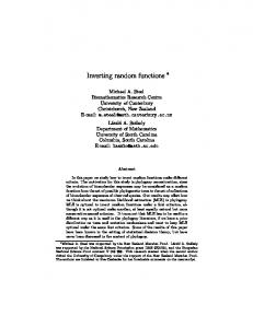
Breed and co-workers have carried out detailed measurements' ' of the magnetic properties of several antiferromagnetic alloys which closely approach the idealized models treated in the preceding sections. They have studied, in particular, KMn~Mg, ~F, and K,Mn~Mg, ~F, . The former is found to be a very isotropic Heisenberg antiferromagnet, with 6„= H„/He&10 ', an—d J= —0.345 meV (4.0 K),' independent of concentration. The magnetic atoms occupy the sites of a simple cubic lattice, and nonmagnetic Mg" ions apparently substitute randomly for the Mn"(S= —,) ions. K, MnF, is accurately described as a 2D square antiferromagnet, the Mn" ions confined to well-separated planes in the crystal structure. Interactions between planes give rise to an anisotropy 5„= 0.004. There is evidence from the Curie-gneiss plots of y(T) at high temperatures that J~ increases with dilution in K, MnPlg, ~F, . Breed et aI. find J/0

'

~

100 {kOe)

150

200

FIG. 12. Magnetic moment per site M, at low temperature as a function of transverse field for dilute (data K2Mn&Mg f pF4 alloys at several concentrations from (Ref. 2). The diamonds are for P =0.74, the circles for P =0.84, and the dots for P =0.93. The solid lines give the corresponding magnetization as calculated numerically, as described in the text, using samples of 80 F80 sites (p =0.74), 60 x60 sites (p =0.84), and 44 x44 sites (p =0.93). The dashed line indicates the magnetization expected for pure K2MnF4. The dotted curve shows the contribution of the isolated clusters included in the calculated magnetization for p =0.74.

"

.

CQ

= —4. 2[1+0.43(1 —p)], and interpret the increase as a result of the discrease in over-all lattice constant upon doping with the smaller Mg ions. The large magnitude of the Mn spin makes the classical treatment of this paper an appropriate first approximation to the properties of these systems.

Calculations"'"" of high-frequency

excitations

substituted Heisenberg magnets, giving detailed agreement with results of neutron scathave appeared elsewhere. In this section tering, we compare the static susceptibility calculated by to check our methods with Breed's measurements, our predictions of the increase of X, on dilution and of the divergence at p, . The experimental data does support our picture of the importance in y, of ferrimagnetic fluctuations, but in a way which was not anticipated. The most obvious feature of the experimental data at low temperatures, plotted in Figs. 12 and 13, is the nonlinear field dependence of the magnetization. In both 2D and 3D, the low-field susceptibility increases with decreasing concentration, while the susceptibility at high fields rein randomly

"

A. BROOKS HARRIS AND SCOTT KIRKPAT RICK

560 0.80

0.60

E

0.40

16

in fields up to 200 kOe at 4. 2 K. We hive done this for clusters containing one to three adjacent Mn atoms, and also for clusters with three spins on one sublattice adjacent to one on the other sublattice. We treat these small clusters since they are the most common, and larger clusters do not have as great a net moment per site at low fiejds. Above = 50 kOe, those clusters with a net moment in zero field are oriented parallel to h, while fields of order 200 kOe begin to overcome the exchange fields, and draw moments of roughly 'S per site even from isolated pairs of spins, —, which have no zero-field moment. For each of the concentrations shown in Figs. 12 and 13, we summed the contributions from these small clusters with appropriate weights. The result is shown as a dotted line for the case of lowest concentration in each figure, and proves to be negligible for the cases in both figures. In all higher-concentration cases, adding this cluster moment to the linear response characteristic of a uniform material fails to account for the observed curvature in M versus „„

CCI

0.20

0.0 100

50

H

150

200

(koe)

FIG. 13. Magnetization as a function of transverse field at low temperature in KMn&Mg& & F3 (data from Ref. 2). The diamonds represent p =0.82, the circles are p =0.58 and the dots are for p =0.39. The solid lines give the calculated magnetizations for these concentrations, including the effects of isolated clusters. Samples sizes used are 24x 24x 24 (p =0.39), 14x 14x 14 (p =0.58), and 8x 8x 8 (p =0.82). The dotted curve gives contribution to the magnetization for p =0.39 obtained by enumeration and exact solution of clusters of four or fewer sites.

mains constant or decreases. The curvature of the plots of M vs H increases with decreasing concentration, and is slightly greater in the highly isotropic 3D alloys shown in Fig. 13 than in the data from the more anisotropic 2D alloys (Fig. 12). Isolated finite clusters of spins play a minor role in the nonlinear field dependence seen in Figs. 12 and 13. To begin with, they are relatively rare. For the 2D case with p =0.74, numerical study shows that only 0. 65'7o of the magnetic sites lie in isolated clusters. For the two higher concentrations, less than one magnetic site in 10 is isolated. For the 3D case with p= 0.39, p —P(p) is found to be =0.047; for p=0. 58 it is =0.007, and for P = 0. 82 it is negligible. It is not difficult to calculate exactly, for clusters of a few spins, the moment induced per site

The ferrimagnetic fluctuations discussed in the previous sections do provide a mechanism for the nonlinear response, and conversely this type of high-field measurement appears toprovide a method for the direct observation of such fluctuations. In the construction of a lower bound to y» (129)—(134), it was found that large contributions to m, came from regions in which the net spin differed from zero by one or more standard deviations. In the presence of a finite external field, the spins in such regions may deviate through angles large enough to cause the small angle approximation made in calculating X, to break down. Thus we argue that the low-field limit of BM/BH in Figs. . 12 and 13 should be identified with X, as calculated in Secs. VI and VII, and that the nonlinearity arises from the gradual saturation of the response of the ferrimagnetic fluctuations. This can be checked quantitatively by examining the microscopic details of a computer simulation similar to those of Sec. VI. First we give an expression for the microscopic energy in the presence of a uniform field h=h, x in a form which makes the angular dependence explicit:

„,

sin8, , e„,= — pi, j p, p, S, S, cos(.8, .+8,) —g, p, S, cos8,. —gp~ p p, S,.h, „, 2

.

~&~

. .

.

.

.

(141)

i

where 8,. is the angle through which S,. relaxes in the x-z plane as in (50). The equilibrium

conditions (44)

become 2

J g p,. S,. S, sin(8,. + 8,) + &, S; sine, . = g .

~

~

.

p, ~

„,

S,.h, cos 8,

In order to derive an efficient iteration procedure to solve (142), we write it as

(142)

RESPONSE FUNCTIONS

16

Q,. =

g

~Z~P&S,. S, (u., v,

SYSTEMS

g— yak, S,. v, =0,

If an approximate

Q, is

5Q,. =

MAGNETIC

„,

)+;S,.u;

+.v, u,.

where u, , v,. denote sin8, , cos8,

OF RANDOM

561

(143)

solution fu, .) is changed by

(«,], the .

,

resulting

P K, ,v, '«, ,

change in

(144}

.

where

K, , =5,,

2

J p~S,. S~ v,.v~ —u,.u„+, -S,-v,. +gp, ~h,

At each iteration, assume that the (u,.] are a reasonable first guess to the solution of (143). For example, the (u,.) might be the correct result for a slightly smaller value of h, . Then a .), such that good choice of Q,. ((u,. + «&]} vanishes to first order in all 5u, , is given by

„,

(«,

«; = —P v;(K

');;Q, ({u,])

One precaution is necessary. any ~u,. ~&1, large increments

The incrementing u'.

To avoid making must be compressed.

formula

""'=u'. "'+ «, (I+ [«,/(I ',

(146)

"'+ «,.f1 + [

i

5u,.

i

—u, )]'].

','

/(I+, .)]'j

5u, &0

',

«,. & 0 (147)

""' remains Q',.

of order 5u' has the property that and ~u,. ~& 1. Using (146) and (147), it was possible to obtain solutions to the nonlinear equations (142), with a maximum error of 10 ' in any of the u,. in two or three iterations, whenever h, ~ 0. 1H~, starting with all angles zero, and for larger values of h, by starting with a solution for a field roughly half as great. The magnetization as a function of field was calculated by this procedure for each of the experimental concentrations, using the parameters given in Ref. 2. The contribution of isolated clusters was added where significant, and the results are given by the solid lines in Figs. 12 and 13. Theory and experiment agree to well within the uncertainty in Breed's determination of J for the cases p = 0. 74 and p = 0. 84 in. Fig. 12. We have no explanation for the discrepancy at high fields between the theory and the experimental points for P =0.93. Since the data points lie below the response expected for pure K, MnF, (the dashed line), the cause must lie outside of the mechanisms discussed in this section. The data on the 3D system KMn~Mg, ~F, (Fig. 13} also agree well with the calculations. Agreement could be improved by performing the numerical calculations on larger samples, since this would

„,

„,

„,

S,-N,. +2

Z

p,. S,. S,. v&v,. —n,.u,

improve the treatment of fluctuations of large spatial extent, and thus enhance the magnetization at low fields without increasing it greatly at higher fields. One might also extend the calculations of finite-cluster contributions for the case p = 0.39. Since a rough calculation suggests that the dotted line in Fig. 13 represents at least 3 of the isolated-cluster moment, and exact solution of much larger clusters is prohibitively difficult, we did not attempt this. It seems valid to conclude from Figs. 12 and 13 that ferrimagnetic fluctuations do account for the unusual observed magnetization, and that this sort of nonlinear susceptibility may be considered indicative of an inhomogeneous response on the atomic scale. Figures 14-16 provide a microscopic examination of the fluctuations. In Fig. 14 we show the distribution of values of sin8,. observed in the 30 simulations at three concentrations, in each case using h, = 30 kOe. The distributions extend to negative deviations in all cases. The distribution broadens as the concentration is decreased, and the rate at which it broadens exceeds the rate at which the average spin deviation increases. In contrast to Fig. 14, the distribution of cos(8,. —8,.), which determines the exchange energy associated with each bond, is found to remain sharp until much higher fields. Thus the two sublattice moments remain nearly opposite everywhere, but the moment in regions where one sublattice dominates can swing into the fieldby appreciable angles. The snapshots of equilibrium spin orientations shown in Figs. 15 and 16 confirm this picture. Figure 15 shows a single layer of a 3D sample with p in the vicinity of p, . In the smallest fields applied [Fig. 15(a)], the local orientation of the sublattice magnetzation swings through angles of up to 45 . [The field applied in Fig. 15(a) is roughly 2800 Oe, if we use parameters appropriate to KMnF, .] Doubling the field [Fig. 15(b}] produces only slight increases in this over-all relaxation. In both Figs. 15(a) and 15(b), neighboring spins remain very nearly antiparallel throughout. Another fourfold increase in h, [Fig. 15(c)] be-

„,

„,

A. BROOKS HARRIS AND SCOTT KIRKPATRICK

562

16

gins to draw the two sublattices out of alignment

K Mn

locally. The local relaxation decreases rapidly with increasing concentration. Figure 16(a) shows the effect of applying the same field to a p=0. 55 sample as was applied in Fig. 15(a) to a more dilute sample. Deviations from the easy axis are less than 10' everywhere. Applying a field h, = 0.067H~, as shown in Fig. 16(b), produces spin deviations comparable tothose shown in Figs. 15(a) and 15(b). In the terms of the preceding section [e.g. , (139)], this suggests that L(0.40) is from four to eight times as great as L(0.55). Finally, application of a large field to the sample [Fig. 16(c)] produces large local deviations between the two sublattices. [Using KMnF, parameters, h, in Fig. 16(c) is of order 120 kOe. ] The microscopic phenomena seen in Figs. 14-16 should be experimentally accessible. Experiments such as nuclear magnetic resonance or Mossbauer effect, which probe the induced hyperfine field at a nonmagnetic impurity site, will measure the net moment of the neighboring magnetic ions. In a these ions may sufficiently dilute antiferromagnet, relax almost independently, even though they may be separated by only a few lattice sites, as occurs at the circled sites in Fig. 15. Thus the ferrimagnetic fluctuations will cause a field-dependent broadening of the observed hyperfine fields. A more direct and easily interpreted measurement is neutron diffraction to measure the static susceptibility at finite wave vector. This is given

F3

Mg1

„,

= 30kOe

H

p

„,

=.79

45

-1.00

-0.50

0.50

0.0

by

1.00

sin(8;)

X' (q, o}

FIG. 14. Distribution of transverse spin deviations (sino; is plotted) in an applied field of 30 kOe for The calculations are KMn&Mg& & F3 for three dilutions. based on (142) and were carried out for samples similar to those used in Fig. 13. .

/

t

0/

s

toi

Oi

Q

~O/

s

/

s

s

t

/Q.

t

so / /

t

I

(146)

I

it5y i ~ Or

r0

//

I

Or

rl

P

/

r

Qr

~Q/

t

/0

I

rp

I

t

t

t-s

I

t

00 t

I

t

//

/Q//

t

ir

t

I

t ItItS tt

= 0.4

hext

= 0-008 HE

s&ts/

orx

/

//o OQii

GO t

I

.

t

s

00

(b)

s

t

IQ~o 0

I

/Q

0 O~~-

t

t

I

/0

/

s

t

tttsIO

ohio

/

rQ~~.

t

s

P

I

I

t

so

(a)

I

/

O

OQ

t&t t&'iy tIO&

s+)o s

(r —r')]drdr',

/

. / .

/

(r}.m, (r'}}

where m, ( r ) denotes the component of m( r ) perpendicular to q. We now consider an experiment

/ /

(m,

x exp[i'

/

s I

f

/

s

t

y

O

t

&

p

= 0.4

hext

(c) P =04

= 0.017 HE

hext=00

E

FIG. 15. Equilibrium orientations of the spins in one layer of a randomly diluted 3D (20& 20& 20 site) antiferromagnet with a concentration of 0.40 and transverse applied fields (a) h, /H~ =0.008, (b) /H~= 0.017, and (c) h, /H~ =0.067. Some nonmagnetic sites at which the hyperfine field broadening described in the text would be observed are circled.

„,

h„,

„,

RESPONSE FUNCTIONS

16

t

I

~

It

I

I

tttI tt

I

I

tie

t

I

t

~

t

~

t

t

t

t

t

~

»

tt

fI tI

~

~

t

I

II

t -

(a)

p

I

~

- 0.55

j

/'

FIG. 16. Equilibrium spin as in Fig. 15, but for one layer in a 14 x14x 14 sample with concentration=0. 55 and h, /Hz =0.008 in (a), =0.067 in (b), and=0. 33 in (c).

~

~

orientations

~

„,

~

~

~

I

tent t

+

&tl h~t

)

~

/

t

I ~

/

t

I

t

~

SYSTEMS

MAGNETIC

OF RANDOM

&

i

I

~

~

~

j

I

he„t= 0.008 HE

(b) p = 0.55

he« = 0.067

HE

q lies along the easy axis and a field is applied perpendicular to q. In a pure system, the only magnetic contribution to the elastic scattering will be a small additional amplitude of the ferromagnetic Bragg peaks. In contrast, in the random system, as illustrated in Figs. 15 and 16, the staggered magnetization is pulled away from the easy axis in the ferrimagnetic regions. Thus, locally one obtains a staggered magnetization perpendicular to q. This local order persists over distances which are governed by the connectivity of the dilute network. Accordingly, the field-induced superlattice reflections will have a width proportional to f ', where f is the physical distance between nodes introduced in Sec. VIII. Thus $ can be measured by neutron diffraction.

for which

X. RESULTS FOR GARNETS In this section we present numerical results' for randomly diluted or mixed garnets. Per unit cell, all the garnets which we will consider can be represented by the formula

41[Fe, „M„][Fe, ,M, ][R, , S,]o»],

(149)

where M represents one or more trivalent nonmagnetic ions substituted for the iron ions and 8 and S are both trivalent rare earths, or one may be yttrium. The grouping of ions in square brackets in (149) indicates the relative occupation within the a, d, and c sublattices. Pure YIG is described by x = y = z = 0 with 8, being yttrium, which is nonmagnetic. The systems described by (149) can be prepared over almost the entire range of Nonmagnetic the parameters x, y, and z. alkaline-earth ions are also commonly. substituted for Y in order to reduce the net lattice constant changes when the Fe ions are replaced by ions of very different size. Since this introduces no new magnetic phenomena, we shall ignore this possibility. We will first present results for diluted YIG where A = Y and x=0. Subsequently, we treat rare-earth garnets in which B and 8 are magnetic. For dilute YIG we show in Fig. 17 the percolation

'" "

(c)

p =

0.55

hext

- 0.333 HE

threshold as a function of the fraction of vacancies on the d (majority) sublattice. The threshold occurs at the highest net Fe concentrations when substitution is confined to a single sublattice. That is, Fig. 17 shows that to disconnect the system requires the removal of 1.6 of the two Fe ions on the a sublattice, leaving a net Fe concentration of 68 at. %, or 2. 6 out of 8 Fe ions on the d sublattice, leaving 48 at. /o. For substitution of nonmagnetic ions into Fe sites with no preference for either sublattice the critical Fe concentration is 40 at. %. Thus, we conclude that subsititution confined to a single sublattice produces more drastic effects than completely random substitution. We next show, in Figs. 18-21, A as a function of composition for various types of dilution in that J~~/J, YIG. It is believed" J„/J«=0. 1. In Fig. 18, we show that the effect of including the second-neighbor interaction J~„onA(x, y)/A(2, 8)

""

j

&

j

&

/

I

[

„=

I

PERCOLATION

2- x 3-y

~ 40 &

j

I

f

I

/

I

I

/

[

I

THRESHOLDS

$+

x+y

l2

o

Z.

o 2.0 I.O

0

t

0

l.

":~. 0.2

0.4

f (FRACTION OF VACANCIES

06

08

ON MAJORITY

I.O

SITES)

FIG, 17. Percolation threshold for the dilute garnet system. The vacancy concentration is 2 x on a sites and =y/(x+y) is the fraction of the 3y on d sites, while vacancies which are on the d sublattice. The shaded areas represent the number of sites (per formula unit) occupied at threshold on the majority (d) or minority (a) sublattice.

f

A. BROOKS HARRIS AND SCOTT KIRKPATRICK

564 I.O

0.8—

[Yz-xcex]Fee[Fe~ xsix]o~z

0.6— J =oi~

(Jdd =O. Jaa

X

I

d,

&

0.4—

(Jdd Jaa

"

=0)

0, 2—

0.0

2.50 3.00 2.00 5 X FIG. 18. A(y) vs 3-y for YIG diluted only on the majority sublattice. The circles were calculated under the approximation Jzz =0, while the triangles show interthe effect of introducing next-nearest-neighbor actions (Jqq/~ad =0, 1, ' aa ). Calculations in this and the following four figures were made on samples with 7000 Fe sites.

00

0, 50

1.

I.

50

J„=

is quite small in the case where substitution occurs on the majority sublattice only. This is the case in which the effect of J«should be slightest, since every d sublattice ion remaining has a full complement of a sublattice neighbors. The effect remains small for small dilution even when equal fractions of the Fe sites on the two sublattices are 1.00

„Fe3

Y3 Fe2

0.80

y

Mx+

substituted, the case depicted in Fig. 19. J«affects the stiffness in a more drastic way by causing the Neel state to be unstable whenever a d ion has no a neighbors. This occurred whenever g+y &1 in the case of Fig. 19, and at all concentrations considered for substitution on the minority sublattice only, shown in Fig. 20. This observation is consistent with the suggestions of Rosencwaig" and Geller, that random canting takes place on the sublattice with the smaller number of vacancies. Since this presumably affects only a small number of sites, and the effect of J«was found to be small until the instability occurs, we have taken J«= J„=Oin the cases shown in Figs. 19-21, and do not attempt to model any random canting. Also shown in Figs. 19—21 is the behavior of the spin-wave stiffness D, calculated by D(x) eeA(x)/ M(x), where PI(x) is obtained by taking the Neel state magnetization for spins in the infinite cluster. In Fig. 21 we have used the actual 90% dsublattice preference found" for Qa substitution of 30% or less. Since the magnetization passes through zero at a compensation point in this case, D increases with dilution, and changes sign. (The absolute value of D is plotted in Fig. 21.) The behavior of the spectrum at long wavelengths close to such a compensation point is studied in more detail below. These calculations of A(x) for Ga substitution may be compared with available measurements of spinwave resonance at room temperature. In making

"

this comparison it is important to realize that T, also depends on Fe concentration, and that this is

012

1.00

= 3x/2

Y3 Fe2-x Fe3 Mx ~ D(x, y)/D(2,

0

0.80

3)

A(x, y)/A(2, 3)

0.40

~ D(x, 3)/D(2,

0 0.20

1.50

3)

0

A(x, 3)/A(2, 3)

0.40

0 n

0.0

012

0 I

0

I

2 00

2 50 5

I

3 00

I

3.50

—x —y (Fe atoms/formula

I

4 00

0.20 4 50

5

00

0

unit)

()

FIG. 19. Exchange stiffness A(x, y) for YIG, plotted as a function of total Fe concentration, for the case when dilution occurs with equal probability on the two sublattices. Only nearest-neighbor interactions (J, were included. The spin-wave stiffness, D(x, y), is indicated

„)

by the solid data points.

o

~

~

0.0

0.50

0.75

1.00

1.25

) —x (Fe atoms/formula

1.50

1.75

2.00

unit)

FIG. 20. A(x) and D (x) vs 2-x as in Fig. 19, but for dilution on the minority sublattice only.

RESPONSE FUNCTIONS

16 2.00

SYSTEMS

MAGNETIC

OF RANDOM 1.00

Y3 Fe2 x Fe3 y Gax+

012

~& ~ p

0.80

8

g 0.60

1.50 ~ D(x, y)/D(2,

3)

& A(x, y)/A(2,

3)

p

4p

leap

g

~q

p

0

~~ p

0.40 ~ ~ ~ ~

p

p

Q

0.20

1.00

~+

t

~

lt

p

p

0.0 0.0

0.40

0.20

0.80

0.60

1.00

b (fraction of bonds present)

FIG. 22. Exchange stiffness A (data of Figs. 18-21) plotted versus b, the fraction of bonds which are present. The cases plotted are doping on the minority sublattice only (circles), doping with the same probability on both sublattices (diamonds), Ga substitution (squares), and dilution of the majority sublattice only (points).

0.50

0.0 2.50

3.00

3.50 5

00:

4.

—x —y (Fe atoms/formula

4.50

5.00

unit)

FIG. 21. A and D versus total Fe concentration as in Fig. 19, but for y/x =8, the ratio applicable to most Gadoped YIG samples at moderate vacancy concentrations (Ref. 69).

while it is a nonlinear function of site occupation when both sublattices are substituted, as Fig. 19

demonstrates. Finally, the behavior of A(x, y) for nearly pure YIG can be understood qualitatively using the results for cubic systems. We use the result, based on the approximation (91) that

"

the dominant source of composition dependence in the value of A at room temperature. The theory of Ref. 45 can be improved by using the zerotemperature dependence of A on concentration from our numerical work, as is described in Ref. 9, and very close agreement is achieved. However, no existing theory can explain the unusual temperaturedependences reportedby Enoch et ajt. Our result for A(x, y) are usefully summarized by the approximate empirical formula

"

A(x, y)/A(2, 3) = 1 —0. 73x

(152) when nonmagnetic ions are substituted without preference for either sublattice. For the garnet lattice a=6 for g sites and 4 for d sites. Therefore, (A 'dA/dc —2} is expected tobe slightlylarger for garnets than for the sc lattice. To estimate it for garnets, we assume that (A 'dA/dc —2) is proportional to (z —1) ' and scale the sc result accordingly, using z-5 for the garnets:

0.43y+ 0.25xy, (150)

are plotted in Fig. 22 vs b, the fraction of bonds which are present:

dc

and

4

"

sc

dc

2

-2

66

(153)

Our results, as summarized in (150), yield A ' dA/ dx-0. 73, and A. ' dA/dy 0.43 in the low-dilution limit. Thus, for —,'x+ —,' y=c we obtain A 'dA/dc =2. V, in agreement with our theoretical estimate. It has been suggested on empirical grounds" that the variation of T, with dilution can be related to that of A by

-

= 1 —pg —31 g+

6gg.

(151)

Since the coefficients of x, y, and xy in (150} are in nearly the same ratios as in (151), the points in Fig. 22 fall close to a universal curve. In contrast, if the data of Figs. 18-21 are plotted versus the fraction of missing sites, four distinct curves result. In Fig. 22 we also observe that A(x, y) varies nearly linearly. with bond concentration,

"

T,(x, y) /T, (2, 3) = A(x, y) /A(2, 3),

(154)

stiffness. As we where A is the zero-temperature have seen in Table II, this relation does not hold

A. BROOKS HARRIS AND SCOTT KIRKPATRICK

566

700

600—

20

„] „] „Ca„] „Si„]0)2

&-()) Y3 [Mg„Fe2

l6

[Fe3 „S(„]0~2 Fe3 0)2

o-(2) Y3 [Sc„Fe2 ~ -(3) [Y3 Fe2 [Fe3

lo— oE

500

q, a

5

0-

400

+ ~00

-IO

0.05

I

I

0.20

0.15

O. IO

FIG. 25. Dispersion relations for the acoustic and lowenergy optical mode for Si-doped YIG near compensation where q, is defined as calculated from (32). For in (36), the frequencies vary as q; for q» q, they vary

200 I

I

I

q«q,

00

as q.

0 0

2.0

I.O

5.0

FIG. 23. Comparison of the measured (Ref. 4) T~ fear three substituted YIG series and the values T, would take (solid lines) if it were proportional to A. even qualitatively for simple lattices. For the garnets this relation is more reasonable, but still is not satisfactory, as can be seen from Fig. 23, where we compare experimental values of T,(x, y) T, (2, 3) with our numerical results for A(x, y)/ A(2, 3). Clearly, it would be useful to have experimental values of the latter quantity to corroborate our calculations. The lowest-energy long-wavelength modes in diluted YIQ can be treated by the continuum approximation (32), which predicts two modes. Of particular interest is the case when dilution occurs predominantly on the d sublattice, so that The two effects of M(x) =M~(x) —M, (x)- 0. dilution we wish to illustrate are (i) as M(x) -0, the frequency of the optical (exchange) mode vanishes, and (ii) when M(x)-0 the dispersion relation shows both vccq and zv ccq' regimes. To

""

j

study the optical-mode frequency we have calculated X, and M for dilution only on the d sublattice, as is thought to occur in Si substitution. Compensation occurs at T=0 when y= 1, since M (y) -(1 3 y)M„(1)this far abovethepercolationthreshold. The predicted &u„,(y) is plotted in Fig. 24. The curve is asymmetric about y= 1 because )(,(y) increases more rapidly below y = 1 than above. At compensation, X,(y) 1)(,(0). To exhibit the changeover in ur from linear to quadratic depen-10 cm '. dence on q, we study a case in which This will occur for y-1. 95 or 2. 05, and is plotted in Fig. 25. For either choice of composition, crossover should be observed at q, a- 0.08. We next -consider mixed rare-earth iron garnets. Here a simple two-sublattice model can again be used, at low energies, since the Fe-Fe exchange interactions are much stronger than the Fe-R terms. In this model we treat only excitations in which all iron spins precess nearly in phase. Likewise, all rare-earth spins are considered to precess in concert. There will also be excitations in which rare-earth spins are incoherently excited at the single-ion frequency, , given by"'"

-1.

~„,

v„.

hu„.=I4Z,

E

500

where S~, = J~, and

200-

couplings. 0

IOO-

0 0 0

0

0

0

0

0

l. o

2.0 3 —g

FIG. 24. Optical-mode frequency for Si-doped YIG (dilution only on the d sublattice) calculated from (33) using Monte Carlo data for X ~ and M& -M, .

4„.S, ,

(155)

is the iron spin and we assume that

J„areboth

0

0

&

—BZ„ISF,=

negative (antiferromagnetic)

In a garnet containing two species of rare-earth ions having sufficiently different values of co„.we expect to find two bands of incoherent single-ion excitations. The energies we are considering are low enough that only the lowest acoustic mode of YIG, shown in Fig. 26(c), will be relevant to alloys of YIG with rare-earth ions. Tinkham' has treated excitations in pure YblG in this spirit. His approach leads to a 2 by 2 secular determinant, with exchange terms &„. SF, or coupling the Yb and Fe sublattices. Since

4„S~

i6

RESPONSE RUNCTIONS

J,, and J„arenegligible

in comparison

with

OF RANDOM

„,

1

—&„Dvzoq' = 0,

S„

v„at

(u

= —Dq~ = —Drzoq~(Sq —S )/(Sq

S, S ),

(15V)

"

and has the correct dependence on total spin given by (13b) and (14), as has been noted previously. For S, —S, &0, D is positive and an acoustic spin wave tends to decrease S,. This is the case in YIG or YbIG, shown in Fig. 26. For —S, —S, &0, D is negative and an acoustic spin occurs in GdIG wave tends to increase

S„-

S„—

S„

S„-S„as

(Fig. 26).

The optical mode at q =0 is given by (156) as Gd

IG

Yb

IG

(158)

We can now make contact with Tinkham's work, which reproduces the original formula of Kaplan for a two-sublattice system, viz. and Kittel'

'

(u,

t= X(y, M~ —y~M, ),

(159)

where A. is an exchange constant and y, and M& are the gyromagnetic ratio and magnetization of the ith sublattice. This notation makes it appear that co depends on y, However, as we have previously noted, ~ is independent of the g values. We can rewrite (33) in the form, -

h&u„„=p, ~s(S~ —S, —S,)/(y,"v,),

(160)

" y, is

the spin-spin susceptibility defined in where I as the susceptibility evaluated for unit g values, and v, is the volume of the unit cell containing 12 d sites. One can show that y, is

"

—S,)/(h(uszvo),

Xz' = Pzz(Sq

(161)

which shows that (160) and (158) are equivalent. We now present some results for mixed rareearth-iron garnets. We assume that all the iron sites are occupied and characterize the rare-earth sublattice by its spin density S,. For YbIG, =27.8 cm ', 0 cm ', and for GdIG, S+„=25. so the approximation of treating the two types of rare-earth ions as a single sublattice should be reasonably good in (Yb-Gd)IG. As S, —S, —S, is decreased, for example, by

"'"

"'"S+„.

l

S~„,

l

becomes small. The appropriate dilution, evolution of the spin-wave spectrum versus concentration for mixed (Yb-Gd)IG is shown in Fig. 27. In this connection it is interesting to note that does not imply the zero-spin condition S, =S„-S,

YIG

qa

(c)

(b)

20E

567

S, —S,)/(S~ —S,) . hv„,= h&u„.(S„—

(156)

where S„andS, are the spin per unit cell on the d, a, and c sublattices, respectively. = 12(— ', = 30, S, = 8(-,') = 20, and for GdIG ) S, = 12(—,) =42. For YbIG, S, =6, since the Yb" ions is in a Kramers doublet" with S,«= &. The two branches obtained using (156) for GdIG and YbIG are shown in Figs. 26(a) and 26(b). For completeness we have also indicated the presence of incoherent excitations of the rare-earth spins at frequency Equation (156) is the analog of (32) if the definition of y given in (14) is used. The only difference between (156) and (32) is that in the former a term —cuD~, Gq' is included. This term is unimportant in the hydrodynamic regime, but insures that one root of (156) will tend to large q. For small q the acoustic mode obtained from (156) is

S„,

SYSTEMS

J,

is the same as in pure YIG, and a stiffness term D~«q' appears in the Fe-Fe element of the secular determinant. The secular equation can be written

A

—&[& z(Sq —S —S )/(Sq —S ) —Dvzoq

MAGNETIC

(d),

z

(e)

-l00 I

qo

-200

I.O

q0

I.O

lO

E

-20-

-300

-40

-50

FIG. 26. The low-energy region of the spin-wave spectrum of various pure garnets. The incoherent excitations on the rare-earth sublattice (in GdIG 'and YbIG) give rise to a spin-wave band centered at the single-ion The other modes in GdIG and exchange energy, YbIG, arising from the coupled motion of the two sublattices, have frequencies determined by (156). For YIG, this model yields a single spin-wave branch whose dispersion is given by (157) with S, =O.

4„.

FIG. 2V. Low-energy regions of the spin-wave . spectrum for some mixed garnets, with the formula [Yb„Gdg „]3Fe&Off in panels a-d and for pure YIG in panel e. In case c, spin compensation occurs, and for ~ q. The optical mode, whose both acoustic branches frequency at q =0 is given by (158), is indicated by an arrow.

A. BROOKS HARRIS A5 8 SCOTT KIRKPATRICK zero magnetization, since the g values of the rareearth ions are not equal to the g value of iron. Indeed, pure YbIG is an antiferromagnet in the sense that its magnetization is very nearly zero at T=O. However, its spin-wave spectrum is ferromagnetic with a single acoustic modewith v, o-q' [Fig. 2'7(d)]. ' By contrast, Fe, (Gd, Yb, ,),0», withe =-, has zeroeffective spin, and therefore an antiferromagnetic spectrum in the sense that the acoustic mode is twofold degenerate and has ~, ~q [Fig. 27(c)], but has nonzero magnetization. In this case, for small q, i. e. , for Dq'&A~„. one has

hv,

,Da'q'. —

= + (h(o„D)'~'aq —

(162)

particularly interesting question is raised by the possible occurrence of well-defined optical modes in such mixed systems. Are these optical modes well defined at all concentrations, or is our continuum treatment restricted to certain ranges of concentration? The clearest answer to this question will probably come from experiment, since these modes are observable by infrared spectroscopy. A

"*"

XI. SUMMARY AND CONCLUSIONS

(i) In the limit of small anisotropy, the hydrodynamic picture of spin waves first introduced by Halperin and Hohenberg" gives useful predictions for disordered ferromagnets, ferrirnagnets, and The frequencies of the eleantiferromagnets. mentary excitations at long wavelengths and low energies are given by

(12)

+ DQ'

for ferro- and ferrimagnets, co

=coo+C

and by

g

for antiferromagnets, where D and C are related to the static magnetic elastic constants A, the exthe perpendicular susceptichange stiffness, bility, and M, the average magnetization per unit volume, by D= 2'/Mand C'= 2y'4/g~, where yis the gyromagnetic ratio. In this paper, we have evaluated A, X„andM for various random dilute magnets at arbitrary defect concentrations. The elastic constants were then used in the hydrodynamic framework or extensions thereof to discuss elementary excitations. We have confined our examples to dilute systems in this paper because these are the most difficult for conventional "average-medium" theories to treat. Applicability of these methods to a twocomponent antiferromagnetic alloy has also been demonstrated in a previous paper. (ii) We have carried out an exact calculation of the effects of a single defect in order to estimate the

y„

""

"

errors resulting from the use in (12) and (18) of the hydrodynamic expressions for D and C (in terms of static elastic constants) when the gap frequency leads to U se of the static parameters 40p ls finite. errors in the gap frequency and in (d&u/dq'), of order &u, /~z, where &u~ is the exchange frequency. (iii) For high concentrations of defects, for more elaborate types of disorder, or for materials with complex crystal structures, the magnetic elastic constants can be obtained numerically by a simulation method. We have calculated M(p), A(p), and, for antiferromagnets, y, (p), for the planarsquare, simple cubic, body-centered-cubic, and garnet lattices. These calculations reproduce the results of the single defect theory as p I, except in the case of garnets, for which no single defect results are available. (iv) The static elastic constants display critical behavior near the critical concentration for percolation. We have obtained estimates of the exponents characterizing this region for the square and simple cubic lattices. Inequalities relating these exponents to the exponents occurring in the more conventional percolation cluster statistics problem have also been obtained. The critical dimensionality for the onset of mean-field behavior in the elastic constants is found to be 6, as is also true for the static cluster properties. (v) We have shown that configurational fluctuations cause X, in an isotropic antiferromagnet to diverge (i) as p-p„and (ii) in two or fewer spatial dimensions for all P41. In both cases the diver gence results f rom local fluctuations in the total spin which are present because the two sublattices in a randomly diluted antiferroAnisomagnet are not balanced microscopically. tropy removes the divergence in both cases, but a prominent maximum in X, persists at x, . As a consequence of the type (ii) divergence, &u~q/ (lnq)' ' as q-0 in an isotropic two-dimensional dilute antiferromagnet. (vi) We propose two experiments in antiferromagnets to observe conf igurntion fluctuation which give rise to locally f err omagnetic regions. The induced hyperfine field at the nucleus of anonmagnetie impurity will be broadened by the application of a transverse magnetic field. Elastic neutron scattering in the presence of a transverse field can sense the magnitude and length scale of these fluctuations. (vii) We have studied the nonlinear response of dilute antif errom3gnets to an external f ield perpendicular to the easy axis. This calculation reproduces the field-dependence seenby Breed et aE. ' in dilute 2D and 3D systems. The principal cause of the nonlinearity is a breakdown of the usual small-angle approximation which occurs when the ferrimag-

,

-

y„

""

RESPONSE RUNCTIONS

16

MAGNETIC

OF RANDOM

netic fluctuations approach saturation. (viii) Dilution of aferr imagnet predominantly on its majority sublattice can create an antiferromagnet. The crossover from ferri- to antiferromagnetic behavior can be studied in a continuum approximation which is a natural extension of (12} and (18). At concentrations close to the compensation point there exists a spin-wave optical mode whose frequency is proprotional to the unbalanced spin density. For dilute YIG the variation of the optical mode frequency with dilution, shown in Fig. 24, should be observable by infrared absorption measurements of the type done by Sievers and Tinkham" on pure YbIG. We also propose study of dilute JYb-Gd)IG to explore the details of this crossover (see Fig. 27}. These alloys have the interesting feature that angular momentum compensation occurs at a different Yb concentration than does magnetization compensation. Thus one can study a system whose elementary excitations resemble those of an antiferromagnet, but which has an appreciable net magnetic moment.

~

gn)

~

569

~(n) ~(n)

J

j

SYSTEMS

(A1)

where

X„.=p,. Q(6, , p, , „-&,, „p,),

(A2)

.

d

where d is summed over nearest neighbors of i. The matrix N is a conductance matrix because it has the properties

¹,

N],. =0,

(A3a)

=N,.;

(A3b)

~

Note that there are eigenvector(s) corresponding to &'" = 0 which involve solutions x" uniform over a cluster. The uniform solution oyer the infinite cluster is denoted

g':

N'"

(jC ),

(A4a)

~(o)

(A4b)

0

"

@here X is the number of sites in the infinite cluster. According to Brenig, there are solutions

ACKNOWLEDGMENTS

The authors gratefully acknowledge useful discussions with B. I. Halperin, T. C. Lubensky, and W. P. Wolf.

with eigenvalues ~" which we may write in where k is a the low-frequency limit as x+, momentum vector of the first Brillouin zone and

+',

~(k) =aa'u'. The dispersion constant D is related to the conductivity p of the randomly diluted network by

APPENDIX A: MICROSCOPIC DERIVATION OF LONG-WAVELENGTH BEHAVIOR

Sec. III we gave a continuum derivation of the formula for the frequency of long-wavelength spin In

waves in terms of static response functions. That formulation coincides with the hydrodynamic treatment, and therefore should give correctly the frequencies of hydrodynamic or first spin waves. This regime is characterized by ~g«1, where y is a thermal. relaxation time. However, since as the temperature g goes to zero, one z enters the opposite regime, ~v» 1, for fixed ~ as Then the elementary excitations are mey chanical or zero-spin waves, our terminology being analogous to that of zero and first sound in a phonon gas. In this appendix we study the zerotemperature excitations from a microscopic point of view, and obtain results which agree with the This equivalence is hydrodynamic formulation. expected to obtain only in the zero-temperature

-~ -0.

limit. We will discuss the dilute ferri- and antiferromagnets by relating their microscopic equations of motion to those of the ferromagnet, and thereby make contact with the analysis of Brenig et g). They studied the random system

"

D

0

Dpure

&pure

2~1

Q

r'

(A6)

Pr

where here and below p,. is 1 if j G ~, and is zero otherwise. Here the subscript pure indicates the value for the pure system. It is easy to show that where A is the exchange stiffness o/g, „„=A/Ap„„, introduced in Sec. III. Also, if there is no canting, Q,. p,. =M(p)/M(1), in which oase (A6) is equivalent

to (13b).

Now we apply these ideas to the ferrimagnet. Here the equations of motion are

gN$, . =

2 J)~$~ $)

—2

J,) $) $q.

(A7)

We will work at g = 0 and neglect spin-wave interactions. Then $',. =+S„the sign depending on the sign of $,'. in the Neel state. For the random ferrimagnet (or ferromagnet) we set J, , =0 if either site i or site is vacant, and we use (A7) only for spins in the infinite cluster. We write (A7) as

j

h(dS", =

where

pj M;,

S', ,

(A8)

A. BROOK'S HARRIS AND SCOTT KIRKPATRICK

570

J;

M,-,. = Note that M

S

5, , -

-J;,. S';.

is not symmetric

(A9)

and can not yet be

identified as the conductance matrix of a random network. We denote the eigenvectors of M by

where N=

(y„lis

Q

(A10a) ((fan„

I

I

(A10b)

Note that (q is not the transpose of lg„& because In particular, we have M is not symmetric. I

(All)

. „(y„l

(A18)

l(p„&A.

In particular, Ipo&,

M = h(u„(g„.

the transpose of lq„&. Also we have

Nitro&=0 with

(A19)

=P

From Eq. (A15) we see that M= NS

(A20)

where

S],. = 5, , S) .

(A21)

Using (A18) and (A20) we obtain

so that if

PM, , I(„&,=Au„lg„&;,

(A12a, )

M=

+ le„&A„((p„l '. 8

Thus the eigenvalue

then

(A22)

condition for the spin-wave

energies is

g

. m, , (s',. /s', .) q„&,= a~„lq„&, I

(A12b)

or

g iy.».

(A12c)

(A23)

on the left by (qr„l, we obtain

Multiplying . )-'Iq„&, gw, , l(s;)-'lq„&,] =@~„(s',

"l(,&=@~"'l0;&.

&q. ls

(A24) ~, &q, ls 'l 0, & =@~"(q, 0, & Now in the limit A. Brenig et p). find that q becomes a good quantum number, and therefore we may label the eigenvectors and eigenvalues by momentum q and write

"

I

„-O,

Thus &q„I,. =

I

(A13a)

. /s;. q„&,

=lq. &, =0

(if-).

(A13b)

(A25)

. and (g„l, . are the ith components of the Here I(„&, vectors I(„&and (g„l. We normalize lq„& by

&(.I(.&=+1

(A14a)

2 u, (ls.

(A14b)

or &,

)'/S,* =+1.

The q=0 (i.e. , uniform) eigenvector is found using Eq. (A9) to be (A15a) (A15b)

(A26)

Here D and D* and the spin-wave dispersion constants for the original system described by M and that for the modified system described by N, respectively. Brenig et al. 's formulation for the ferromagnet enables us to determine D*. It remains to relate D to D~. This is done by using (A24):

D*(0,IS

(A27)

Now we take the limit

D=D*&q olS

q-0

and obtain

Using (A15) and (A19) we evaluate

To relate the spin-wave problem to a network we define (A16)

satisfies Eq. (A3) and is therefore a conductance matrix. If the eigenvectors of N are lq„&, Now N

then we may write

(A17a)

&q. IN= &q. l~.

(A17b)

&

this as

g p, s, . . '.

(A29)

Finally we relate D* to the stiffness (or conductivity) g of the lattice governed by N according to (A6):

A* Z, I

lp, = x, lg, &

N

(A28)

'lyo&/&q olqo&.

(A30)

Dp*„„Ap„„g, P, Here &* is the stiffness corresponding

to N,

i. e. ,

RESPONSE RUNGTIONS

16

it is proportional to the conductivity of the network described in {46). A" is also the exchange stiffness for the original system described by (A7). Combining (A29) and (A30) we obtain the desired relation

o(()/D(() =(~'() )/~'(())

(g

s ((

g );&;())).

case as mS,', =

Q

J()

S(', +

k

Q

J, ),S))'(, ,

(A32a)

o.

S

g

(A38)

=( S)-'6„.

(A39a) k

k

(A39b) We now proceed as for the ferrimagnet.

We

set I

Ql0. ». &(.

T=

(A40)

I

we rewrite (A38)

Using this expression,

)'n+@~.)ply,

&q. I{@~.

&

= ~.&y.

I

v.

as (A41)

&

in analogy with (A24). Following Brenig ei al we write

r,. )(1+ A,. q)p, , ly, = exp(i q r, ) (1+ 8, q+ C, S &u, )p,

Z'J&)S(

n

l

= exp(iq

&

j

I

&

&

{A33)

„.

where g,. is the number of nearest neighbors of Inserting this into (A32a) we obtain Jz,.

=+„J.

S+ia g+ i S+ia

efjkeJgi kg

Sip

=

where D* is the dispersion constant for the random network described by T. The form (A42a) was previously given by Brenig e] al. , and (A42b) follows in a similar way, except that an additional term of order co, o- q is permitted in Substituting these expresthe antiferromagnet. sions into (A41) we obtain

D*a'q'=

(h(u,

)'Q '

~

(

),('

g (1+X~i

(A34)

~

~

)

g ")

t()(p,. —

x (1+ B,. ~ q + Q)h((), ) ) 1

(A42b)

(A42c)

.

We write this as

S,',

,

,//A=D*a q,

(d+ 88k

~1k

(A42a)

~

~

l

Here S,.', and S,.', denote spin operators for the sites i (on the a sublattice) and (on the I) sublattice), respectively, (d denotes jr ~/2S, and we absorb the sign of J, letting J, denote J, I. To identify these equations with those of a network we eliminate S,.'b:

p

(A37)

(dp]Icp& = Tl(p&,

„.

l(I), &

j:

.

k

Q~))

~S/b

,

at ~ = 0. Equation

where now T is to be evaluated (A37) is of the form [(h u))'a+A

S;.

P T,,S,'.

=

where

571

2,".+(K(a)(); —Q ')

(R~)'Q

(A31) where S,'. (1) denotes the value of S,'. in the Neel state of the pure system and S,'. (p) is the value of S,*. at equilibrium for the dilute system. From the discussion following (A16), it is clear that S',. (p) will only differ from S,'. (1) if there exist clusters coupled to the infinite cluster by competing interactions. Equation (A31) agrees with (13b) and with the hydrodynamic result. Next we consider the randomly diluted antiferromagnet. We shall study a two-sublattice system with nearest-neighbor exchange interactions between "up" spins on the g sublattice and "down" spins on the b sublattice. We write (A7) for this

SYSTEMS

MAGNETIC

OF RANDOM

(A43)

where

~ S+

A35

N.

=g

(A44a)

p,

where

(2S

"

~(d+Jz

~ikAJ " ~ (9+Jg

Similarly,

. (A36)

Note that since T satisfies (A3) it can be regarded as the conductance matrix of a network defined on the a sublattice only. The conductances g, , depend upon atoms occupying both a and 5 sites. To order (d' we expand (A36) as

we define

x, =g

p,

N=Q

1. 1=+ je

sea

(A44b)

,

(A44e)

b

We need to determine

relations for

A„B,, and

A. BROOKS HARRIS AND SCOTT KIRKPATRICK

C. . To order

yields T~g„)= A.„~g„)

q,

g T, exp(i

q

~

r,. )(1+ A.

~

q) = 0

S6

since Aj is pure imaginary. For the antiferromagnetic case, &, is of order q, and we may therefore determine C,. from (A46):

(A45a)

-g ';)

c, =+~7 ')„(~,

ol

QT, ,[iq (r,. -r. )+A. q]=0.

Since T has a zero eigenvalue associated with the uniform mode, its inverse, strictly speaking, does not exist. However, for the antiferromagnetic case, in which N, =X„onecan verify that T ' in (A48) is applied to a vector which is orthogonal to the uniform mode, in view of the identity,

(A45b)

~

j

To determine B, and C, we study (A38) to order q:

—

p,. — k

=

j

4k

T, .

Lq

r. —r,.

+ B,. q+ h&u, C,.] .

(A46)

(p,

.

We find that

B,. =Aj = —A,

*.

(ha, ) (M, /N, ) (2SJ) ' I

Q ij ica

', +

j

Q fj~a

p,. —

Q k

—

Q

)

=N,

-

N~.

(A49)

Using (A47)-(A49) we write (A43) as

(A47)

,

.

J' '" (T '), , p) —Q k

+(hu), )(M, -M~) —hD*Ma'q'=0,

k

k

(A50)

where M, (M, ) is the magnetization of the a (h) sublattice: M, =N. gp~S/0 (M, =N, gg~S/0), and Q is the volume of the system. Note that by (A13b) we have D*M, = 2yA*, where &* is thestiffness associatedwith A* ~is the same for ferromagnetic or antiferromagnetic nearestneighbor interactions, and is proportional to the conductivity, A, of anetwork coveringthe two sublattices with O, , =J;jS',- Sj. If we set M, —M, =M, then, for Me0, (A50) becomes

7.

~, = (2yA/M)q,

(A51)

in agreement with the hydrodynamic ferromagnet.

result for a

Q 7'„g,. =gp, ~ho

p,. —Q

'

(i H

a) .

(A55)

Solving the equation for g and inserting the result into (A54), we find an expression for X~/gp~ which agrees with the coefficient of (h&u)' in (A50). Thus (A50) reduces to

(X,/gp~)(h(u, )'+ (M. -M„)h&u, —2hyAq'=0, (A56) in agreement with (20) and with hydrodynamics when M, =M, . The natural generalization to the case when ~(M, -M, )/M, is small but nonzero is to use X~ as defined in Sec. IV in (A56). We have not been abie to estimate the error introduced by ~

We now show that for M, =M„(A50)reproduces the results of the hydrodynamic treatment of an antiferromagnet. This will be true if the coefficient of (h&u)' in (A44) is X /hy, = X /gp, ~. We have defined

'this approximation. APPENDIX

B: EXACT SUSCEPTIBILITY FOR THE LINEAR CHAIN WITH CONNECTED ENDS

ie where

g

g

a

(A52)

icb (p; = 1)

.

(A53)

Eliminating the b sites in (A53) we find that we can write X~ in the form X

/gp,

~

=(S/h, Q)

jcb

"

J„as

is the solution to

2J&,. S(6, + 8,. ) =gp, ~ho

The susceptibility of a chain with connected ends (J~ 40) can be obtained from X'(65) by including In this way one a localized perturbation. finds that

j

X(,2) = X &

(

j) —[(,X'(, 1)/S, —( X'(', N)/S, ]

[h, x'(1 &)!s —( x'(N, i)/s ]

[."

'(1, 1)S,

" '(,

—25&(~X (1, N)l(S, S~) (A54)

where 6,. satisfies

where we have assumed Explicitly, (Bl) yields

)

-„'

'] ',

= 2J„S, o„— S~), $„&0.

RESPONSE RUNCTIONS

l6

„)

„(1

&i&~SiS. (~S2 '") R(NS'&V)'

Jgk=l

n-1

of a distribution

o. o k

m

)')

-I '

So@Sp 0

j

APPENDIX C: PROOF OF THE DIVERGENCE OF Xi IN TWO DIMENSIONS

In this Appendix we refine the argument which led to the bound given in (134). We consider specifically the case d= 2. Let us apply (133) to an a, rea A, =L', assuming each spin S,. is governed by a Gaussian distribution of width o, . To make contact with the case of discrete occupancy variables one should interpret the S,. so distributed as representing an elementary volume unit consisting of sufficiently many sites that a continuous Gaussian distribution is appropriate. In that case oo- x(1 —x), but as we shall see, the size of Op is irrelevant. We use the result (133) to write

Leo

dSp

-o in agreement with our earlier estimate. Of course, one SDW for all of the A, is not a very good approximation to the state of lowest energy, especially when S, is small. Thus, when ~S, ~/L & o.oo, for some o., to be determined, it is better to divide Ap into n equal subvo lum e s and allow the unbalanced spin in each subvolume to form its own independent SDW. Thus we have

which gives m,

where R is the resistance: R =2&", oj' and S'„and U a.re defined in (66). We define Q,.", to be zero for n = 1. Finally, to obtain y(i, j) from y(1, —i+ 1) we suitably shift the site labels.

nz,

one can express m, in terms over the total spin S, in A, as

adding their widths,

g d'

(U,. —U, 20jok

SYSTEMS

MAGNETIC

OF RANDOM

m,

2 -— 2

2 + L2

I %pop

„

S,' p (S„O,L'oo) dS,

p(S„O,L' p

o)dS,

S',. P(S, , S,) J' dS, , Q g i=3 i= 1

(c4) where P(S;, So) is the probability that the spin in the ith subvolume is Si, subject to the constraint that+, . , S,. =S,. Since each S, is governed by a, Gaussian distribution, this constraint is easy to handle. One uses the relation fl

n(x, , 0, o', )0 X'-

n

P x) dx, dx, i=1

-L '

P S, , o, v'p

S',

where y is a normalized

y(x, y, o') = (27)o')

'I'

exp[- (x —y)'/2o'] .

1+2

n-1

i)(S, , S,) = cp(S, , n

(C2)

Introducing

Gaussians can be combined by

n

( 0

x',

y(x„n'X, o02(n —1)/n) .

(C5)

'S„L'o',(n —1)/n. ').

(C6)

=

Thus,

Gaussian distribution:

(n(x„0,0,)

mi = (Tp+ 2

(C1)

ieAp

ieAp

Since independent

dSi,

dimensionless

variables we write (C4)

as

(n(x„xnn'x„x',(n —()/n')x, 'dx) dx,

(x„0, 1)(l

(C7a)

x,')) dx„.

(Ccb)

The optimum value of n, is clearly 1. The increase in m, from the second term in better treatment of fluctuations of the unbalanced spin.

(CVb)

is

due to our

We now generalize the above construction having one stage of subdivision into one havings stagesof subdivision. At the anth stage we establish SDW's only in those volume elements where the spin per site is larger than n ap. If it is less than this value, we subdivide the volume element and repeat the criterion with each of the subvolumes so obtained. The state we are thereby describing is a mesh of differently sized SDW's tailored to take optimal advantage of the spin fluctuations. We find that cr ~r-Z r teal J e" ',, = 1+ c dx, dx, dx, y, y, (1 x,')+ q&„(1—x,')dx, + c' dx„][[ y,. (1 x'„),

— p

CR

5r

r-x

0!

where e = (n —1)/n and y, = cp(x, , 0, 1). We will now show that if the n's are optimally chosen, this series diverges in 'the limit &-1, Since the size of A, must be at least of order n"= (1 —c) ", we see this limit corresponds to the infinite size limit of Ap.

x-~.

(C6)

A. BROOKS HARRIS AND SCOTT KIRKPATRICK

S6

n„we combine „Their sum is

We first determine the optimal values of the n's in (C8). Clearly o.', =1. To optimize the last two terms in the series of (C8), since these are the only ones involving o. r

x,

3 ~

~O

r-2

x„,j [ y,

.

G2

x„,(p, I1

where Z

(z' —x')y(x, o, 1)dx.

(C10)

~Z

Evidently,

optimization

yields

n,' = 1+ eI(n, ) .

(C11)

Proceeding in like fashion we see that

n„'„= 1+ &I(n„).

(C12)

Next we show that

1= n, &a, &

~

~

~

&

n„.

(C13)

The proof i.s by induction. Clearly, according to . Then (C11) o. , n, . Next assume n

(

'„— n'„=

&II(n

m+2

m+1

)0

„)

„)n

—I(n„)],

(C14a,)

(C14b)

since I(z) is an increasing function of z. Therefore n increases with m and rea. ches a finite limit n -n only if n2= 1+ eI(o.)

(C15)

' —1= e(o.' —1)+ 2e

(o.

' - x') y (x, 0, 1)dx (C18)

or n'

1= I2e/(1 —e)]

(n' —x')cp(x, 0, 1)dx. (C17)

The left-hand side of this equation increases monotonically from 0 to ~ as n goes from 1 to ~, and the right-hand side is a decreasing function of n for n Therefore (C15) yields a unique solution for Q. AS &~1)Q~ 0. For large x the series in (C8) approximates a series of x terms with all n,.'s equal to n. Thus for &&1

)1.

y(x, 0,

1)dx,

n-~.

dilution. Intuitively, it is clear that p„should increase as the spins become less tightly connected. However, one can construct unusual situations in which the removal of selected spins will decrease yi for a particular sample. Thus, yi(P) can be a monotonic function of P only after appropriate averaging, or in the limit of an infinite sample. A weaker form of monotonic behavior can be proved for all samples. Since removing magnetic ions introduces the complication of a change in the number of degrees of freedom of the system, we consider instead a simpler process of dilution, namely one in which individual bonds are removed, i. e., individual J~,"s are reduced to zero, without changing the number of spins in the cluster. We will now prove that this type of dilution always

Consider an arbitrary and write q",

(C18)

which diverges as &- 1 and More detailed analysis shows that this divergence is linear in x, and therefore equivalent to a divergence of the form InN, where N is the total number of sites.

X&

initial configuration,

A,

as

=~&0IN„'Io) .

Here we use the notation of ('73ff), z is a constant, = (S',. )/ and the state I0) is defined by &EI0) =o; — I&S';) on every site i. The existence of a finite g"„implies that the configuration A. does not contain any cluster consisting of an odd number of spins. If a bond is added to A, the susceptibility of the new configuration & is given by I

~',

=.&o IN. 'I 0&,

(D2)

and we wish to show that X —g &0. If the added bond joins sites i and j, we have N~

=Ng+V,

(D3)

where Va, =

1

Ct

m„/v' et(a) (I —2e

The numerical studies of Sec. VII suggest that yi(P) for the infinite cluster increases monotonically as P decreases from unity, and diverges (or, for anisotropic systems, attains a maximum) at P, . In this appendix we shall discuss the extent to which this behavior is a general consequence of

increases gl.

has a solution for finite n. We write this as o.

(C9)

APPENDIX D: INCREASE OF Xi WITH DILUTION

I(z) =

o.

x'„,+&I(o.,)],

2JS(5„— &„)(5

„— 5, . ~)

(D4)

Also we may write N~' = Ng' —Ng'

where

t = V(1+N„'V)

t N~',

(D5)

RESPONSE RUNCTIONS

is the single-bond t matrix.

MAGNETIC

OF RANDOM

Inserting (D4} into

t, &0, which, according to (D8), will be true if

(ylN„'Ip) &0.

(D6) we find that

t„=

6, y), t, (6„;—6a,.) (6„—

(D7)

SYSTEMS

We write

(N, ');, = g'[IC.(')& &0.(i) Il/~,

(D10)

where

t, =2JS(1+2JS'(plN„'Iy))

',

(D8)

Thus,

xi —x: =2's«. &0IN2 v» &q INZ o& = us't, l(0IN„'I'&I'. To show that p~ —p~) 0 we need only verify I

I

(Dga) &q

J. . J. K. Gilijamse, J. W. E. Sterkenberg, A. R. Miedema, Physica (Vtr. ) 68, 303 (1973). 3D. J. Breed, K. Gilijamse, J. W. E. Sterkenberg, A. R. Miedema, J. Appl. Phys. 41, 1267 (1970).

and and

R. J. Birgeneau, L. R. Walker, H.

J. Als-Nielsen,

(1975). 7J. Als-Nielsen,

and

G. Shirane,

J. Guggenheim, J. Phys. C 8, L328 H. J. Guggenheim,

R. J. Birgeneau, G. Shirane, Phys. Rev. B 12, 4963 (1975). For example, see J. J. Rhyne, D. L. Price, and H. A, Mook, AIP Conf. Proc. 24, 121 (1975). SS. Kirkpatrick and A. B. Harris, AIP Conf. Proc. 24, 99 (1975). S. Kirkpatrick, AIP Conf. Proc. 29, 141 (1976). S. Kirkpatrick, Solid State Commun. 12, 1279 (1973). ~ D. Adler, L. P. Flora, and S. D. Senturia, Solid State Commun. 12, 9 (1973). ~3B. I. Halperin and P. C. Hohenberg, Phys. Rev. 188, 898 (1969). ~4For a review of percolation theory see V. K. S. Shante and S. Kirkpatrick, Adv. Phys. 20, 325 (1971); or J. W. in Phase Transitions and Critical Phenomena, edited by C. Domb and M. S. Green {Academic, New York, 1972), Vol. 2, p. 197. 5S. Chikazumi, Physics of Magnetism (Wiley, New York, 1966), p. 189. R. Wangsness, Phys. Rev. 91, 1085 (1953); 93, 68 (1954). 7S. Kirkpatrick and A. B. Harris, Phys. Rev. B 12, 4980 (1975). ~ J. H. Van Vleck, Phys. Rev. 123, 58 (1961). ~9The following example may clarify our choice of units: For a pure system on a body-centered-cubic lattice, where J;, =J wheni andj are nearest neighbors, and is zero otherwise, and 6; = E, E =AS/2a, gp~IIz and

Ess™,

v&

=

Q'[l4. (~) —0'.(i) I']/W

&0 Q. E.D.

that

4S. Geller, H. J. Williams, G. P. Espinosa, and R. C. Sherwood, Bell Syst. Tech. J. 43, 565 (1964). 5E. C. Svensson, W. J. L. Buyers, T. M. Holden, R. A. Cowley, and R. W. H. Stevenson, AIP Conf. Proc. 5,

1315 (1972).

IN"'I

(Deb)

*Supported in part by the Office of Naval Research under Grant No. N000 14-67-A-0216-0032, and by the National Science Foundation, MRL program, under Grant No. DMR72-03025. ~D. Breed, thesis {University of Amsterdam, 1969)

(unpublished) 2D. Breed,

g„X„arethe eigenvectors and eigenvalues, respectively, of N&, and the prime indicates that X„=Ois excluded from the summation. Thus,

where

(D11)

=16JS, A= 2JS /a,

M =gp&S/a, where S is the spin is the lattice constant. J. Kaplan and C. Kittel, J. Chem. Phys. 21, 760 (1953). W. Brenig, P. Wolf le, and G. Dohler, Z. Phys. 246, 1 {1971). S. Kirkpatrick, Rev. Mod. Phys. 45, 574 (1973). In real systems there are always weak longer-range interactions which connect otherwise isolated clusters. For a given value of ~, clusters may be considered isolated if they are isolated when all interactions less than @u in energy are neglected. Our treatment is thus valid for frequencies such that only nearestneighbor interactions are important. 24J. C. Scott, A. F. Garito, A. J. Heeger, P. Nannelli, and H. D. Gillman, Phys. Rev. B 12, 356 (1975). 2~T. S. Wei, J. C. Scott, A. F. Garito, A, J. Heeger, H. D. Gillman, and P. Nanelli, Phys. Rev. B 12, 5297 (1975). This is the usual (see Ref. 27) definition of a Green's function for a system of linear equations having a homogeneous solution. We may also express G in operator form as QnIy„)D ~(q&„I, where Iy„)is the and a

nth eigenvector and the prime indicates omission of the terms with vanishing eigenvalues. P. Dennery and A. Krzywicki, Mathematics fo~ Physicists {Harper and Row, New York, 1967), p. 284. Y. Izyumov, Proc. Phys. Soc. Lond. 87, 505 (1966). 29G. F. Koster and C. Slater, Phys. Rev. 95, 1167

(1954) . A. B. Harris,

Elliott,

J.

P. L. Leath, B. G. Nickel,

J. Phys.

C

and

R. J.

7, 1693 (1974).

J.

3~T. Tonegawa and Kanamori, Phys. Lett. 21, 130 (1966); T. Tonegawa, Progr. Theor. Phys. 40, 1195

(1968).

J. Phys. C 1, 102 (1968). '3B. Dreyfus, J. Appl. Phys. 84, 1089 (1968). 34There are some misprints in I. In (29) and (B8c) the 32S. W. Lovesey,

plus signs should be minus signs. (The results obtained in I were calculated with the correct signs. ) To clarify the notation of Appendix B of I: The t matrix t„(~)is that for a defect on the up ((T; =+ 1) sublattice, and for n & s, V =2(JgS„-J~S~),where A refers to the host and B to the defect. For e =s, the t matrix is given explicitly by {B4) of I. 35F. M. Johnson and A. H. Nethercot, Jr. , Phys. Rev.

114, 705 (1959).

A. BROOKS HARRIS AND SCOTT KIRKPAT RICK L. J. deJongh

3

and A. R. Miederna, Adv. Phys. 23, 1 (1974). G. S. Rushbrooke and D. J. Morgan, Mol. Phys. 4, 1 (1961). G. S. Rushbrooke and P. J. Wood, Mol. Phys. 1, 257

(1958) .

G. S. Rushbrooke,

in Critical Phenomena in A/loys, Magnets and Superconductors, edited by R. E. Mills, E. Ascher, and R. I. Jaffee (McGraw-Hill, New York,

1971), p. 155. G. S. Rushbrooke, R. A. Muse, R. L. Stephenson, and K. Pirnie, J. Phys. C 5, 3371 (1972}. B. P. Watson and P. L. Leath, Phys. Rev. B 9, 4893 (1974); 12, 498(E) (1975). S. Kirkpatrick, Phys. Rev. Lett. 27, 1722 (1971). 43H. W. de Wijn, R. E. Walstedt, L. R. Walker, and H. J. Guggenheim, J. Appl. Phys. 42, 1595 (1971}. 44P. T. Woo, S. J. Roberts, and F. G. Gustavson, Society of Petroleum Engineers (AIME) Journal (1974). 45J. C. Slonczewski, A. P. Malozemoff, and E. A. Giess, Appl. Phys. Lett. 24, 396 (1974). ~ P. W. Kasteleyn and C. M. Fortuin, J. Phys. Soc. Jpn. Suppl. 26, 11 (1969); C. M. Fortuin and P. W. Kasteleyn, Physica (Utr. ) 57, 536 (1972); C. M. Fortuin, ibid. 58, 393 (1972); 59, 545 (1972). ~~A. B. Harris, T. C. Lubensky, W. K. Holcomb, and C. Dasgupta, Phys. Rev. Lett. 35, 327 (1975); 35, 1397(E) (1975) . . 48D. Stauffer, Phys. Rev. Lett. 35, 394 (1975). 49S. Kirkpatrick, Phys. Rev. Lett. 36, 69 (1976). ' M. F. Sykes, M. Glen, and D. S. Gaunt, J. Phys. A 7, L105 (1974). 5'M. E. Fisher and J. W. Essam, J. Math. Phys. 2, 609 (1961) . ~2M. E. Levinshtein, B. I. Shklovski, M. S. Shur, and A. L. Efros, Zh. Rksp. Teor. Fiz. 69, 386 (1975) [Sov. Phys. -JETP 42, 197 (1976)1. 53G. Toulouse, Nuovo Cimento 23, 234 (1974). P. G. de Gennes, J. Phys. Lett. 37, L1 (1976). Bather similar physical pictures have independently been suggested by A. Skal and B. I. Shklovskii, Fiz. Tekn. Poluprovodn. 8, 1586 (1974) [. Sov. Phys. -Semicond. 8, 1029 (1975)] and D. Stauffer, Z. Phys. B 22, 161 (1975). ~~R. B. Stinchcombe, J. Phys. C 7, 179 (1974). 4

16

'6For definitions of "nodes" and the effective length L see Ref. 54 and G. R. Dobson and M. Gordon, J. Chem. Phys. 43, 705 (1965). 5'A similar argument has been given by Y. Imry and S.-K. Ma [Phys. Rev. Lett. 35, 1399 (1975)] for the behavior of a uniform system in a spatially random applied f ield. L. P. Kadanoff, Physics (N. Y.) 2, 263 (1966). 59R. Alben and M. F. Thorpe, J. Phys. C 8, L275 (1975). 6 R. C. LeCraw, J. P. Remeika, and H. Matthews, J. Appl. Phys. 36, 901 (1965). 6~B. Luthi, Phys. Rev. 148, 519 (1966). S. Geller, J. A. Cape, G. P. Espinosa, and D. H. Leslie, Phys. Rev. 148, 522 (1966). 3P. J. Wojtowicz, Phys. Lett. 11, 18 (1964). 64R. Gonano, E. Hunt, and H. Meyer, Phys. Rev. 156, 521 (1967). J. P. van der Ziel, J. F. Dillon, and J. P, Remeika, AIP Conf. Proc. 5, 254 {1972). P. J. Woj towic z, J. Appl. Phys. 33, 1257S (1962) . 6'A. Rosencwaig, Can. J. Phys. 48, 2857 (1970); 48, 2868 (1970) .

S. Geller,

J. Appl.

Phys. 37, 1408 (1966); Phys. Rev.

181, 980 (1969). ~

9M. A. Gilleo and S. Geller, Phys. Rev. 110, 73 (1957). R. D. Henry and D. M. Heinz, AIP Conf. Proc. 18, 194 (1973). ~R. D. Enoch, M. E. Jones, and D. G. P. Waters, Appl.

Phys. Lett. 26, 127 (1975). A. B. Harris and H. Meyer, Phys. Rev. 127, 101 (1962) . ~3B. Dreyfus, J. Phys. Chem. Solids 23, 287 (1962). ~4M. Tinkham, Phys. Rev. 124, 311 (1961). ~5Y. Ayant and G. Thomas, C. R. Acad. Sci. (Paris) 250, 2688 (1960). ~6A. B. Harris, Phys. Rev. 132, 2398 (1963). ~~A. J. Sievers and M. Tinkham, Phys. Rev. 124, 321 (1961); Phys. Rev. 129, 1995 (1963). R. Pauthenet, C. R. Acad. Sci. (Paris) 242, 1859 (1956); Ann. Phys. (Paris) 3, 424 (1958); J. Phys. Rad. 20, 38 (1959). '~B. B. Stinchocombe and B. P. Watson, J. Phys. C 9, 3221 (1976); J. P. Straley (unpublished); S. Kirkpatrick {unpublished)

.