When a solution is obtained for a linear program with the revised simplex method
, ... from the standard inequality form of linear programming model as shown.
Operations Research Models and Methods Paul A. Jensen and Jonathan F. Bard
LP Methods.S3 The Dual Linear Program When a solution is obtained for a linear program with the revised simplex method, the solution to a second model, called the dual problem, is readily available and provides useful information for sensitivity analysis as we have just seen. There are several benefits to be gained from studying the dual problem, not the least of which is that it often has a practical interpretation that enhances the understanding of the original model. Moreover, it is sometimes easier to solve than the original model, and likewise provides the optimal solution to the latter at no extra cost. Duality also has important implications for the theoretical basis of mathematical programming algorithms. In this section, the dual problem is defined, the properties that link it to the original (called the primal) are listed, and the procedure for identifying the dual solution from the tableau is presented. Definition of the Dual LP Model In discussing duality, it is common to depart from the standard equality form of the LP given in Section 4.1 in order to highlight the symmetry of the primal-dual relationships. The dual model is derived by construction from the standard inequality form of linear programming model as shown in Tables 1 and 2. All constraints of the primal model are written as less than or equal to, and right-hand-side constants may be either positive or negative. In the primal model there are assumed to be n decision variables and m constraints, thus c and x are n- dimensional vectors. The matrix of structural coefficients, A, has m rows and n columns. The dual model uses the same arrays of coefficients but arranged in a symmetric fashion. The dual vector has m components. Table 1. Matrix definition of primal and dual problems (P)
Maximize zP = cx subject to Ax ≤ b x≥0
(D) Minimize zD = b subject to
A≥c ≥0
Table 2. Algebraic definition of primal and dual problems (P) Maximize zP = c1x1 + c2x2 + ... + cnxn subject to
a11x1 + a12x2 + … +a1nxn ≤ b1 a21x1 + a22x2 + ... +a2nxn ≤ b2 . . . . . . . . . . . .
(D) Minimize zD = subject to
b1π1+b2π2+...+bmπm
a11π1+a21π2+...+am1πm ≥ c1 a12π1+a22π2+...+am2πm ≥ c2 . . .
. . .
. . .
. . .
The Dual Linear Program am1x1 +am2x2+...+amnxn ≤ bm
2 a1nπ1+a2nπ2+...+amnπm ≥ cn
x1 ≥ 0, x2 ≥ 0, … ,xn ≥ 0
π1 ≥ 0, π2 ≥ 0, … ,πm ≥ 0
Example 4 (P)Maximize zP = 2x1 + 3x2 subject to
(D) Minimize zD =5π1+ 35π2+ 20π3
– x1 + x2 ≤ 5 x1 + 3x2 ≤ 35 x1
≤ 20
subject to
– π1 + π2
+ π3 ≥ 2
π1+ 3π2
≥3
π1 ≥ 0, π2 ≥ 0, π3 ≥ 0
x1 ≥ 0, x2 ≥ 0
The optimal solution to the primal including slacks is x* = (20, 5, 20, 0, 0)T with zP = 55. The corresponding dual solution including slacks is * = (0, 1, 1, 0, 0) with zD = 55. Note that zP = zD. This is always the case as will be shown presently. From an algorithmic point of view, solving the primal problem with the dual simplex method is equivalent to solving the dual problem with the primal simplex method. When written in inequality form, the primal and dual models are related in the following ways. a. When the primal has n variables and m constraints, the dual has m variables and n constraints. b. The constraints for the primal are all less than or equal to, while the constraints for the dual are all greater than or equal to. c. The objective for the primal is to maximize, while the objective for the dual is to minimize. d. All variables for either problem are restricted to be nonnegative. a. For every primal constraint, there is a dual variable. Associated with the ith primal constraint is dual variable πi. The dual objective function coefficient for πi is the right-hand side of the ith primal constraint, bi. f. For every primal variable, there is a dual constraint. Associated with primal variable xj is the jth dual constraint whose right-hand side is the primal objective function coefficient cj.
The Dual Linear Program
3
g. The number aij is, in the primal, the coefficient of xj in the ith constraint, while in the dual, aij is the coefficient of πi in the jth constraint. Modifications to Inequality Form It is rare that a linear program is given in inequality form. This is especially true when the model has definitional constraints that are introduced for convenience, or when it has been prepared for the tableau simplex method where all RHS constants must be positive. Nevertheless, no matter how the primal is stated, its dual can always be found by first converting the primal to the inequality form in Table 1 and then writing the dual accordingly. For example, given an LP in standard equality form Maximize zP = cx Ax = b, x ≥ 0
subject to
we can replace the constraints Ax = b with two inequalities: Ax ≤ b and A – Ax ≥ – b so the coefficient matrix becomes and the right-hand-side –A vector becomes (b, – b)T. Introducing a partitioned dual row vector ( 1, 2)
with 2m components, the corresponding dual is
Minimize zD = 1b – 2b subject to
1A 1
– 2A ≤ c
≥ 0, 2 ≥ 0
Letting = 1 – 2 we may simplify the representation of this problem to obtain the pair given in Table 3. Table 3. Equality form of primal-dual models (P) Maximize zP =cx (D) Minimize zD = b subject to x≥0
Ax = b
subject to
A≥c
This is the asymmetric form of the duality relation. Similar transformations can be worked out for any linear program by first putting the primal into inequality form, constructing the dual, and then simplifying the latter to account for special structure. We say two LPs are equivalent
The Dual Linear Program
4
if one can be transformed into another so that feasible solutions, optimal solutions and corresponding dual solutions are preserved; e.g., the inequality form in Table 1 and the equality form in Table 3 are equivalent primal-dual representations. This suggests the following result which can be proven by constructing the appropriate models. Proposition 1: Duals of equivalent problems are equivalent. Let (P) refer to an ^ ^ LP and let (D) be its dual. Let (P) be an LP that is equivalent to (P). Let (D) be ^ ^ the dual of (P). Then (D) is equivalent to (D), that is, they have the same optimal objective function values or they are both infeasible. Table 4 describes more general relations between the primal and dual that can be easily derived from the standard definition. They relate the sense of constraint i in the primal with the sign restriction for πi in the dual, and sign restriction of xj in the primal with the sense of constraint j in the dual. Note that when these alternative definitions are allowed there are many ways to write the primal and dual problems; however, they are all equivalent. Table 4. Modifications in the primal-dual formulations Primal model
Dual model
Constraint i is ≤
πi ≥ 0
Constraint i is =
πi is unrestricted
Constraint i is ≥
πi ≤ 0
xj ≥ 0
Constraint j is ≥
xj is unrestricted
Constraint j is =
xj ≤ 0
Constraint j is ≤
Example 5 (P) Maximize zP = – 3x1 – 2x2 subject to
–x1
– x2 = 8
x1 + 2x2 ≥ 13 x1 ≥ 0, x2 unrestricted
(D) Minimize zD = 8π1+ 13π2 subject to
– π1 + π2 ≥ – 3 – π1 + 2π2 = – 2 π1 unrestricted, π2 ≤ 0
The Dual Linear Program
5
Relations between Primal and Dual Objective Function Values There are a number of relationships between solutions to the primal and dual problems that are interesting to theoreticians, useful to algorithm developers, and important to analysts for interpreting solutions. We present these relationships as theorems and proven them for the primal–dual pair in Table 1; however, they are true for all primal-dual formulations. In what follows, x refers to any feasible solution of the primal and to any feasible solution of the dual; x* and * are the respective optimal solutions if they exist. Theorem 1 (Weak Duality) In a primal-dual pair of LPs, let x be a primal feasible solution and zP(x) the corresponding value of the primal objective function that is to be maximized. Let
be a dual feasible solution and zD( ) the corresponding
dual objective function that is to be minimized. Then zP(x) ≤ zD( ). This theorem shows that the objective value for a feasible solution to the dual will always be greater than or equal to the objective function for a feasible solution to the primal. The following sequence demonstrates this result. 1. The primal solution is feasible by hypothesis:
Ax ≤ b
2. Premultiply both sides by :
Dx ≤ b
3. The dual solution is feasible by hypothesis:
A≥c
4. Postmultiply both sides by x:
Ax ≥ cx
5. Combine the results of 2 and 4:
cx ≤ Ax ≤ b or zP(x) ≤ zD( )
There are a number of useful relationships that can be derived from Theorem 1. In particular, •
The value of zP(x) for any feasible x is a lower bound to zD( *).
•
The value of zD( ) for any feasible
•
If there exists a feasible x and the primal problem is unbounded, there is no feasible .
is an upper bound to zP(x*).
The Dual Linear Program •
If there exists a feasible
6
and the dual problem is unbounded, there is
no feasible x. •
It is possible that there is no feasible x and no feasible .
The last point is demonstrated by the following example. Maximize z = x1 + 3x2 subject to
x1
– x2 ≤ 3
– x1
+ x2 ≤ – 5
Minimize zD = 3π1 – 5π2 subject to
π1 – π2 = 1 – π1 + π2 = 3
π1 ≥ 0, π2 ≥ 0
x1, x2 unrestricted Theorem 2 (Sufficient Optimality Criterion) In a primal-dual pair of LPs, let zP(x) ^ ^) be the primal objective function and zD( ) be the dual objective function. If (x, ^ = z ( ^ ), then x ^ is an is a pair of primal and dual feasible solutions satisfying zP(x) D
optimal solution of the primal and ^ is an optimal solution of the dual. The proof can be seen in the following steps: 1. Definition of optimality for primal:
^ ≤ z (x*) zP(x) P
2. Feasible dual solution bound on zP:
zP(x*) ≤ zD( *)
3. Definition of optimality for dual:
zD( *) ≤ zD( ^ )
4. Combine the results of 1, 2 and 3:
^ ≤ z (x*) ≤ z ( *) ≤ z ( ^ ) zP(x) P D D
5. Objectives are equal by hypothesis:
^ = z (^ ) zP(x) D
6. Combine 4 and 5:
^ = z (x*) = z ( *) = z ( ^ ) zP(x) P D D
Therefore, x^ and ^ are optimal.
This theorem states that equality of objective values implies optimality; moreover, we have: h. Given feasible solutions x and for a primal-dual pair, if the objective values are equal, they are both optimal.
The Dual Linear Program
7
i. If x* is an optimal solution to the primal, a finite optimal solution exists for the dual with objective value zP(x*). j. If * is an optimal solution to the dual, a finite optimal solution exists for the primal with objective value zD( *). Taking these results one step farther lead to the Fundamental Duality Theorem. Theorem 3 (Strong Duality) In a primal-dual pair of LPs, if either the primal or the dual problem has an optimal feasible solution, then the other does also and the two optimal objective values are equal. We will prove the result for the primal and dual problems given in Table 3. Solving the primal problem by the simplex algorithm yields an optimal solution x = B–1b, x = 0 with c- = c B–1N – c ≥ 0, which can be B
B
N
B–1(B,
written [cB, cN – cB
B–1A
N)] = cB
N
– c ≥ 0. Now if we define
=
cBB–1 we have A ≥ c and zP(x) = cBxB = cBB–1b = b = zD( ). By the sufficient optimality criterion, Theorem 2, is a dual optimal solution. This completes the proof when the primal and dual are as stated. In general, every LP can be transformed into an equivalent problem in standard equality form. This equivalent problem is of the same type as the primal in Table 3, hence the proof applies. Also, by Proposition 1, the dual of the equivalent problem in standard form is equivalent to the dual of the original problem. Thus the theorem must hold for it too. Complementary Solutions For purposes of this section it is helpful to repeat the definition of the primal and dual problems given in Table 1 in a slightly different but equivalent form. Table 5 contains the modified representation, where Im is an m × m identity matrix and xs = (xs1, … ,xsm)T an m-dimensional vector of slack variables. Table 5. Equivalent primal-dual pair (P) Maximize zP = cx subject to (A1,… ,An)x + Imxs = b x ≥ 0, xs ≥ 0
(D) Minimize zD = b subject to Aj ≥ cj, j = 1, … ,n ≥0
The Dual Linear Program
8
Each structural variable xj is associated with the dual constraint j, and each slack variable xsi is associated with dual variable πi. Recall that a basic solution is found selecting a set of basic variables, constructing the basis matrix B, and setting the nonbasic variables to zero. This gives the primal solution xB = B–1b with zP = cBB–1b. The complementary dual solution associated with this basis is defined to be = cBB–1 with zD = b = cBB–1b. Every basis defines complementary primal and dual solutions with identical objective function values. Theorem 4 (Optimality of Feasible Complementary Solutions) Given the solution xB determined from the basis B, when xB is optimal to the primal, the complementary solution = cBB–1 is optimal to the dual. The proof of Theorem 4 can be seen in the following sequence. 1. Primal and dual objective values are equal by construction: zP(xB) = cBxB = cBB–1b zD( ) = b = cBB–1b 2. Primal objective value for a basic solution when nonbasic variable xk is allowed to increase:
zP = cBB–1b – ( Ak – ck)xk
3. Since the primal solution is optimal: c- k = Ak – ck ≥ 0 or Ak ≥ ck 4. From 3, when xk is a structural variable, dual constraint k is satisfied: Ak ≥ ck
The Dual Linear Program
9
5. From 3, when the nonbasic variable is a slack variable xsi, πi is nonnegative: csi = 0 and Asi = ei so i ≥ 0 6. For basic variables: cB – B = cB – cBB–1B = 0 7. From 6, when xk is a structural variable and basic, the kth dual constraint is satisfied as an equality: ck – Ak = 0 8. From 6, when xsi is a slack variable and basic, πi is zero: csi = 0 and Asi = ei so πi = 0 All constraints are satisfied so optimal.
is feasible. By Theorem 2 it must be
From Step 3 of the proof, it can be inferred that the reduced cost, ck, for the primal variable xk is equivalent to the dual slack, πsk, for dual constraint k. Moreover, Steps 7 and 8 illustrate an important property known as complementary slackness. Given the primal-dual pair in Table 1, we have the following. Complementary solutions property: For a given basis, when a primal structural variable is basic, the corresponding dual constraint is satisfied as an equality (the dual slack variable is zero), and when a primal slack variable is basic (the primal constraint is loose), the corresponding dual variable is zero. This property holds whether or not the primal and dual solutions are feasible. We have already seen this in the simplex tableau. That is, when a primal structural variable is basic, its reduce cost (dual slack) is zero; when a primal slack variable is basic, the corresponding structural dual variables is zero (Step 8 of proof). Illustration of Complementary Solutions Tables 6 and 7 respectively show the 10 basic solutions for the primal and dual problems given in Example 4. In equality form, the primal problem has 5 variables and 3 constraints, while the dual has 5 variables and 2 n 5 5 constraints. Thus there are = = = 10 potential bases in each m
3
2
case. The numbers in the leftmost column of the tables identify the complementary solutions; e.g., No. 1 in Table 6 is complementary to No. 1 in Table 7. Note that for No. 7, no solution exists because the columns associated with the variables (xs1, xs2, x2) as well as the columns associated with (πs1, π3) do not form a basis.
The Dual Linear Program
10
Table 6. Basic solutions for primal problem No.
Basic variables
Nonbasic variables
x1
x2
xs1
xs2
xs3
zP
Primal status
1
xs1, xs2, xs3
x1, x2
0
0
5
35
20
0
Feasible
2
x1, xs2, xs3
x2, xs1
–5
0
0
40
25 –10
Infeasibl e
3
x2, xs2, xs3
x1, xs1
0
5
0
20
20
15
Feasible
4
xs1, x1, xs3
x2, xs2
35
0
40
0
–15
70
Infeasibl e
5
xs1, x2, xs3
x1, xs2
0 11.67 –6.67
0
20
35
Infeasibl e
6
xs1, xs2, x1
x2, xs3
15
0
40
Feasible
7
xs1, xs2, x2
x1, xs3
8
x1, x2, xs3
xs1, xs2
5
10
0
0
15
40
Feasible
9
x1, xs2, x2
xs1, xs3
20
25
0
–60
0 115
Infeasibl e
10
xs1, x1, x2
xs2, xs3
20
5
20
0
0
Feasible
20
0
25
No solution
55
The Dual Linear Program
11
Table 7. Basic solutions for dual problem No.
Basic variables
1
πs1, πs2
2
Nonbasic variables
Dual status
πs1
πs2
π1
π2
π3
zD
π1, π2, π3
–2
–3
0
0
0
0
Infeasibl e
πs2, π1
πs1, π2, π3
0
–5
–2
0
0 – 10
Infeasibl e
3
πs1, π1
πs2, π2, π3
–5
0
3
0
0
15
Infeasibl e
4
πs2, π2
π1, πs1, π3
0
3
0
2
0
70
Feasible
5
πs1, π2
π1, πs2, π3
–1
0
0
1
0
35
Infeasibl e
6
πs2, π3
π1, π2, πs1
0
–3
0
0
2
40
Infeasibl e
7
πs1, π3
π1, π2, πs2
8
π1, π2
πs1, πs2, π3
0
0 – 0.75
1.25
0
40
Infeasibl e
9
π1, π3
πs1, π2, πs2
0
0
3
0
5 115
Feasible
10
π2, π3
π1, πs1, πs2
0
0
0
1
1
Feasible
No solution
55
The conditions derived in this section are illustrated by the data in the tables. Fig. 1 shows the objective function values for the solutions that are feasible for the primal and dual problems. As can be seen, the objective value for every primal feasible solution provides a lower bound for the optimal dual objective (zD = 55). The objective value for every feasible dual solution provides an upper bound for the optimal primal objective (zP = 55). These bounds converge to the optimum as might be expected; however, zP = zD for all points. The complementary solutions property is similarly exhibited by all points. For example, consider No. 9. Here, x1 is basic in the primal and πs1 is nonbasic in the dual so the first dual constraint is satisfied as an equality. Also, xs2 is basic and π2, the corresponding dual variable, is nonbasic. These two observations can be written mathematically as x1πs1 = 0 and xs2π2 = 0. In the next section, we provide a general statement of this result for all complementary pairs.
The Dual Linear Program Feasible for primal #1
#3
#6 & #8
12
Feasible for dual #4
#10
#9
z -10
0
10
20
30
40
50
60
70
80
90
100
110
120
Feasible for primal Feasible for dual
Figure 1. Objective values of primal and dual solutions
Finding Complementary Solutions for Standard Inequality Forms The simplex algorithm solves the primal and dual problems simultaneously. This is obvious for the revised simplex method which uses the complementary dual solution directly in the computations. When the primal and dual problems are in the standard inequality form given in Table 1, the tableau method provides all dual values in row 0. Fig. 2 shows row 0 of the general tableau. Note that the x's are labels but the entries in row 0 are numbers corresponding the values of the dual variables. The dual slacks appear under the primal structural variable labels, and the dual structural variables appear under the primal slack variable labels. Row Basic no. variables 0 z
z 1
x1 πs1
x2 πs2
Coefficients xn xs1 πsn π1 ... ...
xs2 π2
... ...
xsm πm
RHS zD = zP
Figure 2. Dual variables shown in the simplex tableau To illustrate, solution No. 3 from Tables 6 and 7 is displayed in the tableau below. The primal solution is shown as the RHS vector. The complementary dual solution is given in row 0. In particular, πs1 = – 5, π1 = 3 and zD = 15, while all other dual variables are zero.
The Dual Linear Program
Row 0 1 2 3
Basic
z
z x2
1 0 0 0
xs 2 xs 3
x1
Coefficients xs1 x2
–5 –1 4 1
0 1 0 0
13
xs 2
3 1 –3 0
xs 3 0 0 1 0
0 0 0 1
RHS 15 5 20 20
The optimal tableau for the example is shown next. From this tableau we can read both the primal and dual solutions. For the dual problem the optimum is π*2 = π*3 = 1, and π*s1 = π*s2 = π*s3 = 0.
Row 0 1 2 3
Basic
z x2 x1 xs1
x1
z 1 0 0 0
0 0 1 0
Coefficients xs1 x2
xs 2
xs 3
0 1 0 0
1 1/3 0 –1/3
1 –1/3 1 4/3
0 0 0 1
RHS 55 5 20 20
Finding Complementary Solutions for Nonstandard Forms When the primal linear programming problem is in a nonstandard form with equality or greater than or equal to constraints, the dual variables do not appear directly in the tableau. For an equality in the primal, there is no slack variable in the tableau; however, if a unit vector is inserted in phase 1 to represent the artificial variable for that constraint in the initial tableau, the dual variable will appear in row 0 under that artificial variable (assuming the artificial is given a zero objective coefficient in phase 2). For a greater than or equal to constraint the dual variable associated with that constraint is the negative of the value appearing in row 0 of the column of the slack variable for the constraint. Finally, because the primal simplex method requires that all variables be restricted to be nonnegative, nonstandard forms that contain unrestricted variables or variables constrained to be nonpositive are not allowed. The foregoing developments are neatly summarized in the following theorem.
The Dual Linear Program
14
Theorem 5 (Necessary and Sufficient Optimality Conditions) Consider a primaldual pair of LPs. Let x and be the primal and dual variables and let zP(x) and zD( ) be the corresponding objective functions. If x is a primal feasible solution, it is optimal iff there exists a dual feasible solution
satisfying zP(x) = zD( ).
The “if” (sufficient) part of the proof follows directly from the sufficient optimality conditions of Theorem 2. The “only” (necessary) part follows from the optimality of complementary solutions stated in Theorem 4. It also follows from the Fundamental Duality Theorem. Complementary Slackness We have observed the complementary slackness property of complementary basic solutions which holds for all bases whether optimal or not. To present this property in mathematical terms, we first recast the primal and dual problems given in Table 1 by introducing slack variables. Table 8 defines the revised models. Table 8. Primal and dual problems with slack variables added (P)
Maximize zP = cx subject to Ax + Imxs = b x ≥ 0, xs ≥ 0
(D) Minimize zD = b subject to A – sIn = c ≥ 0, s ≥ 0
The vector of slacks for the primal is xs = (xs1, xs2, … ,xsm), with xsi the slack variable for the ith constraint. The vector of slacks for the dual is s = (πs1, s2, … ,πsn), with πsj the slack variable for the jth constraint. Im and In are identity matrices of size m and n, respectively. Both problems in equality form have n + m variables. The primal and dual variables are linked by identifying n + m pairs with one variable in the pair from each problem. Pair (xj, πsj) for j = 1 to n: The primal variable xj is paired with the slack variable πsj associated with the jth dual constraint. Pair (xsi, πi) for i = 1 to m: The dual variable πi is paired with the slack variable xsi associated with the ith primal constraint. Complementary slackness is the condition that at least one member of each pair is zero. For a particular pair (xj, πsj), the property implies that
The Dual Linear Program
15
either xj is zero or the corresponding dual constraint is satisfied as an equality. For the pair (xsi, πi), it implies that either primal constraint i is satisfied as an equality, or the corresponding dual variable is zero. Theorem 6 (Complementary Slackness) The pairs (x, xs) and ( , s) of primal and dual feasible solutions are optimal to their respective problems iff whenever a slack variable in one problem is strictly positive, the value of the associated nonnegative variable of the other problem is zero. For the primal-dual pair in Table 8, the theorem has the following interpretation. Whenever n
xsi = bi –
∑ aijxj > 0 we have πi = 0
(3)
j=1 m
πsj =
∑ aijπi – cj > 0 we have xj = 0
(4)
i=1
Alternatively, we have
πibi – ∑ aijxj = 0, i = 1, . . . ,m j=1
(5)
xjπsj = xj∑ aijπi – cj = 0, j = 1, . . . ,n i=1
(6)
n
πixsi =
m
The proof of the theorem is left as an exercise. In vector notation (5) and (6) can be written collectively as xs = 0 and x s = 0, respectively. Conditions (3) or (5) only require that if xsi > 0, then πi = 0. They do not
require that if xsi = 0, then πi must be > 0; that is, both xsi and πi could be zero and the conditions of the theorem would be satisfied. Moreover, conditions (3) or (5) automatically imply that if πi > 0, then xsi = 0. The same is true for (4) or (6). For instance, if xj > 0, then πsj = 0.
The complementary slackness theorem does not say anything about the values of unrestricted variables (corresponding to equality constraints
The Dual Linear Program
16
in the other problem) in a pair of optimal feasible solutions. This is the situation, for example, when the primal is written in equality form as in Table 3. It is concerned only with nonnegative variables of one problem and the slack variables corresponding to the associated inequality constraints in the other problem. Economic Interpretation Consider the primal-dual pair given in Table 1. Assume that the primal problem represents a chemical manufacturer that is under direction to limit its output of toxic wastes. Suppose that over a given period of time it produces n different types of chemicals that return a unit profit of cj each for j = 1, . . . ,n, and that no more than bi units of toxic waste i can result from the manufacturing process, i = 1, . . . ,m. Let aij be the amount of byproduct i generated by the manufacture of one unit of chemical j. The problem is to decide how many units of j to produce, denoted by xj, so that no toxic waste levels are exceeded. These constraints can be written as n
Σj=1aijxj ≤ bi.for all i. To derive an equivalent dual problem, let πi ≥ 0 be the unit
contribution to profit associated with byproduct i. Thus πi can be interpreted as the amount the company should be willing to pay to be m
allowed to generate one unit of toxic waste i. Consequently, the term Σi=1 πiaij represents the implied contribution to profit associated with the current mix of toxic wastes when one unit of chemical j is produced. Because the same mix of wastes could probably be generated in other ways as well, no alternative use should be considered if it is less profitable m
than chemical j. This leads to the constraint Σi=1πiaij ≥ cj for all j; m
however, if a strict inequality holds for some j giving Σi=1πiaij > cj, better use of the permissible toxic waste levels can be found so it is optimal to set xj = 0. If xj > 0, the implied value of the toxic waste mix should be just m
equal to the unit profit for chemical j, giving Σi=1πiaij = cj. n
Similarly, if Σj=1aijxj < bi for some i, the marginal contribution to
profit associated with the ith toxic waste limit is zero so we should set πi = 0. If πi > 0 the manufacturer should be generating as much byproduct i as n
permissible, implying Σj=1aijxj = bi. These conditions are nothing more than complementary slackness in Eqs. (3) and (4). When they are satisfied, there is no incentive for the manufacturer to alter its production
The Dual Linear Program
17
plan or to change the implied price structure. The objective of the dual problem is to minimize pollution costs which can be interpreted as minimizing the total implicit value of toxic wastes generated in the manufacturing process. At optimality, the minimum cost incurred is exactly the maximum revenue realized in the primal. This results in an economic equilibrium where cost = revenue, or
Σmi=1πibi = Σnj=1cjxj.