International Journal of Engineering Research Volume No.5 Issue: Special 4, pp: 790-991
ISSN:2319-6890)(online),2347-5013(print) 20 May 2016
Machine Learning Approach for Unstructured Data Using Hive Neha Mangla(
[email protected], Shanthi Mahesh(
[email protected]) (ChhayaM(
[email protected]), Vidyashree G(
[email protected]), Vikas(
[email protected]), Atria Institute of Technology, Bangalore.
Abstract—Voluminous amount of structured, semistructured and unstructured data sets that have the potential to learn the relationship among data in the area of business is being collected rapidly; termed as big data. The storage of large chunks of data is difficult as even terabytes and petabytes of traditional data warehousing solutions is insufficient and exorbitant. [1][2] It is viable to store and process these ransom amount of data on Hadoop; which is a low cost, reliable, scalable and fault tolerant Java-based programming framework that supports the processing of large data sets in a distributed computing environment. Hadoop implements MapReduce programing model for storing and processing large data sets with a parallel, distributed algorithm on commodity hardware. Nevertheless, the programming model expects the developers to write bespoke programs that are less flexible, time consuming, hard to code; maintain and reuse. This challenging task of writing complex MapReduce codes was rationalized by making use of HiveQL. Hive is the platform required to run HiveQL. Hive is built on top of Hadoop to query Big Data. Internally the Hive queries are converted into the corresponding MapReduce task. [3][4] In this paper, by making use of machine learning algorithm a movie rating prediction system is built based on MovieLens dataset. keywords - Big Data, HDFS, Hadoop, Hive, MapReduce, linear regression
I. INTRODUCTION The prediction system is built using machine learning algorithm. This system employs sentiment analysis that identifies and extracts subjective information based on selected training sets fromMovieLens dataset.
At present, cinema has the greatest potential to be the most effective and entertaining mass media instrument. Various software applications and websites such as Bookmyshow, Moviefone, etc.., which are the biggest online movie brand don‟t just assist for ticket booking but also aim at reaching users' satisfaction by providing them with the facility to rate the movies that they have watched and also access feedback on yet to watch movies based on others' ratings. Hence prediction on movie ratings is remarkable. The system predicts and provides the users with suggestions based on their previous ratings recorded and other users‟ ratings. These predictions provide an opportunity for movie makers to have better understanding about the viewer‟s expectations which in turn is beneficial for marketing. This is done by determining the relationship between viewers‟ and their ratings. Further by making use of effective BigData analysis tools as in this paper Hadoop and Hive are made use of, larger datasets can be analyzed which provides statistically accurate outcomes.[5] These findings provide better understanding about viewers‟ expectations and hence movie choice. In this paper, we use MovieLens dataset which is an open dataset collected by GroupLensresearch; University of Minnesota. This dataset is made available on the website for the users to rate movies. MovieLens Dataset comprises of 100K, 1M, 10M datasets having 100 thousand ratings on 1,700 movies from 1,000 users, 1 million ratings on 4,000 movies from 6,000 users and 100 thousand ratings on 10,000 movies from 72,000 users respectively.[6][7][8] Further HiveQL is used to analyze the dataset which is elaborated in section 2.
II. DATASET PREPROCESSING USING HIVE 2.1 MovieLens Dataset schema MovieLens Dataset is collected and stored into HDFS (Hadoop Distributed File System) from the website
ICCIT16 @ CiTech, Bengaluru
doi : 10.17950/ijer/v5i4/003
801 | P a g e
International Journal of Engineering Research Volume No.5 Issue: Special 4, pp: 790-991
ISSN:2319-6890)(online),2347-5013(print) 20 May 2016
http://grouplens.org/datasets/movielens. For the ease of analysis 100K data set has been chosen. The movies.dat, ratings.dat and the users.dat files have [movieID, tile, gednre], [userID, movieID, rating, timestamp] and [userID, gender, age, occupation, zipCode] fields respectively;[9] with each field delimited from the other by # symbol. 2.2 Creating tables and loading data Tables with same schema as that of the data is created for each of thethree files. Hive query to create ratings table and result for the same is as shown in Fig 1.0 Similarly, tables have been created for movies and users files based on their attributes respectively.
Fig 1.1 LOADING DATA INTO RATINGS TABLE The same process of loading the data is carried out for all the three tables. The verification of data getting loaded into the table can be carried out by displaying the table contents or in the following way making use of SELECT COUNT. Fig 1.0 CREATING RATINGS TABLE The next step is to load the data into the tables after creating all the three tables. Hive provides us with the utilities to load datasets from flat files stored on HDFS using the LOAD DATA command. The following is the command signature: LOAD DATA LOCAL INPATH OVERWRITE INTO TABLE ; The result is as shown below:
Fig 1.1 VERIFICATION
ICCIT16 @ CiTech, Bengaluru
doi : 10.17950/ijer/v5i4/003
802 | P a g e
International Journal of Engineering Research Volume No.5 Issue: Special 4, pp: 790-991
ISSN:2319-6890)(online),2347-5013(print) 20 May 2016
The highlighted region conveys 2 important points. Firstly, the number of rows present in the table which is as expected approximately equal to 10K. secondly, how hive is internally converted into map-reduce tasks and only after the completion of map phase thereduce phase begins. III. APPLYING HIVE QUERIES ON DATASETS Now that the tables have been created and loaded with the respective datasets successfully, they can be queried using hiveQL which is depicted in the following sections. 3.1 Differential rating based on gender The subsequent hive query determines the number of people who have rated 5 for the movies based on gender. hive> select users.gender, count(*) from ratings join users on(users.userid=ratings.userid) where rating=5 group by users.gender; Fig 1.3: Occupation based ratings
The result is as shown below:
3.3 Differential rating based on age The following hive query determines the number of people who have rated 5 for the movies based on age: Fig 1.2: Gender based ratings
From the result obtained we can infer that more number of males rate a movie 5 than female. 3.2 Differential rating based on occupation The subsequent hive query determines the number of people who have rated 5 for the movies based on occupation:
hive> select users.age, count(*) from ratings join users on(ratings.userid=users.userid) where rating=5 GROUP BY users.age; The outcome of the query is as shown below:
hive> select occupations.occupation,count(*) from users join occupations on(occupation.id=users.occupation) join ratings on(ratings.userid=users.userid) where ratings=5 group by occupation.occupation; Fig 1.4: Age based ratings
From the result obtained we can conclude that viewers around the age group 25years rate movies the highest (rate movies 5). 3.4 Differential rating based on occupation and gender The following query determines the number of people who have rated 5 for the movies based on occupation and gender. ICCIT16 @ CiTech, Bengaluru
doi : 10.17950/ijer/v5i4/003
803 | P a g e
International Journal of Engineering Research Volume No.5 Issue: Special 4, pp: 790-991 hive> SELECT occupations.occupation, count(*) from users join ratings on(ratings.userid=users.userid) join occupations on(users.occupation=occupations.id) where ratings=5 GROUP BY occupations.occupation, gender
ISSN:2319-6890)(online),2347-5013(print) 20 May 2016 paper we will focus on linear regression which is a type of supervised learning. 4.1.1 Linear Regression Linear Regression is an approach for modelling the relationship between a scalar dependent variable y and one or more explanatory variables denoted by x. In subsequent section we have described the mathematical description of linear regression for our problem statement. 4.1.2 Variables description Let, m=number of training examples x=input variables y=output/target variables i=an index to training set (xi ,yi) implies ithtraining example In the following equation, hx)=x where, hx) is the numerically calculated values based on chosen parameters also termed as hypothesis function i are parameters 0 is zero condition 1 is gradient
Fig1.5: Occupation and gender based ratings
From the above shown outcome we can conclude that each occupation‟s rating is mentioned twice with respect to the gender females rating followed by the males rating.
IV. ALGORITHMS 4.1 Introduction Machine Learning is the field of study that gives computers the ability to learn without being explicitly programmed. It grew out of Artificial Intelligence. In litreture we have many learning algorithms which comes under either supervised or unsupervised learning. 1) Supervised Learning: is a type of machine learning algorithm that uses a known training dataset to make predictions. 2) Unsupervised learning: is a type of machine learning algorithm used to draw inferences from datasets consisting of input data without labelled responses. [10][11] Through supervised learning we can learn what makes the rating a certain value from the selected training dataset. In our ICCIT16 @ CiTech, Bengaluru
4.1.3 Cost Function Cost function lets us figure out how to fit the best straight line to our data by choosing values for θi . Based on the training set values for the parameters have to be generated so as to fit in the best possible straight line. Values for the parameters are chosen such that hθ(x) is close to y for the training example. Basically, uses xs in training set with hθ(x) to give output which is as close as possible to the actual y value. hθ(x) can be considered as a "y imitator" - it tries to convert the x into y, and considering we already have y we can evaluate how well hθ(x) converges with y. The cost function is given by: J(,m hx(1))-y(i))2 where, J(,is the cost function y is the linear function of x varies from i=1 to m
doi : 10.17950/ijer/v5i4/003
804 | P a g e
International Journal of Engineering Research Volume No.5 Issue: Special 4, pp: 790-991
ISSN:2319-6890)(online),2347-5013(print) 20 May 2016
(hx(1))-y(i))2 impliestrying to minimize squared difference between predicted ratings and actual ratings called in general as minimization problem. o
o
1/2m
1/m – average determination 1/2m the 2 doesn't change the constant value negligibly. Minimizing θ0,θ1 means finding the values of θ0 and θ1 , which find on average the minimal deviation of x from y when the parameters are used in hypothesis function. Above θ0,θ1 is taken only for one input and one output. But our problem statement is having multiple attributes so we have more theta values for experiment.
4.2 Gradient descent Gradient descent is an optimization method for minimizing an objective function that is written as a sum of differentiable functions. Used in machine learning for minimization of cost function. Gradient Descent is all about: We have J(θ0, θ1) We want to get min J(θ0, θ1)
Graph2: Multi-variant
The above graph is with respect to multiple variables as implemented in this paper.
4.3 Implementation In this paper, we make use of GNU Octave which is a high-level interpreted language intended for numerical computations. It provides capabilities for the numerical solution of linear and nonlinear problems and for performing other numerical experiments. It also provides extensive graphic capabilities for data visualization and manipulation. The Octave language is quite similar to Matlab so that programs are easily portable. [12] Consider the following rating table for the movie dataset:
Fig 2.1: ratings table
Graph1: uni-variant linear regression
As shown in the above graph y directly depends on the value of x. Repeated computation of the hypothesis function hx) and applying minimization to the hence obtained cost function, most accurate graph for the prediction system canbe determined.
ICCIT16 @ CiTech, Bengaluru
Applying linear regression on the previously obtained and stored ratings we can predict the possible unknown ratings. 4.3.1 Implementation steps Loading movie dataset:We will start by loading the movie ratings dataset to understand the structure of the data using load(„movies.m')
doi : 10.17950/ijer/v5i4/003
805 | P a g e
International Journal of Engineering Research Volume No.5 Issue: Special 4, pp: 790-991
ISSN:2319-6890)(online),2347-5013(print) 20 May 2016
Fig 2.2: A part of loading process result here Y is considered a matrix,containing rating (1-5) and R is a matrix,where R(i,j)=1 if and only if user j gives rating to movie i.From these matrices we can calculate statics like average rating using mean(Y(1,R(1,:))) Fig 2.5: Gradients without Regularization
Fig 2.3: Computation of mean We can visualize the ratings matrix by plotting it with imagesc function as: imagesc(Y); ylabel('Movies') xlabel('Users') Collaborative Filtering: now we implement the collaborative filtering for cost function. The cost function is evaluated using: J = cofiCostFunc([X(:) ; Theta(:)], Y, R, num_users, num_movies,num_features, 0);
Collaborative Filtering Gradient with Regularization: now we implement regularization for cost function for collaborative filtering this is done by adding the cost of regularization to the original cost computation. It is evaluated as follows: J = cofiCostFunc([X(:) ; Theta(:)], Y, R, num_users, num_movies, num_features, 1.5);
Fig 2.4: J value
Collaborative Filtering Gradient: Once our cost function matches with expected value as shown in Fig 2.4,Collaborative Filtering Gradient function should be implemented where in we check Gradients by running checkNNGradients and checkCostFunction. (without using regularization)
ICCIT16 @ CiTech, Bengaluru
Fig 2.7: CFG cost
C o l l a b orative Filtering Gradient Regularization: As the cost matches as shown in Fig 2.7 we procced to implement regularization for the gradient. We check the gradient by running: checkNNGradientscheckCostFunction(1.5); Enter ratings for a new user: We would train the collaborative filtering model first by adding ratings that correspond to new users, by using: movieList=loadMovieList(); and we initialize the ratings for the new movies:
doi : 10.17950/ijer/v5i4/003
806 | P a g e
International Journal of Engineering Research Volume No.5 Issue: Special 4, pp: 790-991
ISSN:2319-6890)(online),2347-5013(print) 20 May 2016
my_ratings (u)=v; where u represents the movie ID and v represents rating(1-5).
Learning movie ratings and recommendations: Now the collaborative filtering model similarly and complete the recommender system leaning as shown in Fig 2.8. After obtaining the trained model, now recommendations can be computed using prediction matrix. And hence the following result for recommendation based on original is obtained.
Fig 2.9 recommendation V. CONCLUSION MACHINE LEARNING IS A METHOD OF DATA ANALYSIS THAT AUTOMATES ANALYTICAL MODEL BUILDING. USING ALGORITHMS THAT ITERATIVELY LEARN FROM DATA, MACHINE LEARNING
Opportunities”, DASFAA Workshops 2013, LNCS 7827, pp. 1–15, 2013 [ii] SurajitMohanty, KedarNathRout, ShekhareshBarik, Sameer Kumar Das, ”A Study on Evolution of Data in Traditional RDBMS to Big Data Analytics”, International Journal of Advanced Research in Computer and Communication Engineering ISSN 2278-1021; Vol 4, pp.230232, October 2015 [iii] Barkha Jain, Manish Km. Kakhani, “Query Optimization in Hive for Large Datasets” ISSN: 2393-9915; Volume 2, Fig 2.8 training collaborative2015 filtering Number 4; April-June, pp. 321-325 [iv]https://hadoop.apache.org/docs/r1.2.1/mapred_tutorial.html [v]https://cwiki.apache.org/confluence/display/Hive/Home;jses sionid=986ED81CB5EB4E18AB21A6BDDE4610EA [vi]SurekhaSharadMuzumdar, JharnaMajumdar, “Big Data Analytics Framework using Machine Learning on Multiple Datasets” IJSR ISSN:2319-7064 Volume 4 Issue 8, August 2015 pp.414-418 [vii] http://grouplens.org/datasets/movielens/ [viii] http://www.recsyswiki.com/wiki/MovieLens [ix]http://files.grouplens.org/datasets/movielens/ml-latestREADME.html [x]http://machinelearningmastery.com/a-tour-of-machinelearning-algorithms/ [xi] https://en.wikipedia.org/wiki/Machine_learning [xii] https://www.gnu.org/software/octave/ [xiii] http://www.iosrjen.org/Papers/vol2_issue8%20(part1)/K0287882.pdf [xiv]https://www.researchgate.net/publication/251935098_Opti mization_of_IP_routing_with_content_delivery_network[xv]ht ttp://shodhganga.inflibnet.ac.in/bitstream/10603/10203/16/16_ publications.pdf .
ALLOWS COMPUTERS TO FIND HIDDEN INSIGHTS WITHOUT BEING EXPLICITLY PROGRAMMED WHERE TO LOOK. SOLVES
PROBLEM
THAT
CANNOT
BE
MACHINE LEARNING
SOLVED
BY
OTHER
NUMERICAL MEANS.
WE HAVE SEEN, IN THIS PAPER BY APPLYING LINEAR REGRESSION, WE CAN PREDICT THE RATINGS FOR FUTURE MOVIES. THIS WAY MACHINE LEARNING HELPS IN IMPROVING PERFORMANCE FOR ANY SUCH APPLICATIONS. HERE WE HAVE MADE USE OF HUGE DATASET ON HADOOP PLATFORM WHICH HELP US PROCESS THESE DATASETS AT A FASTER RATE USING
MAPREDUCE PROCESSING WHICH IS NOT POSSIBLE BY OTHER TRADITIONAL PROCESSING SYSTEM. HENCE HADOOP AND MACHINE LEARNING TOGETHER CAN BE USED TO SOLVE A VARIETY OF LEARNING PROBLEMS MORE EFFICIENTLY. REFERENCES [i] DunrenChe, MejdlSafran, and Zhiyong Peng, “From Big Data to Big Data Mining: Challenges, Issues, and ICCIT16 @ CiTech, Bengaluru
doi : 10.17950/ijer/v5i4/003
807 | P a g e