Oct 14, 2008 - alpha and turbulent diffusivity tensors on the magnetic Reynolds number ReM is ... ing of the full electromotive force, but not the individual.
Received May 12, 2008, accepted September 12, 2008 Preprint typeset using LATEX style emulateapj v. 10/09/06
MAGNETIC QUENCHING OF ALPHA AND DIFFUSIVITY TENSORS IN HELICAL TURBULENCE Axel Brandenburg1 , Karl-Heinz R¨adler2 , Matthias Rheinhardt2 , and Kandaswamy Subramanian3
arXiv:0805.1287v2 [astro-ph] 14 Oct 2008
Received May 12, 2008, accepted September 12, 2008
ABSTRACT The effect of a dynamo-generated mean magnetic field of Beltrami type on the mean electromotive force is studied. In the absence of the mean magnetic field the turbulence is assumed to be homogeneous and isotropic, but it becomes inhomogeneous and anisotropic with this field. Using the testfield method the dependence of the alpha and turbulent diffusivity tensors on the magnetic Reynolds number Re M is determined for magnetic fields that have reached approximate equipartition with the velocity field. The tensor components are characterized by a pseudoscalar α and a scalar turbulent magnetic diffusivity ηt . Increasing Re M from 2 to 600 reduces ηt by a factor ≈ 5, suggesting that the quenching of ηt is, in contrast to the 2-dimensional case, only weakly dependent on Re M . Over the same range of Re M , however, α is reduced by a factor ≈ 14, which can qualitatively be explained by a corresponding increase of a magnetic contribution to the α effect with opposite sign. The level of fluctuations of α and ηt is only 10% and 20% of the respective kinematic reference values. Subject headings: MHD – turbulence 1. INTRODUCTION
Magnetic fields in stars and galaxies tend to display large scale spatial order, and in the case of the Sun also long term temporal order (the 22 year cycle). The underlying process is generally believed to be a turbulent large-scale or meanfield dynamo – the simplest of which is an α2 dynamo, which works with helical turbulence and no mean flows. This can be modeled by direct numerical simulations in a periodic box where the flow is driven by helical isotropic forcing. Corresponding simulations by Brandenburg (2001) show that in the nonlinear regime there is a resistively slow saturation phase associated with nearly perfect conservation of magnetic helicity. This slow saturation imposes tight constraints on the quenching of the electromotive force. By comparing with suitable mean field models one can only constrain the quenching of the full electromotive force, but not the individual quenchings of α and ηt , because the saturated mean magnetic field of an α2 dynamo tends to become force-free, so the mean magnetic field and the mean current density are aligned (Blackman & Brandenburg 2002; hereafter BB02). As a consequence an infinitude of combinations of quenching expressions for α and ηt describe the same saturation behavior. The saturation of the mean magnetic field is well described by a mutual cancellation of kinetic and magnetic alpha effects, where the latter depends on the production rate of mean magnetic helicity. To reproduce the resistively slow saturation, both kinetic alpha effect, αK , and turbulent magnetic diffusivity, ηt , could be assumed completely unquenched. This is however an unrealistic simplification (Kleeorin & Rogachevskii 1999). Some level of quenching of ηt was found to be necessary to reproduce the simulations (BB02). Since the early work of Vainshtein & Cattaneo (1992), a lot of effort has gone into determining the quenching of α. It is now clear that for mean fields defined as volume averages over a periodic box α is “catastrophically” quenched like 1
NORDITA, Roslagstullsbacken 23, SE-10691 Stockholm, Sweden Astrophysical Institute Potsdam, An der Sternwarte 16, D-14482 Potsdam, Germany 3 Inter University Centre for Astronomy and Astrophysics, Post Bag 4, Pune University Campus, Ganeshkhind, Pune 411 007, India Revision: 1.125 (October 15, 2008) 2
Re−1 M with mean fields of equipartition strength (Cattaneo & Hughes 1996). However, subsequent work showed that this is a particular consequence of the use of full volume averages, in which case the mean current density is zero (BB02). The quenching of ηt is much less understood. While in the two-dimensional case, ηt is indeed catastrophically quenched (Cattaneo & Vainshtein 1991), in three dimensions the quenching may depend just on B2 , but not on Re M . This has already been found from the decay rate of a nonhelical large-scale magnetic field in driven non-helical turbulence (Yousef et al. 2003). Similar indications come also from fitting mean field models to corresponding simulations (BB02). Quantifying more precisely the simultaneous quenching of α and ηt is the goal of the present paper. We admit both α and ηt to be tensors, denoted by αi j and ηi j , respectively, and we calculate them using the testfield method (e.g., Brandenburg et al. 2008, Sur et al. 2008). However, unlike earlier kinematic work, we now allow the velocity to be the result of the fully nonlinear hydromagnetic equations, i.e. to be influenced by the resulting mean magnetic field. 2. THE METHOD
Following earlier work by Brandenburg (2001), we consider a compressible isothermal gas with sound speed cs , but in addition we also solve a set of testfield equations, as was done in Brandenburg et al. (2008) for the kinematic case. The full set of governing equations is then � � ∂U = −U · ∇U − c2s ∇ ln ρ + f + ρ−1 J × B + ∇ · 2ρνS , (1) ∂t ∂ ln ρ = −U · ∇ ln ρ − ∇ · U, (2) ∂t ∂A = U × B − µ0 ηJ, (3) ∂t ∂a pq = U × b pq + u × B pq + u × b pq − u × b pq − µ0 η j pq , (4) ∂t where mean fields are defined as horizontal (xy) averages, thus being functions of z and t only, and indicated by overbars whereas lower case vectors denote deviations from the averages (“fluctuations”). The superscripts pq refer to four
2 separate equations that are characterized by four different testfields B pq having a cos kz or sin kz dependence (q = c, s) in the x or y component (p = 1, 2). We employ a magnetic vector potential both for the magnetic field B = ∇ × A and for the responses to the testfields, b pq = ∇ × a pq . We reinitialize a pq to zero every 30–60 turnover times to suppress smallscale dynamo action (cf. Sur et al. 2008). Of course, the velocity U is now affected by the magnetic field B through the Lorentz force. The current density is J = ∇ × B/µ0 , where µ0 is the magnetic permeability. The flow is driven by random forcing described by a forcing function f consisting of circularly polarized plane waves with positive helicity and random direction (giving rise to a flow with maximal helicity), and Si j = 12 (Ui, j + U j,i ) − 13 δi j ∇ · U is the traceless rate of strain tensor. The forcing function is chosen such that the moduli of the wavevectors, |kf |, are in a narrow interval around an average value, which is denoted simply by kf . Owing to our definition of averages, B is independent of x and y and all its first–order spatial derivatives can be expressed by the components of J. If we ignore higher-order derivatives of B the mean electromotive force E = u × b has the form Ei = αi j B j − µ0 ηi j J j
(5)
with two tensors αi j and ηi j , and we restrict our attention to 1 ≤ i, j ≤ 2. For details see Brandenburg et al. (2008). Solving the test field equations allows us to calculate E pq = u × b pq and, via Eq. (5), all 4+4 components of αi j and ηi j . Important control parameters are the magnetic Reynolds and Prandtl numbers, Re M = urms /(ηkf ) and Pr M = ν/η, where urms = hu2 i1/2 is the actual (magnetically affected) rms velocity and angular brackets denote volume averages. The smallest possible wavenumber in a triply-periodic domain of size L × L × L is k1 = 2π/L. In order to achieve large values of Re M , the value of kf /k1 should be small, but still large enough to allow for a clear separation of scales between the domain scale and the energy-carrying scale. We use kf /k1 = 3 as a compromise. The structure of the turbulence is determined by the vectors B and J, but for a Beltrami field they are aligned, so we have αi j (B) = α1 (B)δi j + α2 (B) Bˆ i Bˆ j ,
(6)
ηi j (B) = η1 (B)δi j + η2 (B) Bˆ i Bˆ j ,
(7)
ˆ means the unit vector in the direction of B. When where B inserting this into the general expression for the electromotive force given above this reduces to E = αB − µ0 ηt J, with coefficients α = α1 + α2 − η2 km
and ηt = η1 ,
Fig. 1.— Compensated time-averaged spectra of kinetic and magnetic energy, as well as of kinetic and magnetic helicity, for a run with Re M = 600.
(8)
2
where km = km (z, t) ≡ µ0 J · B/B is a pseudoscalar that quantifies the helicity of the large-scale field. (Here km /k1 ≈ −1.) We emphasize that for Beltrami fields the assignment of α1 , α2 , η1 and η2 to α and ηt is not unique. In the general situation, when the mean field is not of Beltrami type, instead of α2 and η2 eight new coefficients emerge which contribute in an unambiguous way to field generation and dissipation. Future work must show whether our α1 and ηt are then still dominant. 3. RESULTS
Throughout this paper we fix Pr M = 1 and vary Re M between 2 and 600. For large values of Re M a broader range
Fig. 2.— Visualization of B x on the periphery of the computational domain for a run with Re M = 600 and a resolution of 5123 mesh points. Note that on average the field is compatible with that in equation (9). Note also the clear anisotropy with structures elongated in the direction of the field. For an animation see http://www.nordita.org/software/pencil-code/movies/icascade/.
of scales is excited, as can be seen in spectra of kinetic and magnetic energy, E K and E M , shown in Fig. 1. In the range 4 < k/k1 < 30 both spectra are comparable to a k−3/2 spectrum. For comparison, spectra of kinetic and magnetic helicity, HK and H M , are also shown. For Re M ≤ 2 there is no dynamo action, but in all other cases a large scale magnetic field is maintained (Fig. 2), just as in Brandenburg (2001), except that here kf /k1 = 3 instead of 5 or larger. The dynamo is of α2 type and hence the mean field a Beltrami field, B(z, t) = B(t) (cos θ, sin θ, 0),
θ = k1 z + φ,
(9)
with phase φ. To shorten the transient phase we use this field also as initial condition. Inserting (9) into (6) and (7) and calculating suitable averages over z (or volume) we get α2 = 8 hα12 cos θ sin θi = 8 hα21 cos θ sin θi ,
(10)
α1 + α2 /2 = hα11 i = hα22 i ,
(11)
3 and analogous for η1 and η2 . Obviously, the determination of α1 , α2 , η1 , and η2 requires knowledge of the Beltrami phase φ, which often drifts away from its initial value during the course of the run. We determined therefore the actual phase φ(t) by applying a suitable Fourier analysis to B. In general, α quenching can involve time derivatives (e.g., Kleeorin & Ruzmaikin 1982, BB02). In order to avoid such complications we focus on statistically steady (dynamo) solutions, that is, on the saturated dynamo fields. For given values of the parameters of the system (1)–(3), the saturation strength of B is uniquely determined. Hence, by changing the forcing strength or η we are only able to follow a specific path in the B – Re M plane, but not to scan it in a 2D fashion. In Table 1 we represent the results in nondimensional form with normalized quantities indicated by a tilde. We normalize the rms values of the mean field and the fluctuations with the equipartition field strength Beq = (µ0 hρu2 (B)i)1/2 and introduce η˜ 1 = η1 /ηt0 , η˜ 2 = η2 /ηt0 , η˜ = η/ηt0 , (12) α˜ 1 = α1 /α0 ,
α˜ 2 = α2 /α0 ,
(13)
where ηt0 = 13 urms (B)kf−1 , α0 = − 31 urms (B), and urms (B) is the rms velocity of the saturated state, so the reference values are already magnetically affected. This normalization implies that in the kinematic case α˜ 1 = η˜ 1 = 1 (Sur et al. 2008), while α˜ 2 = η˜ 2 = 0. Error bars are calculated based on the maximum departure obtained from the three time series, each taken over one third of the full sequence. The consistency of the results for α and ηt with the presence of a steady state can be assessed by calculating the growth rate, λ, of the associated kinematic mean field dynamo for a Beltrami field with km = −k1 , i.e. λ = −αk1 − (ηt + η)k12 . In the saturated state λ should vanish. Again, we present λ in nondimensional form, here in terms of the turbulent decay rate, (14) λ˜ ≡ λ/(ηt0 k12 ) = α˜ k˜ f − (η˜ t + η˜ ). where α˜ = α/α0 and k˜ f = kf /k1 . Within error bars, the value of λ is consistent with zero, thus supporting the consistency of α and ηt with the established steady state; see Table 1. (An exception is Run A, because it is subcritical and so λ < 0.) This in turn supports the applicability of the testfield method to the nonlinear case. However, as in almost all supercritical runs a small-scale dynamo is operative, our results which are derived under the assumption of its influence being negligible may contain a systematic error. If present, it should be small though, given the good precision of the results for λ. A more thorough study of the role of the small-scale dynamo will be the subject of future work. A measure of the reliability of the averages is the length of the time series in “turnover” times, ∆t˜ = urms kf (tmax − tmin ). Our results presented in Table 1 show a decline of α˜ by a factor ≈ 15 and a decline of η˜ t by a factor ≈ 5 as Re M increases by a factor 300 while B = 0.95...1.4Beq. As expected, there are random fluctuations of α and ηt , represented here by their non-dimensional rms values, α˜ rms = αrms /α0 and η˜ rms = ηrms /ηt0 . Even for large Re M the fluctuations remain around 0.1 and 0.2, respectively. This is less than in the kinematic case (Brandenburg et al. 2008), but still comparable to the mean values of α˜ and η˜ t , respectively. 4. DISCUSSION
Fig. 3.— Re M -dependence of α˜ and η˜ t /k˜ f together with α˜ K and −α˜ M .
Let us now put our results in relation to earlier work, which mostly used mean fields defined as full volume averages, hence being uniform. In that case α was quenched all the way to zero like Re−1 M . This result can be understood in terms of a mutual cancelation of kinetic and magnetic contributions to the α effect (Pouquet et al. 1976), α = αK + αM ,
αK = − 31 τω · u,
αM = 13 τ j · b/ρ,
(15)
where ω = ∇ × u. Assuming τurms kf ≈ 1 (Brandenburg & Subramanian 2007), we estimate τ and hence, by measuring hω·ui and h j· bi, we determine α˜ K = αK /α0 and α˜ M = αM /α0 ; see Table 1 and Fig. 3. It turns out that α˜ K is essentially independent of Re M [but of course dependent on B; see Table 1 of Brandenburg (2001)] and α˜ M approaches a certain fraction of α˜ K , reducing the residual α in equation (15) as Re M increases. This agrees only qualitatively with the measured decline of α, ˜ because the residual α is sill too big. However, Eq. (15) assumes isotropy and that the values of τ are the same for αK and αM , which is not borne out by simulations (Brandenburg & Subramanian 2007). By contrast, our direct calculations show that α˜ is quenched to values of order η˜ t /k˜ f , as is necessary for a steady state; see Eq. (14). Note that the decline of η˜ t is much weaker than in the two-dimensional case where ηt decreases like Re−1 M (Cattaneo & Vainshtein 1991). 5. CONCLUSIONS
For the first time it has been possible to determine both αi j and ηi j in the magnetically quenched case. These tensors are here characterized by the non-tensorial quantities α and ηt . The consistency of the results of the testfield method suggests that the nonlinear α can be determined by the knowledge of just u(x, t) over the past several correlation times–even if it is already influenced by B. Qualitatively, the quenching of α can be explained by −αM approaching αK for finite field strengths and large Re M . Generally, α will be quenched to whatever is the value of (ηt + η)k1 (BB02). However, until now we had no idea how big the quenched value of ηt is. There was the possibility that ηt was quenched to very small values, just like in the two-dimensional case (Cattaneo & Vainshtein 1991). If that were true, α would also be very small. We can now say that this is not the case, because ηt is only reduced to about 20% of the kinematic value, while the normalized value α˜ is quenched to ≈ η˜ t /k˜ f ≈ 7% of its kinematic value, as is seen in Fig. 3.
4 TABLE 1 Transport coefficients for runs in the range 2 ≤ Re M ≤ 600 at saturation field strengths. Run A B C D E F G H
Re M
B˜ 2
b˜ 2
α˜
η˜ t
η˜
λ˜
−α˜ 2
−η˜ 2
α˜ rms
η˜ rms
+α˜ K
−α˜ M
∆t˜
2 4 12 30 60 150 300 600
0.0 0.9 1.7 1.9 2.0 2.0 1.8 1.8
0.0 0.4 0.7 0.8 0.8 0.9 0.9 0.9
0.70 ± 0.03 0.44 ± 0.01 0.24 ± 0.01 0.16 ± 0.01 0.09 ± 0.01 0.07 ± 0.00 0.06 ± 0.00 0.05 ± 0.01
0.67 ± 0.07 0.58 ± 0.04 0.46 ± 0.02 0.36 ± 0.02 0.22 ± 0.02 0.19 ± 0.01 0.15 ± 0.00 0.13 ± 0.01
1.57 0.73 0.25 0.11 0.05 0.02 0.01 0.005
−0.14 ± 0.01 0.00 ± 0.00 0.00 ± 0.00 −0.00 ± 0.01 0.00 ± 0.01 0.01 ± 0.01 0.01 ± 0.01 0.01 ± 0.04
0.04 ± 0.05 0.33 ± 0.02 0.37 ± 0.02 0.37 ± 0.02 0.33 ± 0.01 0.24 ± 0.05 0.21 ± 0.02 0.14 ± 0.05
−0.02 ± 0.06 −0.11 ± 0.03 −0.04 ± 0.01 0.03 ± 0.03 0.05 ± 0.01 0.08 ± 0.01 0.05 ± 0.02 0.04 ± 0.01
0.09 0.10 0.09 0.07 0.09 0.07 0.06 0.05
0.12 0.21 0.16 0.14 0.22 0.16 0.16 0.10
1.03 1.02 1.00 1.02 1.00 1.01 1.01 1.03
0.01 0.31 0.55 0.62 0.66 0.69 0.66 0.64
150 422 601 350 711 225 177 44
Obvious extensions of this work include the application to non-Beltrami fields and to domains with boundaries and/or shear. In the latter case there exists a great deal of earlier work with relevant simulation data supporting the idea of an α effect that is strongly controlled by magnetic helicity evolution, and that catastrophic quenching can be decisively alleviated in the presence of shear-driven magnetic helicity fluxes.
ful discussions. We acknowledge Nordita and the KITP for providing a stimulating atmosphere during their programs on dynamo theory. This research was supported in part by the National Science Foundation under grant PHY05-51164. We are also grateful for computing resources provided by the Swedish National Allocations Committee at the National Supercomputer Centre in Link¨oping.
We thank Eric Blackman and Alexander Hubbard for useREFERENCES Blackman, E. G., & Brandenburg, A. 2002, ApJ, 579, 359 Brandenburg, A. 2001, ApJ, 550, 824 Brandenburg, A., & Subramanian, K. 2007, Astron. Nachr., 328, 507 Brandenburg, A., R¨adler, K.-H., Rheinhardt, M., et al. 2008, ApJ, 676, 740 Cattaneo, F., & Vainshtein, S. I. 1991, ApJ, 376, L21 Cattaneo, F., & Hughes, D. W. 1996, Phys. Rev. E, 54, R4532 Kleeorin, N., & Rogachevskii, I. 1999, Phys. Rev. E, 59, 6724
Kleeorin, N. I., & Ruzmaikin, A. A. 1982, Magnetohydrodynamics, 18, 116 Pouquet, A., Frisch, U., & L´eorat, J. 1976, J. Fluid Mech., 77, 321 Sur, S., Brandenburg, A., & Subramanian, K. 2008, MNRAS, 385, L15 Vainshtein, S. I., & Cattaneo, F. 1992, ApJ, 393, 165 Yousef, T. A., Brandenburg, A., & R¨udiger, G. 2003, A&A, 411, 321