Detectors (EMDs),4 and Horn and Schunck,5 has been tied to a static representation of the world. All of these algorithms assume that color representations ...
ARL-TR-7629 ● MAR 2016
US Army Research Laboratory
Making Optic Flow Robust to Dynamic Lighting Conditions for Real-Time Operation by Allison Mathis, William Nothwang, Daniel Donavanik, Joseph Conroy, Jared Shamwell, and Ryan Robinson
Approved for public release; distribution is unlimited.
NOTICES Disclaimers The findings in this report are not to be construed as an official Department of the Army position unless so designated by other authorized documents. Citation of manufacturer’s or trade names does not constitute an official endorsement or approval of the use thereof. Destroy this report when it is no longer needed. Do not return it to the originator.
ARL-TR-7629 ● MAR 2016
US Army Research Laboratory
Making Optic Flow Robust to Dynamic Lighting Conditions for Real-Time Operation by Allison Mathis, William Nothwang, Daniel Donavanik, Joseph Conroy, Jared Shamwell, and Ryan Robinson Sensors and Electron Devices Directorate, ARL
Approved for public release; distribution is unlimited.
Form Approved OMB No. 0704-0188
REPORT DOCUMENTATION PAGE
Public reporting burden for this collection of information is estimated to average 1 hour per response, including the time for reviewing instructions, searching existing data sources, gathering and maintaining the data needed, and completing and reviewing the collection information. Send comments regarding this burden estimate or any other aspect of this collection of information, including suggestions for reducing the burden, to Department of Defense, Washington Headquarters Services, Directorate for Information Operations and Reports (0704-0188), 1215 Jefferson Davis Highway, Suite 1204, Arlington, VA 22202-4302. Respondents should be aware that notwithstanding any other provision of law, no person shall be subject to any penalty for failing to comply with a collection of information if it does not display a currently valid OMB control number.
PLEASE DO NOT RETURN YOUR FORM TO THE ABOVE ADDRESS.
1. REPORT DATE (DD-MM-YYYY)
2. REPORT TYPE
3. DATES COVERED (From - To)
March 2016
Final
11/2014–09/2015
4. TITLE AND SUBTITLE
5a. CONTRACT NUMBER
Making Optic Flow Robust to Dynamic Lighting Conditions for Real-Time Operation
5b. GRANT NUMBER 5c. PROGRAM ELEMENT NUMBER
6. AUTHOR(S)
5d. PROJECT NUMBER
Allison Mathis, William Nothwang, Daniel Donavanik, Joseph Conroy, Jared Shamwell, and Ryan Robinson
5e. TASK NUMBER 5f. WORK UNIT NUMBER
7. PERFORMING ORGANIZATION NAME(S) AND ADDRESS(ES)
8. PERFORMING ORGANIZATION REPORT NUMBER
US Army Research Laboratory ATTN: RDRL-SER 2800 Powder Mill Road Adelphi, MD 20783-1138
ARL-TR-7629
9. SPONSORING/MONITORING AGENCY NAME(S) AND ADDRESS(ES)
10. SPONSOR/MONITOR'S ACRONYM(S) 11. SPONSOR/MONITOR'S REPORT NUMBER(S)
12. DISTRIBUTION/AVAILABILITY STATEMENT
Approved for public release; distribution is unlimited. 13. SUPPLEMENTARY NOTES 14. ABSTRACT
Existing optical-based state estimation algorithms fail to adequately handle dynamic lighting changes ubiquitous in outdoor environments. To overcome this shortfall, we propose a novel approach that is applicable to all optic flow algorithms, allowing them to operate in dynamic lighting conditions at operational tempos. We posit that the use of a preprocessing filter based on the double derivative of the image will substantially reduce the instability caused by dynamic lighting conditions and improve the overall accuracy of position estimates without a substantial loss of information. Our preprocessing step does not significantly add to the computational cost and requires no a priori knowledge of the environment. In this report, we compare the results of optic flow with and without use of the filter, showing that the former yields a significant improvement in position estimation accuracy as compared to optic flow calculations carried out with a standard input. Preliminary experiments demonstrate the potential of the proposed methodology. 15. SUBJECT TERMS
Computer vision, optic flow, lighting invariance, dynamic lighting, preprocessing 16. SECURITY CLASSIFICATION OF: a. REPORT
Unclassified
b. ABSTRACT
Unclassified
c. THIS PAGE
Unclassified
17. LIMITATION OF ABSTRACT
18. NUMBER OF PAGES
UU
22
19a. NAME OF RESPONSIBLE PERSON
Allison Mathis 19b. TELEPHONE NUMBER (Include area code)
301-394-5518 Standard Form 298 (Rev. 8/98) Prescribed by ANSI Std. Z39.18
ii
Contents List of Figures
iv
1.
Introduction
1
2.
Related Work
2
3.
Methodology
3
4.
Data
5
5.
Experimental Scenarios
6
5.1 Scenario 1: Static Camera, Static Lighting
6
5.2 Scenario 2: Static Camera, Dynamic Lighting
6
5.3 Scenario 3: Dynamic Camera, Static Lighting
6
5.4 Scenario 4: Dynamic Camera, Dynamic Lighting
7
6.
Results
7
7.
Conclusion
10
8.
Future Work
11
9.
References
12
List of Symbols, Abbreviations, and Acronyms
15
Distribution List
16
Approved for public release; distribution is unlimited.
iii
List of Figures Fig. 1
Flowchart of our proposed method, showing the 3 steps employed ......4
Fig. 2
Measured responses for a static camera position and static picture with dynamic changes in lighting, where a) and b) show the position estimation and deviation from ground truth for scenario 1, and c) and d) show the results of scenario 2 ............................................................8
Fig. 3
Measured responses for a dynamic camera position and static picture with dynamic changes in lighting, where a) and b) show the position estimation and deviation from ground truth for scenario 3, and c) and d) show the results of scenario 4 ............................................................9
Fig. 4
Filtered and unfiltered optic flow’s responses to extreme variations in illuminance...........................................................................................10
Approved for public release; distribution is unlimited.
iv
1.
Introduction
This project was motivated by time our team spent embedded in an infantry unit in a forest in Columbus, Georgia. The Soldiers requested an unmanned aerial vehicle (UAV) that they could pull out of a pack, turn on, and then fly through the trees, find a clearing, exit the canopy, surveil the area while transmitting video data back to the ground station, reenter the canopy, and return to the operator. We have chosen to address the forest environment in which such a UAV would operate. Forests are highly complex environments – in addition to natural variations in illumination due to passing clouds, the trees create irregularly placed, occasionally mobile, beams of light. Furthermore, we are constrained to a theoretical, small-scale, easily manpackable UAV with an extremely limited payload that must move at operational tempo, currently defined by the Defense Advanced Research Projects Agency (DARPA) as 20 m/s.1 We anticipate this platform will have the bare minimum number of sensors – possibly only a single monocular, grayscale camera – and we have designed this system to be robust to such a possibility. To enable stable flight on pocket-sized, highly dynamic unmanned aerial systems (UASs), the control loop requires extremely high update rates, but such platforms have only a minimal payload to handle the computational burdens. As system size decreases, high fidelity sensors, such as LiDAR, become too large to carry, requiring a shift to smaller sensors for state estimation. Optical systems, which easily scale down, typically use either stereo vision or optical flow to generate state estimates. Both methods rely on the objects in the scene maintaining a static representation for correlation, which causes them to be susceptible to dynamic lighting-induced errors. Even large systems that can carry LiDAR and substantial computation often couple high fidelity systems with optical systems to increase their effective range.2 While there are many optical navigation techniques available, we have chosen to limit the scope of this problem to optic flow due to its low computational burden and proven real-time usability. Traditionally, optic flow, including variants of Lukas Kanade,3 Elementary Motion Detectors (EMDs),4 and Horn and Schunck,5 has been tied to a static representation of the world. All of these algorithms assume that color representations remain consistent from one frame to the next, allowing perceived motion to be tracked by observing pixel-wise changes between the 2 images.5 This assumption becomes a problem when lighting conditions change unpredictably, a fairly common occurrence outdoors, as it becomes nearly impossible to track the motion of individual pixels that have now lost their primary signature. As lighting regularly ranges from 80 lux indoors to 1000 lux outdoors on an overcast day to over 130,000 lux in direct sunlight,6 this is a substantial problem. Approved for public release; distribution is unlimited.
1
2.
Related Work
Before we address similar research, we would like to mention auto-exposure and similar in-system camera settings, which deal with varying lighting conditions. While such adjustments, including histogram shifts and other sorts of calibrations, may produce an image that is similar and comprehensible to the human eye, the actual pixel values (as represented from 0 to 255 in a grayscale image) often differ beyond what is recognizable for an algorithm making a correlation from frame to frame. At present, while there have been numerous explorations into illumination invariance, there remains no standard method to improve the performance of optic flow systems in dynamically lit, complex, novel environments. Illumination mitigation techniques run the gamut from computationally expensive postprocessing using a variety of filters and masks on the imagery to preprocessing to alter the imagery before it goes into the optic flow algorithms.7–21 Some, such as work in highly constrained environments like highways, assume that the light will shift evenly over the entire image.7,8 As our system is intended for a forested environment, such constraints were felt to be unrealistic. For similar reasons, we move past methods that perform object identification and compare the colors found to those of a template to estimate the lighting changes and correct the image as a whole.9–11 We do not wish to correct the image – simply to use it to compare against another. Understanding what it represents is not within the current scope of our investigation. Much closer to our problem space are methods that look to buttress optic flow estimation through the use of additional sensing modalities, such as LiDAR,12 intensity modulated (IM),13 or temperature scans.14 While we acknowledge the utility of these methods, they do not address our chosen problem of unaided optic flow. A small-scale UAV is highly constrained by its payload capacity and processor, and such methods are often infeasible. Zimmer et al.15 investigate an implementation of optic flow in the hue-saturation-value (HSV) color space, where they found the hue channel is invariant under a variety of illumination changes and does not show marked reaction to shadows or specularities. We feel this is a very interesting avenue of investigation, but it was not used, as our target platform uses grayscale cameras since we are attempting to reduce the computational burden, and tripling the number of pixels involved would not further that goal. We would also like to differentiate this technique from gradient-based optic flow16,17 – our method preprocesses the input to any optic flow algorithm, but is not one itself. The techniques most similar to our approach look at preprocessing the input prior to putting it through an optic flow algorithm. Christmas18 shows the use of a spatial Approved for public release; distribution is unlimited.
2
filter to reduce the effects of temporal aliasing on image pairs with a large discontinuity. This work found that in an experiment with constant illumination and even motion pattern it was possible to reduce temporal effects using a low pass filter. However, due to the sizes of the filters investigated, they predicted difficulty in real-time applications. Lempitsky et al.19 removed the effects of shadows by subtracting from the first image; the result of that image was convolved with a Gaussian kernel. Beyond the fact that their work continues in the red-green-blue (RGB) color space and is finally computed with bicubic interpolation, which is far more computationally complex an approach than we will be able to use for our application, the issue is this technique ignores higher-order variations. Sellent et al.2 come at the problem from a completely different angle, choosing to deal with natural variation in lighting by extending exposure time and using the camera itself to prefilter sharp variations out of the imagery. While this approach is not practical during flight, it is a clever approach for static platforms. In Sharman and Brad,21 images are filtered prior to use in an optic flow algorithm, and like the work presented by Sellent et al.,20 they have used a Gaussian smoothing filter. Although that paper presents a filter tuned specifically for a Lucas-Kanade implementation at each pyramidal level, it too suffers from computational complexity limiting its real-time applicability. Our investigations have found, that unlike standard electro-optic (EO) imagery, the double derivatives of those same images remain fairly stable in dynamic lighting conditions. Image derivatives provide the rate of the change of local intensity – in other words, highlighting the edges and corners. Whether the scene is brightly or dimly lit will not change the textures of the objects in the scene, and barring extremes, such as near darkness or image saturation, things like tree bark look more or less the same no matter how they are lit. However, with image derivatives, there is an overall reduction in the amount of information available. Fine details disappear, color is removed, and boundaries that lack a sharp textural difference can merge. While our approach has been discounted in prior work due to this loss of information,12 we find that there is sufficient complexity in realistic outdoor environments to maintain a high enough information content to allow navigation and control using only the double derivative image. Even in relatively sparse environments such as images with large tracks of sky, where the estimation uncertainty grows, there is a sufficient quantity of information that our method does not experience the catastrophic failures associated with other optical methods.
3.
Methodology
The method presented here is intentionally very simple. Small-scale aerial platforms don’t have the capacity for complex, real-time calculations while flying Approved for public release; distribution is unlimited.
3
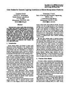
at Army-desired operational tempos.1 There are 3 steps to our method: 1) solve for the double derivative, 2) apply the optic flow algorithm of choice, and 3) isolate the true flow using a mask, as shown in Fig. 1. 1 2
Fig. 1
3
Flowchart of our proposed method, showing the 3 steps employed
Standard derivative calculations were used, incorporating both the x and y components. While several different filter operators were tried during the course of the project, we chose [1,–1] (or its transposed pair, for y). Numerous other standard filters (Gaussian, Laplacian, etc.) were tried and produced no significant increase in performance. Due to the continued focus on reducing the total number of computations required, a smaller filter operator was preferred: 𝜕𝜕𝜕𝜕 2
∇𝑓𝑓 = � 𝜕𝜕𝜕𝜕 +
𝜕𝜕𝜕𝜕 2
𝜕𝜕𝜕𝜕
−2
�
(1)
where 𝑓𝑓 = is the value of the pixel at the (x,y) position, and the second spatial derivative of f is the gradient of the image (∇f). Those areas of the image without any texture will result in no detected motion from the optic flow algorithms. To avoid biasing the state estimation and still allow for the possibility that there may not have been any ego motion, we created a mask to put over the resultant optic flow vector field. This mask is based on the informationpoor areas of the filtered image. Through experimentation, we found that masking all areas where the double derivative image pixel value was below 10 (on a scale of 0 to 255) removed the majority of the spurious data. A note on complexity. Let n = w x h be the number of pixels in each image frame. We assume the use of optic flow algorithms with input consisting of sequential pairs of frames in a time sequence. In the case of Lucas-Kanade, the time complexity of each iteration of optical flow is dominated by the computation of the Hessian, which is linear in n but quadratic in the number of warp parameters Approved for public release; distribution is unlimited.
4
m ( ≈ O(nm2)).22 In the case of iterative global methods such as Horn-Schunck, analysis of the computational cost has additional dependencies including whether the algorithm is allowed to converge. At its core, the Horn-Schunck algorithm is the Jacobi iterative method applied to the interior of the image23 and requires computation of first-order partial derivatives with a complexity at least linear in n.24 A highly optimized implementation may precompute certain pixelwise quantities prior to entering the iterative phase; even so, it has been demonstrated practically that Horn-Schunck requires, on average, substantially more computations per pixel than Lucas-Kanade.25 Our technique is a preprocessing step requiring a single convolution over each image to be taken as input to the chosen optic flow algorithm. The results of the derivative computation may be stored for later use at a cost no greater than that of the input image. Let k be the size of the convolution kernel (k = 2 in the method suggested above). We assert that the complexity of our method is linear in n and the subsequent masking operation requires constant time per pixel, resulting in an overall complexity O(nk + cn). We posit that this complexity is generally dwarfed by that of the downstream optical flow algorithm. The implementation of Lucas-Kanade26 employed for these experiments used 3 pyramids and 3 iterations. That of Horn-Schunck27 used an alpha of 1 and maximum iteration of 100. In both cases, the algorithms were received pre-tuned and were not altered. We are aware that this method is not robust to the “features” created by strong shadows. However, from our experience embedded with infantry units in realistic conditions and point of view (POV) video data gathered during those experiments, strong shadows remain relatively static. We are more concerned with dynamic changes such as the passage of clouds overhead, which will affect all shadows and lighting conditions equally. However, we have begun investigation into texture patterns, which may mitigate the shadow problem.
4.
Data
The images used in the following experiments were collected in a field at Ft. Benning, Georgia, during a live exercise28 using a GoPro Hero3 and in an office using a Logitech C920 Webcam. Stage lighting was used to create controllable and repeatable dynamic lighting conditions for the indoor space. The outdoor data collection occurred on a cloudless and extremely sunny day and the lighting is considered to be static. For ease of comparison, both data sets were collected with a static camera. To create the companion “dynamic motion” sets, the “static motion” sets were subsampled and only a portion of each successive frame was used. The location of this region Approved for public release; distribution is unlimited.
5
within the base image was altered by a known number of pixels, which became the ground truth for the optic flow estimations. To ensure the data were comparable, the static sets used an identically sized subsampled area from the original images – although in this case, the location of the window did not alter between frames. Each dataset is comprised of 100 sequential images, selections of which are shown below. There have been several datasets created to test visual state estimation under a variety of circumstances, most notably Kitti29 and Sintel.30 Both sets include a variety of lighting conditions; however, we did not find known illuminance values associated with the imagery. As this is preliminary work in which we hoped to explicitly measure the relationship between changes in illumination and the amount of noise added to an optic flow estimate, we chose to create our own dataset. In future iterations of this work, we plan to use established datasets to allow for rigorous comparison between methods.
5.
Experimental Scenarios
In the following scenarios, the phrase “algorithms” refers to both Horn-Schunck and Lucas-Kanade with both standard and prefiltered inputs.
5.1 Scenario 1: Static Camera, Static Lighting To ensure that any error was due to the input, rather than the algorithms, we first tested the performance of the optic flow methods using the statically lit dataset and a static camera location. With no motion and no sensory noise, an ideal output would show a cluster of dots around the (0,0) point.
5.2 Scenario 2: Static Camera, Dynamic Lighting In this case, we wished to measure how the algorithms responded to changes in illumination only. With a static camera and static scene, any resulting “motion” must be due to the illumination shift.
5.3 Scenario 3: Dynamic Camera, Static Lighting To determine how accurately each algorithm responded to actual motion, we tested them using a dynamic camera position and static lighting condition. In this scenario, any deviation from ground truth must be due to errors in state estimation of the algorithms themselves.
Approved for public release; distribution is unlimited.
6
5.4 Scenario 4: Dynamic Camera, Dynamic Lighting The final scenario investigates a mobile camera in dynamic lighting conditions. We feel this is the most similar to true field operation conditions and shows how accurate the algorithms’ state estimation is. In this case, deviation from ground truth is due to a combination of motion and lighting conditions.
6.
Results
The following graphs represent the results of processing the aforementioned lighting conditions with and without the prefiltering step. In each figure, the same camera path is shown in both static and dynamic lighting conditions. By showing how the algorithms respond to their expected input (statically lit images), as well as how they respond to the dynamic lighting, one can see which errors are due to the implementations of the algorithms and which are due to the input data format. Furthermore, we include the same implementation with and without the prefiltering step to show directly the difference it makes. The left column of each figure displays the actual plotted position of each state estimate as well as the true position, while the right column shows the Euclidean disparity between the estimate point and ground truth at each position in the run. Deviation is measured in pixels. Figure 2 shows the results of static (a,b) and dynamic (c,d) lighting on optic flow using data collection with a stationary camera to demonstrate the error, which is added to state estimation through variation in lighting alone. The camera is static; any perceived “motion” must be due to estimation error. As may be seen in the top row, all algorithms perform as expected, showing subpixel motion when presented with no motion and static lighting. However, in the bottom row, one may see the results of varied lighting conditions and that the filtered implementations are far more robust to its effects.
Approved for public release; distribution is unlimited.
7
Fig. 2 Measured responses for a static camera position and static picture with dynamic changes in lighting, where a) and b) show the position estimation and deviation from ground truth for scenario 1, and c) and d) show the results of scenario 2
Figure 3 shows the results of optic flow in both static (a,b) and dynamic (c,d) lighting conditions as captured by a dynamic camera. In this case, motion may be due to either an actual change or lighting, although as may be seen by comparing the top (static lighting) and bottom (dynamic lighting) rows, all algorithms perform well in static lighting, while the prefiltered versions are far more robust in the dynamic conditions.
Approved for public release; distribution is unlimited.
8
Fig. 3 Measured responses for a dynamic camera position and static picture with dynamic changes in lighting, where a) and b) show the position estimation and deviation from ground truth for scenario 3, and c) and d) show the results of scenario 4
As anticipated, the standard-input optic flow algorithms produce nearly perfect results in static lighting conditions, with a mean error of 1.6 pixels for both algorithms and a standard deviation of 0.77 and 0.79 for Horn-Schunck and LucasKanade, respectively. The prefiltered version results overshot the mark slightly, with mean errors of 4.8 and 5.9 pixels and standard deviations of 2.8 and 3.5 pixels for Horn-Schunck and Lucas-Kanade, respectively. However, in dynamic lighting conditions, the prefiltered results remain very close to the ground truth and do not deviate significantly over time. In this case, they averaged 1.8 and 4.1 pixels of error with standard deviations of 0.7 and 2.2 pixels for Horn-Schunck and Lucas-Kanade, respectively. Conversely, the standard input algorithms are not reliable under such conditions, with mean errors of 10.9 and 31.45 pixels, with standard deviations of 5.1 and 33.7 pixels for Horn-Schunck and Lucas-Kanade, respectively. The prefiltered optic flow does better in dynamic lighting than it does in static, and we are currently investigating how this can be generally applied. Approved for public release; distribution is unlimited.
9
To begin testing the boundaries of this method, we created the experiment presented in Fig. 4 by comparing a reference image at a known illumination to a series of other images of the same object, captured at a variety of known illumination levels. The algorithms used here are identical to those used earlier in the report. For context, a change of 100 lux is within the deviation allowed within a well-lit office. Realistically, changes in illumination are often far more radical. A cloud passing in front of the sun can easily case variations on the order of 5,000 lux. While the degree of variation in illuminance from frame to frame is dependent on the frame rate of the camera and the conditions the system is operating in, our method’s robustness to changes of over 600 lux per transition and our planned frame rate of 30 fps gives us confidence that even and indoor/outdoor transition of 10,000 lux would be manageable.
Fig. 4
7.
Filtered and unfiltered optic flow’s responses to extreme variations in illuminance
Conclusion
The primary assumption of traditional optic flow is that illumination remains constant, and under such conditions, it performs admirably. However, the real world is a dynamic and irregular place and any system that intends to operate within it must be robust to constantly changing conditions. As shown in Figs. 2 through 4, simply by changing the input from a standard image to the double derivative of that image, we are able to produce a significant increase in position estimation accuracy under dynamic lighting conditions. The next big push in robotics is for small, autonomous systems to quickly navigate complex environments, specifically, below the canopy in forests.1 We have found that prefiltering is a useful tool for real-world navigation and particularly for size, weight, and power (SWaP)-constrained systems that cannot Approved for public release; distribution is unlimited.
10
carry more than a single camera. It is computationally reasonable, as creating an image double derivate is substantially less expensive than the host optical flow algorithm and does not require any sort of a priori information. Our approach is robust to significant variations in lighting, while also being very easily implemented and added to existing system. Despite the information lost by taking the derivative of the image prior to optic flow calculations and the subsequent masking of the dead zones, we find that sufficient, relevant information persists for this method, producing useful results.
8.
Future Work
There is still a great deal of work to be done in order to make optic flow robust to the vagaries of outdoor operation. We plan to investigate how best to identify and eliminate features due to strong shadows rather than actual environmental features. Despite the strong edges and image variations caused by shadows, the textures of the objects within the scene remain the same. We have considered a method that compares the patterns and significant deviations. Another typical source of error are dynamic backgrounds, such as windblown trees and grass. Such objects have fixed locations, but nonetheless add a great deal of noise to the vector field and disrupt the flow patterns usually used to determine ego motion and the presence of outside agents. Furthermore, when resident on a vehicle, there are likely to be ego-motion errors, such as vehicle drift and vibration, which will need to be accounted for. We look forward to combining all of these problems in future investigations into dynamic environments with highly constrained systems.
Approved for public release; distribution is unlimited.
11
9.
References
1.
Micire M. Fast Lightweight Autonomy (FLA). Defense Sciences Office, DARPA; 22 Dec. 2014 [accessed 10 Feb. 2015] http://www.darpa.mil/program/fast-lightweight-autonomy.
2.
Bohren J, Foote T, Keller J, Kushleyev A, Lee D, Stewart A, Vernaza P, Derenick J, Spletzer J, Satterfield B. Little Ben: The Ben Franklin racing team’s entry in the 2007 DARPA urban challenge. J. Field Robotics. 2008;25:598–614. doi: 10.1002/rob.20260.
3.
Lucas B, Kanade T. An iterative image registration technique with an application to stereo vision. IJCAI. 1981;81.
4.
Krapp H, Holger, Hengstenberg R. Estimation of self-motion by optic flow processing in single visual interneurons. Nature. 1996;384(6608):463–466.
5.
Horn B, Schunck B. Determining optical flow. In: 1981 Technical Symposium East. International Society for Optics and Photonics, p. 319–311.
6.
Schlyter P. Radiometry and Photometry in Astronomy: How bright are natural light sources; 18 Mar 2009 [accessed 5 Feb 2015] http://stjarnhimlen.se/comp/ radfaq.html.
7.
Dederscheck D, Muller T, Mester R. Illumination invariance for driving scene optical flow using comparagram preselection. IEEE 2012. Proceedings of Intelligent Vehicles Symposium (IV); 2012 Jun 3–7; Madrid (Spain): IEEE.
8.
Zhang L, Tatsunari S, Hidetoshi M. Detection of motion fields under spatiotemporal non-uniform illumination. Image Vision Comp. 1999;17(3):309– 320.
9.
Mileva Y, Yana Invariance with optic flow [dissertation]. [Saarbrücken (Germany)]: Saarland University; 2007.
10. Mileva Y, Bruhn A, Weickert J. Illumination-robust variational optical flow with photometric invariants. Pattern Rec. 2007;4713:152–162. 11. Van de Weijer J, Gevers T, Smeulders A. Robust photometric invariant features from the color tensor., IEEE Trans on Image Processing. 2006;15(1):118–127. 12. Schuchert T, Aach T, Scharr H. Range flow in varying illumination: Algorithms and comparisons., IEEE Trans on Pattern Analysis and Machine Intelligence. 2010;32(9):1646–1658. Approved for public release; distribution is unlimited.
12
13. Kendoul F, Fantoni I, Nonami K. Optic flow-based vision system for autonomous 3D localization and control of small aerial vehicles. Robotics and Autonomous Systems. 2009;57(6):591–602. 14. Haussecker H, Fleet D. Computing optical flow with physical models of brightness variation. IEEE Trans on Pattern Analysis and Machine Intelligence. 2001;23(6):661–673. 15. Zimmer H, Bruhn A, Weickert J, Valgaerts L, Salgado A, Rosenhahn B, Seidel H.. Energy minimization methods in computer vision and pattern recognition. Berlin (Germany): Springer Berlin Heidelberg; 2009 January. Chapter 16, Complementary optic flow; p. 207–220. 16. Kearney J, Thompson W, Boley D. Optical flow estimation: An error analysis of gradient-based methods with local optimization., IEEE Trans on Pattern Analysis and Machine Intelligence. 1987;2:229–244. 17. Enkelmann W. Obstacle detection by evaluation of optical flow fields from image sequences. Image and Vision Comp. 1991;9(3):160–168. 18. Christmas W. Filtering requirements for gradient-based optical flow measurement. IEEE Trans on Image Processing. 2000;9(10):1817–1820. 19. Lempitsky V, Roth S, Rother C. Fusionflow: Discrete-continuous optimization for optical flow estimation. In: CVPR 2008. Proceedings of the IEEE Conference on Computer Vision and Pattern Recognition; 2008 Jun 23–28; Anchorage (AK): IEEE; June p. 1–8. 20. Sellent A, Eisemann M, Goldlücke B, Pock T, Cremers D, Magnor M. Variational optical flow from alternate exposure images. In: VMV 2009. Proceedings of the Vision, Modeling and Visualization Conference; 2009 Nov; Braunschweig (Germany); p. 135–144. 21. Sharmin N, Brad R. Optimal filter estimation doe Lucas-Kanade optical flow. Sensors. 2012;12(9):12694–12709. 22. Baker S, Matthews I. Lucas-Kanade 20 years on: a unifying framework. Intl J Comp. 2004;56(3):221–255. 23. Kameda Y, Imiya A, Ohnishi N. Combinatorial image analysis. Berlin (Germany): Springer Berlin Heidelberg; 2008. Chapter 24, A convergence proof for the Horn-Schunck optical-flow computation scheme using neighborhood decomposition; p. 262–273.
Approved for public release; distribution is unlimited.
13
24. Anderson M, Iandola F, Keutzer K. Quantifying the energy efficiency of object recognition and optical flow. Berkley (CA): Dept. of Electrical Engineering and Computer Sciences California Univ Berkeley; 2014 Mar 28. Report No.: UCB/EECS-2014-22. 25. Bruhn A, Weickwert J, Schorr C. Lucas/Kanade meets Horn/Schunch: Combining local and global optic flow methods. Intl J Comp Vision. 2005;61(3):211–231. 26. Bilgic B. Iterative pyramidal LK optical flow. Matlab 7.6 (R2008a). 27 Feb. 2009. MathWorks File Exchange [accessed 26 Jan 2015] http://www.mathworks.com/matlabcentral/fileexchange/23142-iterativepyramidal-lk-optical-flow. 27. Kharbat M. Horn-Schunck optical flow method. Matlab 7.4 (R2007a). 22 Jan. 2009. MathWorks File Exchange [accessed 26 June 2014] http://www.mathworks.com/matlabcentral/fileexchange/22756-hornschunck-optical-flow-method. 28. Brayboy J. Research lab to test insect-inspired robotic platform in Army exercise. ARL News. Army Research Laboratory (US), 7 Nov 2014 [accessed 6 Feb. 2015] http://www.arl.army.mil/www/?article=2549. 29. Geiger A, Lenz P, Urtasun R. Are we ready for autonomous driving? The kitti vision benchmark suite. In: CVPR 2012. Proceeding of the IEEE Conference on Computer Vision and Pattern Recognition; 2012 Jun 16–21; Providence (RI); p 3354–3361. 30. Butler D, Wulff J, Stanley G, Black M. A naturalistic open source movie for optical flow evaluation. In: ECCV 2012. Proceeding from the European Conference on Computer Vision; 2012 Oct 7–13; Florence (Italy); Springer Berlin Heidelberg; p. 611–625.
Approved for public release; distribution is unlimited.
14
List of Symbols, Abbreviations, and Acronyms DARPA
Defense Advanced Research Projects Agency
EMD
Elementary Motion Detector
EO
electro-optic
HSV
hue-saturation-value
IM
intensity modulated
POV
point of view
RGB
red-green-blue
SWaP
size, weight, and power
UAS
unmanned aerial system
UAV
unmanned aerial vehicle
Approved for public release; distribution is unlimited.
15
1 DEFENSE TECHNICAL (PDF) INFORMATION CTR DTIC OCA 2 DIRECTOR (PDF) US ARMY RESEARCH LAB RDRL CIO LL IMAL HRA MAIL & RECORDS MGMT 1 GOVT PRINTG OFC (PDF) A MALHOTRA 6 DIRECTOR (PDF) US ARMY RESEARCH LAB RDRL SER A MATHIS W NOTHWANG D DONAVANIK J CONROY J SHAMWELL R ROBINSON
Approved for public release; distribution is unlimited.
16