MAP inference in Large Factor Graphs with Reinforcement Learning ...

MAP inference in Large Factor Graphs with Reinforcement Learning Khashayar Rohanimanesh, Michael Wick, Sameer Singh, and Andrew McCallum CMPSCI Technical Report UM-CS-2008-040

December 7, 2008 Department of Computer Science University of Massachusetts 140 Governors Drive Amherst, Massachusetts 01003

Abstract Large, relational factor graphs with structure defined by first-order logic or other languages give rise to notoriously difficult inference problems. Because unrolling the structure necessary to represent distributions over all hypotheses has exponential blow-up, solutions are often derived from MCMC. However, because of limitations in the design and parameterization of the jump function, these sampling-based methods suffer from local minima—the system must transition through lower-scoring configurations before arriving at a better MAP solution. This paper presents a new method of explicitly selecting fruitful downward jumps by leveraging reinforcement learning (RL) to model delayed reward with a log-linear function approximation of residual future score improvement. Our method provides dramatic empirical success, producing new state-of-the-art results on a complex joint model of ontology alignment, with a 48% reduction in error over state-of-the-art in that domain.

1

Introduction

We focus on structured output prediction problems in large factor graphs where the hidden variables are not independent, but have a complex internal structure (label sequence, trees, partitions, etc) as it is commonly the case in many Natural Language Processing tasks (parsing), Information Retrieval (coreference resolution), and Database Systems (ontology alignment). Unfortunately, most of general techniques for performing learning and inference in such complex models are computationally expensive; therefore, many of the previous applications have been restricted to label sequence prediction in simpler graphical structures (for example making linear chain assumption as in likelihood based models such as hidden Markov models (HMMs) [19], maximum entropy Markov models (MEMMs) [16], linear-chain conditional random fields (CRFs) [13], max-margin Markov networks [22], support vector machines for structured outputs [26], case-factordiagams [14], sequential Gaussian process models [1], and search based structure prediction [11, 10]). Most of these models perform gradient descent on the log-likelihood or marginals which involve computing expectations of features given the model’s sufficient statistics. Alternatively, margin-based methods (M-cubed [22]) requires solving a quadratic program (QP) to satisfy a set of constraints that demands the ground-truth configurations outweigh the rest. Although certain modeling assumptions (e.g., linear-chain graphs) allows the computational complexity to be reduced, training such models remains expensive. Parameter estimation is therefore difficult in both approaches because of the reliance on expensive inference procedures: likelihood-based models require marginals for computing feature expectations, and margin-based models require both computing marginals, and top-n configurations for constraints in the quadratic program. The perceptron[4] remedies the need for computing expensive marginals; however, it still depends on a decoding step that requires solving the MAP problem in such models [18]. To further illustrate this, consider a conditional random field (CRF) modeling a complex structured prediction problem in terms of a conditional probability distribution P (Y |X, θ) where θ is a parameter vector. The decoding problem (or MAP inference) is defined as: y ∗ = arg max P (y | x, θ) y∈Y

2

It is known that decoding is intractable for large arbitrary graphs. Therefore, even if we use the perceptron to avoid computing marginals, learning is still costly because we must perform a decoding step in every single update. There have been two different approaches that attempt to alleviate this problem by reducing the requirement for computing the decoding step (computing the arg max). The first approach (known as LASO[11] and SEARN [10]) formulates the problem as search optimization where a search cost function is learned to score partial configurations that potentially lead to a goal state. A perceptron style update is then used to adjust the parameter vector whenever the model makes an incorrect prediction about a partial configuration. In contrast, the second approach (SampleRank [6]) learns to rank complete configurations according to their relative merits based on the ground truth information. Whenever the model prediction about the rank of a configuration pair is incorrect, a perceptron style update is performed to adjust the model parameters. At test time, the system performs a simulated annealining procedure from a random initialization point in order to arrive at the MAP configuration through a series of transitions. Although these approaches reduce the learning/inference complexity in large models, they host a set of new challenges: • LASO/SEARN: This approach relies on a monotonicity assumption: a partial configuration is classified as y-good if it can lead to an output configuration y. The 0/1-loss nature of this requirement essentially ignores many partial configurations that are only marginally imperfect but potentially provide useful information. This property is also somewhat undesirable in cases where we may want to start the search in a full (imperfect) configuration predicted by another system. Moreover, if the search cost is not an admissible heuristic, it turns into a heuristic search which may not arrive at the optimal solution. • SampleRank: (1) SampleRank’s performance is sensitive to the quality of the learned rank function. Due to a combinatorial number of ranking constraints, a log-linear representation of the rank function may not be able to satisfy all the constraints. Thus, at test time it is possible that the model could get stuck in a local minima while hill climbing over an imperfect ranking function; (2) SampleRank employs a proposer for generating a set of candidate configurations that can be transitioned to from the current state. Therefore, there is a trade-off between the computational cost of scoring the candidates and the ergodicity of the Markov chain induced by the proposer: when more complex moves are proposed, more factors must be computed for prediction. SampleRank encourages simpler proposers for computational gains. Because of this requirement, it is possible that SampleRank may not monotonically climb the ranking function with a single move, and may need to perform several moves in a sequence—possibly lowering the performance in order to get in a better configuration over the long run. This is further illustrated in Figure 1: the top path shows a sequence of moves from some configuration s1 that would possibly lead to the goal configuration (marked by G). Now consider a simple proposer that would propose either a split (split partition X1 which results in configuration s2 ) or merge (merge partitions X1 and X2 which results in configuration s4 ). Note that if the system accepts the merge, the F 1 score may temporarily go up, however in the long run. the split choice is a more optimal move even though F 1 score temporarily suffers in state s2 . In fact, configuration s2 is a better state for arriving at the goal than s4 . To understand why s4 is not the best state to transition to in the long run, note that in future moves, 3

we must split the partition X0 to reach the goal; yet, the probability of achieving the desired split in a single move is 2|X1 0 | .

S2

S3 Y4

Y4

...

...

X4

Y1 Split(X1)

Y3

...

... ..

.. .

4

6

Y5

X1

... X X

X5 Merge(X4,X2)

Y3

.. .

X2

Y12

Y3

Y23

X

Y35 Y6

Y2

G Y7

X2

Y78

Merg(X1,X2)

X3

Y23

Y8

Y2

S1

Y79

Y0

.. .Y

...

Y89

3

X0

Y9 Y03 X3

t

S4

t+1

t+2

t+n .. .

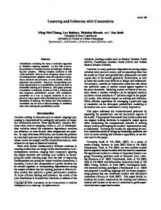
Figure 1: . This can be illustrated further in a concise example, demonstrating how an MCMC method may have difficulties transitioning through certain areas of the feasible region during inference, even with the assistance of a truth signal. Imagine a situation where there are two ground truth clusters: A and B with n instance of A and m instances of B. Figure 2 shows a seemingly simple case where m = n = 5. Beginning with each instance in the same cluster, we would like to find the MAP configuration using an MCMC algorithm that can modify a single variable at a time. However, if we compute the pairwise F1 for the states along the optimal sequence to the goal, we discover that a downhill move must be made immediately and that many states on the path have lower score than the starting state. Figure 3 contains the pairwise F1 scores for the states along the optimal sequence beginning with a single cluster and ending with the MAP configuration (for the case where m = n = 20). We can see that four downhill transitions must be executed

4

P =.44 R =1.0

P =.34 R =.80

P =.48 R =.70

P =1.0 R =1.0

F1=.61

F1=.48

F1=.57

F1=1.0

Figure 2: The optimal sequence of moves required to split two clusters using a proposal distribution that can modify a single variable at a time. Note that the moves along the optimal sequence to the MAP configuration have F1 (pairwise) scores lower than the initial configuration, making it difficult for MCMC to sample them. while traversing the optimal path; in high dimensional spaces, there may be a large number of downhill (and uphill) moves to consider from each state, particularly in problems where there are more than just two clusters. Exploring these moves randomly is likely to result in slow progress through the state space and may even require an exponential number of samples to arrive in the MAP configuration. One approach to cope with this difficulty is to craft more sophisticated proposal distributions that allow MCMC to make larger modifications to the configuration space in a single transition. However, this does not fix the problem in general because it blows up the transition space of the proposal distribution. For example, in a split-merge proposer, the probability of optimally splitting 1 a cluster is 2k−1 where k is the size of the cluster. Another difficulty encountered by samplers is that the ground truth signal can be so poorly behaved for structured prediciton problems and annealing may not be adequate to overcome local optima. While truth signals are known to behave poorly in terms of the immediate costs (and benefits) incurred by a proposal distribution, all evaluation metrics share one important trait: the ground truth configuration has a globally optimal score. Intuitively, truth signals are well-behaved around the goal, leading us to believe these functions exhibit good behavior in the long run. Taking into account the above discussion with an emphasis on the delayed feedback nature of the problem immediately inspires us to employ reinforcement learning (RL) for MAP inference. RL is a framework for solving the sequential decision making problem with delayed reward. There has been an extensive study of this problem in many areas of machine learning, planing, robotics, etc. To the best of our knowledge our approach is the first attempt to apply reinforcement learning to MAP inference in large factor graphs. In addition to the ability of RL to cope with the delayed 5

0.66 0.65 0.64 0.63 0.62 0.61 0.6 0.59 0

1

2

3

4

5

6

7

8

9

20

Figure 3: A plot of the pairwise F1 scores of each state along the optimal transition sequence to the MAP configuration for the case where there are twenty objects of both types. Notice that several consecutive downhill transitions must be executed to reach the MAP state. feedback, we find this framework suitable for for several reasons: (1) to achieve generalization RL is integrated with function approximation schemes, in particular linear function approximation has been extensively studied [21]. (2) Value functions in RL smooth out the noise in predictions by backing up values from neighboring states. This property of value function should mitigate the impact of a noisy prediction (a problem SampleRank does not address). In other words, even if a SampleRank decision would have resulted in a poor configuration due to the noise in the learned rank function, the RL would be less susceptible to such imperfections since the value function (informally speaking) averages across the predictions, given a current configuration. Each state in the system represent a complete assignment to the hidden variables Y . From a clustering perspective, if X is the set of observed inputs (e.g., mentions in a coreference resolution problem), there will be Bell(|X|) possible assignment which yields a combinatorially large state space. To cope with such a complexity we employ linear function approximation techniques to generalize across the state space. For any given state, the set of actions in general could be again defined as any assignment to the hidden variables. Note that there exists a tight connection between the notion of an action and a state. In order to cope with complexity in the action space, we introduce a proposer that constrains the space by limiting the number of possible actions from each state (and possibly more useful when domain-specific knowledge is injected in the proposer). . For example, in a clustering application, we could use a uniform proposer [12] that would only allow the system to split a randomly selected cluster, or to merge a random pair of clusters. In general there exist a trade off between the complexity of the proser and learning performance: the more complex the proposer, the larger the set of actions to be explored during learning. More 6

complex actions could help transition across the configuration space in fewer steps, however they may slow the learning process because more exploration is needed. The reward function can be defined as the residual performance improvement when the systems transitions from current state to the next state. In our approach we use a performance measure based on the ground truth labels (for example F1 score using BCUBED metric). Note that at test time we do not have access to the ground truth labels, thus we do not have access to a reward signal. To address this issue, we propose two different approaches: (1) in the first approach we first learn an approximation of the reward function at training time, and then use that at test time to compute an approximation of the optimal value function value function and the optimal policy; (2) in the second approach we directly learn a generalizable value function a training time using a performance measure based on ground truth labels as the reward signal. At test time, we perform a policy search by hill climbing the approximate value function computed in the test domain. We also present our preliminary results in a coreference resolution problem. As the number of states can get pretty large, linear function approximation techniques are employed to generalize across the state space. Although there are no convergence proofs for pure value-based RL methods with function approximation, in practice it has been successful in a number of problems [5, 32, 23]. The log-linear nature of CRFs allows us to readily apply the related algorithms to CRFs. To the best of our knowledge, our approach is the first attempt to apply reinforcement learning to MAP inference in factor graphs. Our approach in spirit is similar to [30] where they propose a reinforcement learning framework for solving combinatorial optimization problems. Similar to this approach, we also rely on generalization techniques in RL in order to directly approximate a policy over the unseen test domain. However, our formulation provides a framework that explicitly targets the MAP problem in large factor graphs and takes advantage of the log-linear representation of such models in order to employ a well studied class of generalization techniques in RL known as linear function approximation. Learning a generalizable function approximator has been also used in standard search algorithms for efficiently guiding the search by learning evaluation functions from experience [3]. The rest of this document is organized as follows: in § 2 we briefly overview background material. In § 3 we describe the details of our algorithm and discuss a number of ideas for coping with the combinatorial complexity in both state and action spaces. In § 4.4 we present our preliminary empirical results, and finally in § 5 we conclude and lay out a number of ideas for future work.

2

Background

This section serves to provide background information about conditional random fields (a discriminative factor graph), SampleRank (an approach to learning the parameters of the graph), and methodology of reinforcement learning.

7

2.1

CRF

A conditional random field (CRF) is a discriminative factor graph that gives a conditional probability distribution over an assignment to some hidden variables Y=y given a set of observed variables X=x. That is, a CRF can be written in the form: P (Y = y|X = x) =

1 Y ψ(X, y i ) ZX i y ∈M

where ZX is an input-dependent normalizing constant ensuring that the distribution sums to one. The structure of the CRF is determined by the factors ψ(X, y i ), that decompose the model into sets of Y variables y i ∈ M where M ⊆ P(Y ). A factor is a function that maps an arbitrary number of hidden (y i ) and observed variables (X) to a real-value. Often the factors are designed in such a way to make exact learning and inference tractable (for example, linear-chains), but in practice, we would like arbitrary structures; for example, clustering problems contain graphs with loopy and highly connected structures. Typically CRF factors are log-linear combinations of features φ(X, y i ) and parameters θ = {θj }: ψ(X, y i ) = exp(φ · θ). Learning is typically performed with some form of gradient descent, which requires computing the derivative of the log-likelihood with respect to each parameter: X X X ∂l logL(Y ; X, θ) = λk gk (X, y i ) − θk gk (X, y i ) ∂θk i i Y

y ∈M

y ∈M

however, the above gradient involves model expectation over features, requiring a summation over all configurations Y = y. One method for overcoming this difficulty is a piece-wise approximation [17] to the model. This is done by sampling examples of the yi hidden variables from a labeled training set for each factor independently. Since factors are log-linear, this training method reduces to learning a logistic regression classifier. The second method, called SampleRank [6], does not require partitioning the model into pieces and actually trains it in a global fashion. The algorithm assumes MAP inference is performed with Markov Chain Monte-Carlo and then updates parameters with approximate gradients at each MCMC step. More specifically, each step of MCMC induces a neighbor configuration pair by modifying a configuration y to produce y 0 . If the number of y variables modified is a constant, then the difference between y 0 and y is small and computing their gradient is efficient (specifically, this can be done with a linear number computations) for more details refer to [6]. Then the update rule can be applied as follows: ( −α φy,y0 if F(y) > F(y 0 ) ∧ θ · φy,y0 > 0 θ=θ+ α φy,y0 if F(y) < F(y 0 ) ∧ θ · φy,y0 ≤ 0

8

where θ is the current parameters, φy,y0 is the difference between the two state representations, F(y) is a ground truth metric used for training, and η(y, y 0 ) is a Bernoulli acceptance disribution, that determines whether or not to accept the next state y 0 . Maximum a posteriori (MAP) inference is the problem of finding the configuration y that maximizes the conditional probability P (Y ; X, θ). Since finding the optimal clustering in general CRFs requires exploring all possible configurations, we must resort to approximations. The greedy agglomerative search procedure works by initializing the configuration to all singletons (clusters with just one mention) and iteratively merges the clusters with the highest affinity, until a threshold τ is reached, at which point the algorithm terminates. The MCMC approach relies on a proposal distribution q that generalizes the agglomerative nature of the greedy process above. The proposal distribution stochastically proposes modifications to the configuration that could be either a random merge or split. This is in contrast to greedy agglomerative which can only propose greedy merges. Search also involves Bernoulli acceptance distribution η that probabilistically determines whether or not to accept the move proposed by q. 0 )q(y 0 →y) Setting η = p(y p(y)q(y→y 0 ) reduces our search procedure to the Metropolis-Hastings algorithm.

2.2

Reinforcement Learning

Reinforcement Learning (RL) refers to a class of problems in which an agent interacts with the environment and the objective is to learn a course of actions that optimizes a long term measure of a delayed reward signal. The most popular realization of RL has been in the context of Markov Decision Processes (MDPs). In this section we briefly overview MDPs, and introduce basic reinforcement learning concepts and algorithms that will be used throughout the rest of document. Most of the discussion here is based on [21]. 2.2.1

Markov Decision Processes

A finite Markov Decision Process (MDP) is defined by a tuple M = hS, A, R, Pi, where: • S is a finite set of states • A is a finite set of actions • R : S × A × S → R is the reward function, i.e. R(s, a, s0 ) is the expected reward received when action a is taken in state s and transitioning into state s0 . • P : S × A × S → [0, 1] is the transition probability function, i.e. P a (s, s0 ) is the probability of reaching state s0 if action a is taken in state s. A stochastic policy π is defined as π : S × A → [0, 1] where π(s, a) is the probability of choosing action a as the next action when in state s. In some cases, the policy may be deterministic, in which case π(s, a) is 1 for one of the actions, and 0 for the rest. Following a policy on an MDP

9

results in an expected discounted reward Rt accumulated over the run, where Rt =

T X

γ k rt+k+1 .

k=0

Hence an optimal policy π ∗ is defined as the policy which maximizes the expected discounted reward accumulated on the MDP. 2.2.2

Optimal Policy

Typically, optimal policy cannot be found directly. Instead, a value function is associated with the policy π, defined as Qπ : S × A → R where Qπ (s, a) defines the expected long term discounted reward starting at the state s, taking action a, and following the policy π. Similarly an optimal value function Q∗ is defined as Q∗ (s, a) = maxπ Qπ (s, a). The optimal value function be calculated using the Bellman equations[2],   X ∗ a 0 0 ∗ 0 0 Q (s, a) = P (s, s ) R(s, a, s ) + γ max Q (s , a ) 0 a

s0

2.2.3

TD-Learning

In many domains, however, we either do not have access to the complete model (reward function, and transition probabilities) or even if the model is available, in large domains the computational complexity of solving Bellman equations exactly becomes intractable (e.g., Back-gammon game [24]). Methods of temporal difference learning (TD) [20] were introduced that enables the agent to learn from pure experience in the absence of the model. TD methods are essentially a combination of Monte Carlo and dynamic programming (DP) techniques for solving the RL problem. In particular, Q-Learning[27] describes a TD method in the context of MDPs for learning the state-action value function (i.e., the Q values). While the agent interacts with the environment by following the current policy, the Q-values are updated as: h i Q(st , at ) ← Q(st , at ) + α rt+1 + γ max Q(st+1 , a) − Q(st , at ) a

This algorithm was further improved to Q(λ) by including the concept of eligibility traces. Eligibility traces are values stored with each state and action that represent the recency and the frequency of visits to that state and action. They are used as an indication of the amount of credit the state-action pair should receive when backing up rewards, the higher the eligibility trace, higher the reward it receives[20]. Q(λ) changes the Q-Learning update to include eligibility traces et (s, a) as follows, h i Q(st , at ) ← Q(st , at ) + α et (s, a) rt+1 + γ max Q(st+1 , a) − Q(st , at ) a

This algorithm provides a simple yet efficient method to learn the Q-values. It has strong theoretical convergence guarantees, and in practice finds the optimal policy fairly quickly.

10

2.2.4

Functional Approximation

This algorithm as explained is limited to very small domains since it involves storing a value for each state-action pair. This problem is averted by introducing function approximation to reinforcement learning[25]. The state-action pair hs, ai is now represented by a feature vector φ(s, a), where each feature φk ∈ φ(s, a) may be binary or real valued. The Q value is represented using a functional approximator that uses vector of parameters θ, i.e. Q(s, a) = Λθ (φ(s, a)) For this paper, we restict ourselves to linear function approximation, i.e. X θk φ k Q(s, a) = Λθ (φ(s, a)) = φk ∈φ(s,a)

Instead of updating the Q values directly as in the table lookup case, the updates are made to the parameters θ using a perceptron style update. δ ← rt+1 − Q(st , at ) + γ max Q(st+1 , a) a → − → − θ ← θ + αδ Eligibility traces are also handled differently. When used with function approximation, an eligibility trace cannot be stored for each state. Instead, an eligibility trace is stored for every feature, and these traces are accumulated for each feature individually. Since most of the features being used are not binary, a form of eligibility traces that applies to arbitrary feature vectors is used (Section 8.2,8.3 in [21]). The updates to the eligibility traces are reset during the exploratory stage, and are otherwise, → − − e ← γλ→ e + φ(s, a) → − → − − θ ← θ + α→ eδ

3

Proposed Approach

Conventionally, reinforcement learning has been used in control tasks, i.e. to control agents that are trying to maximize long-term rewards; such a setting requires a very different state and action space than in the factor graph domain. The problem of learning in factor graphs does not fit directly into the traditional reinforcement learning framework. However, by formulating the state, action and reward function carefully, we can solve MAP inference in a reinforcement learning framework and build on the wealth of techniques and practical experience available in this area of machine learning. The problem of learning in factor graphs can be framed as a combinatorial optimization problem since we have the scoring function over every possible configuration, and we want to find the 11

configuration with the highest score. Reinforcement Learning has been applied to combinatorial optimization problems[31, 32, 9]. Even though the problem appears to be similar to these, a number of concerns need to be addressed before reinforcement learning methods can be used. In the following section, the problem of MAP inference in factor graphs is described as a reinforcement learning task. When formulating the MAP inference problem in factor graphs as a Markov Decision Process (MDP), each state represents a possible assignment to the variables hidden Y (for example in coreference resolution task a particular clustering of the mentions). The actions generally can be thought of as any changes to the assignment of the Y variables, however as we mentioned in Section 1 we need to carefully constrain the action space in order to cope with the complexity of learning. A reward function can be defined over these states and actions that shall ensure the states (e.g., clusterings in a coreference domain) with the highest score is reached when the optimal policy is followed. Formally, we can define an MDP M = hS, A, R, Pi with set of states S, set of actions A, reward function R, and transition probability function P formulating the MAP inference problem as follows:

3.1

States

Recall that our objective is to find the MAP configuration by optimizing a sequence of moves in the configuration space when the system is initialized in some arbitrary configuration. This immediately suggests that the state space in the RL formulation should encapsulate the entire feasible region. In terms of the CRF (or more generally, a factor graph) representation of the problem, a state is any assignment to the variables Y . Equivalently, when we view the problem as clustering (for example in coreference resolution problem), each possible clustering corresponds to a single state in the RL formulation. As explained in Section 1 in this particular view the state space has Bell(|X|) complexity. To cope with such a combinatorial state space we will have to exploit efficient generalization techniques in RL as we will describe in the following sections.

3.2

Actions

Given a state s (e.g., an assignment of Y variables), an action can be defined as a constrained set of modifications to a subset of the variables in state s. As discussed in Section 1, in general, any possible changes to the variables can be interpreted as an action, however this renders a combinatorial set of actions which is undesirable. One way to constrain the action space to a manageable size is to use a proposer, or a behavior policy from which actions are sampled. For example when the problem is framed as clustering, a uniform split/merge proposer could be used to generate sample actions in every state. This choice of a proposer limits the number of ways we can modify the current state since it only allows for splitting a randomly selected cluster, or merging a random pair of clusters. Note that in general we can exploit the domain knowledge to design more efficient proposers. From a different perspective, a proposer defines the set of reachable states by describ-

12

ing the distribution over next states s0 given a state s. The proposer, when regarded in context of the action space of an MDP, can be viewed in two ways. First, each possible next state s0 can be considered the result of an action a, leading to a large number of deterministic actions. Second, it can also be regarded as a single highly stochastic action, whose next state s0 is a sample from the distribution given by the proposer. Both of these views are equivalent; we use the former view for notation simplicity.

3.3

Reward Function

The reward function should be designed in such a way that the policy optimizing it in the long run takes us to the goal state (i.e., MAP configuration, or in the context of coreference resolution, the clustering with the highest score based on the ground truth labels). In general RL gives us total freedom on how to specify the reward function. In our approach we formulate the reward function in connection with the goal state (i.e., MAP configuration). As in many reinforcement learning implementations, the shortest path to the goal is obtained by giving a non-negative reward at the goal state, and giving a reward of −1 in non-goal states (also known as minimum-distance-togoal reward function). This reward function requires extensive exploration before the goal state is reached, which will not scale well to large combinatorial domains. Since the space is combinatorial, rewards must be shaped in such a way that at every state it facilitates efficient learning. Now, let F be some performance metric (for example, for information extraction tasks, it could be F 1 score based on the ground truth labels). A number of possible reward functions are described below: • We can define an absolute distance between from the current state to the goal state according to the performance metric: R(s) = F(s) − F(sG ) note that when F = F1, we have R(s) = F1(s) − 1. This reward function specifies the Euclidean distance between the current state and the goal state based on the F distance metric. • Alternatively, we can specify a reward function based on the residual improvement based on the performance metric F when system transitions from some state s to s0 : R(s, s0 ) = F(s0 ) − F(s) note that when F = F1, we have R(s, s0 ) = F1(s0 ) − F1(s). This reward function resembles the geodesic distance between the current state and the goal state based on the F distance metric. One important point to note is that we only have access to the ground truth labels at training time. One would wonder how we would apply RL at test time, and in the absence of the ground truth labels (which implies the reward function is not immediately available). We will describe two different approaches to cope with this problem in Section 3.5.

3.4

Transition Probability Function

Recall that the actions in our system are samples generated from a proposer B, and that each action uniquely identifies a next state in the system. The function that returns this next state determin13

istically is called simulate(s,a). Thus, given the state s and the action a, the next state s0 has the following probability:  0 s0 6= simulate(s, a) a 0 P (s, s ) = 1 s0 = simulate(s, a) The probability that the next state is s0 given that the current state is s hence corresponds to X P(s, s0 ) = P (B(s) = a) P a (s, s0 ) a

3.5

Algorithms

Once the state, action space and the reward function have been defined, we can now employ various RL learning algorithms in order to learn the optimal policy (or near optimal) for arriving in MAP configuration when the system is initiated in some arbitrary configuration. Before specifying the details of the algorithms, we go back to the problem that we noted in Section 3.3. Recall that at test time we do not have access to the ground truth labels and thus the reward signal is not available. We propose two different solutions to address this problem, however only the second approach has been investigated and experimented in this document: • Approximate a generalizable reward function during training: in this approach at training time we only focus to learn a generalizable reward function using a linear function approximator. This step can be performed using SamleRank algorithm and the reward function as the performance metric (which is available at training time). At test time, we use the learned reward function (which hopefully generalizes in the test domain) and use RL methods with function approximation to compute the optimal policy. Note that the feature vectors used for computing the value function at test time does not need to be identical to the feature vector used for approximating the reward function at training time. • Perform policy search using a learned generalizable value function: in this approach at training time we directly use RL learning algorithms with function approximation for learning a generalizable value function. At test time, we perform a policy search on top of the learned value function (which hopefully generalizes in the test domain) in order to compute a hill-climbing policy (note that in this approach we ignore the immediate reward since our goal is to always climb the optimal value function). Our proposed algorithm builds on Watkin’s Q(λ) algorithm described in [28, 27]. This algorithm, combines the Q-Learning and the temporal difference learning [20] and guarantees convergence in the table lookup case. Although no theoretical convergence guarantees exist for Q(λ) with functional approximation, it has been found to be useful in practice. Our algorithm slightly modifies Watkin’s Q(λ) algorithm in that we need to include a proposer. Note how a proposer B is incorporated in the algorithm to generate sample actions in every state (steps 5 and 23 in the algorithm). The function simulate(s, a) simply generates a state as a result of executing the action a in state s without changing the current state of the system. 14

Algorithm 1 Modified Watkin’s-Q(λ) for Learning in Factor Graphs 1: Input: Performance metric F , proposer B − → − → → 2: Initialize θ and − e = 0 3: repeat {For every episode} 4: s ← random initial clustering 5: Sample n actions a ← B(s); collect action samples in AB (s) 6: for samples a ∈ AB (s) do 7: s0 ← Simulate(s, a) 0 8: φ(s, s0 ) ← set of Xfeatures between s, s 9: Q(s, a) ← θ(i)φi φi ∈φ(s,s0 )

10: 11: 12: 13: 14: 15: 16: 17: 18: 19: 20: 21: 22: 23: 24: 25: 26: 27: 28:

end for repeat {For every step of the episode} if with Probability (1 − ) then a ← arg maxa0 Q(s, a0 ) s0 ← Simulate(s, a) − → → e ← γλ− e else Sample a random action a ← B(s) s0 ← Simulate(s, a) − → − → e ← 0 end if ∀φi ∈ φ(s, s0 ) : e(i) ← e(i) + φi {Accumulating eligibility traces} Observe reward r = F (s) − F (s0 ) δ ← r − Q(s, a) Sample n actions a ← B(s0 ); collect action samples in AB (s0 ) for samples a ∈ AB (s0 ) do s” ← Simulate(s0 , a) φ(s0 , s00 ) ← set of features between s0 , s00 X Q(s0 , a) ← θ(i)φi φi ∈φ(s0 ,s00 )

29: end for 30: a ← arg maxa0 Q(s0 , a0 ) 31: δ ← δ + γQ(s0 , a) − → − → → 32: θ ← θ + αδ − e 33: s ← s0 34: until end of episode 35: until end of training

Evaluation of the value function for a state, which is the maximum Q-value over all the next possible states, is difficult to calculate. As mentioned before, it is not possible to calculate it exactly for most proposers since the number of next possible states is too large to enumerate. Instead, a fixed number of samples have to be taken. Increasing the number of samples reduces the error due to sampling, but severly restricts the number of steps that can be taken, while reducing sampling causes Q-values to converge extremely slowly. The optimal balance is found by trail and inspection. At training time, each episode runs for a fixed number of steps. The state of each episode is initialized to a random configuration. This ensures that the learned policy is robust, and can escape local minimas. During inference on test data, the state is initialized to a configuration that could be a local minima of a less sophisticated technique like SampleRank, or it could simple initialization (for example, the singleton clustering in the coreference domain). There are no rewards during 15

inference; the policy that is greedy with respect to the learned Q-values is followed. At test time we do not have access to the ground truth labels and thus the reward signal is not available. Since the value function represents the expected discounted reward for each action, we choose the action that maximises our value function as the next state. Being greedy with respect to the current value function in the absense of rewards is used in policy improvement (Section 5.3 in [21]), and was also used during testing in [32].

4

Applications to clustering problems in CRFs: an ontology matching case study

Up to this point we have described a framework for learning and inference in general factor graphs with reinforcement learning. The purpose of this section is to provide evidence that this approach can be used tractably on real-world problems that can be modeled by factor graphs. Specifically, we describe how to model clustering tasks with conditional random fields and then demonstrate how to perform the learning and inference within our reinforcement learning framework. Many tasks in information extraction can be viewed as a clustering problem (for example, coreference [15, 7] and scheme matching [29]). In this section, we discuss the problem of ontology matching, which requires that the concepts in a source ontology are mapped to equivalent concepts in a target ontology. For example, the conceptsFirstName and LastName from the source ontology might map to the concept FullName in the target. We frame this task as a clustering problem from which matchings can be extracted; intuitively, concepts in the same cluster all map to each other. A conditional random field can be applied to model this problem as follows. Observed variables X are simply the observed concepts in an ontology. Hidden variables Y are binary variables indicating whether or not a set of concepts all map to each other. Then, factor functions take a set of X variables xi ∈ P(X) and a corresponding binary Y variable y i . Then the form of the factors are: X ψ(xi , y i ) = exp( f (xi , y i )θi ) k

Since factors are defined over any non-empty member of the powerset of X, there are an exponential number of factors and corresponding hidden variables Y . Such a model cannot be fully instantiated in memory, and thus we must take advantage of the diff structure discussed in Section 2. Since states in our reinforcement learning approach are complete settings to the Y variables, and since our feasible region is all possible clusterings, we have that there are B(|Y |) = B(P(X)) possible states, where mathcalB(n) is the nth Bell number. That is, the number of states is the Bell of the powerset of the number of concepts in the data. We demonstrate thatour reinforcement learning approach is capable of dealing with the combinatorial blow-up in both the size of the model, and the number of possible states.

16

4.1

Data Set

For the ontology mapping experiments we use the publicly available course catalog and company profile datasets. The entire corpus is obtained from the Illinoise Semantic Integration Archive (ISIA) 1 and contains both the company profile and course catalog domains. The course catalog domain contains a hierarchical representation of classes from Cornell and University of Washington (see Figure 5). There are a total of 104 concepts and 11317 data instances; Cornell contributes 54 concepts and 4360 instances while Washington contributes 50 concepts and 6957 instances. Data instances instantiate the leaf concept nodes only; the maximum number of instances in a particular leaf is 214, and the mininum is five. The matching across Cornell and Washington is dominated by links between two concepts (49), and contains just three alignments with more than two concepts. Company Index (Yahoo)

Basic Materials

...

...

Consumer Cyclical

... ... Jewelry Silverware

...

Services

Utilities

... ... Tires

Advertising

Personal Services Security Systems Services

Photography

Company Index (Standard)

...

Consumer Products Durables

Jewelry Watches and Clocks

...

...

... Sporting Goods

...

Diversified_Services

Marketing and Public Relations

...

Utilities

Personal Services

Security Protection Producs and Services

Photographic Equipment and Supplies

Figure 4: An example that demonstrates some of the challenges when aligning two ontologies in company profile domain. the arrows denote the subsumption relationship. The company profile domain contains a hierarchical representation of companies, industries, and sectors (see Figure 5 for an example). This domain is larger than the course catalog having 219 concepts and 23139 data instances. Yahoo contributes 102 concepts and and the Standard contributes 117. On average there are more instances per leaf than course catalog; the leaf with the most instances is 656 the least is 1, and the average is 540. In each domain, labeled data consists of many-to-one mappings of a source ontology to the target ontology. Every mapping is also tagged with a confidence value (between zero and one) which demonstrates the confidence of the human labeler when creating the ground truth. Note that in this data set every concept from a source ontology is exclusively mapped to a concept in 1

http://anhai.cs.uiuc.edu/archive

17

Courses

Courses

College of Arts and Sciences

Slavic Languages and Literature

courses

College of Arts and Sciences

Biology

courses

Russian

Mathematics

courses

courses

Company Index

Company Index

Basic Materials

Manufacturing

Paper Products

companies

Gold, Silver

Paper and Paper products

companies

companies

Metal Fabrication

companies

Figure 5: Examples of both ontology alignment domains. The top half gives an example of an alignment for a portion of the taxonomy trees of University of Washington (left) and Cornell University (right). Instances in this domain are courses such as “Russian Literature 100”. The bottom half of the figure is an example of an alignment from the Yahoo (left) and The Standard (right). In this domain instances are names of companies that deal with the corresponding concepts, for example ”HammerMill” makes paper. The arrows indicate the subsumption relation. the target ontology. This constraint in the data-sets would create many low-confidence mappings which would impact the performance of the systems that would allow for rejection decisions in cases where there does not exist a concept in the target domain for a concept in the source ontology. In fact as we will see in §4.4 the relatively large noise in company profile ground truth labels (59% of the ground truth mappings were generated with a confidence below 50%) causes a degradation in the performance of the system.

4.2

Features

We use first-order logic clauses to express our features. These clauses allow us to aggregate pairwise comparisons into representations of entire sets (mappings). Most of our extractors take two concepts as arguments and produce a binary or real-valued result. Binary results are aggregated universally and existentially whereas real-valued features are aggregated with functions such as max, min, and average. A list of our binary-valued feature aggregations is: • Forall ∀ quantifier in first order logic • Exists ∃ quantifier in first order logic • Average average number of times the feature is on • Majority true if the feature is true for a majority of pairs in the cluster • Minority true if the feature is inactive for a minority of pairs in the cluster • Bias true if the pairwise extractor is relevant for a mention (for example, not all citations have volume numbers, rendering a pairwise comparison of “does volume numbers match” irrelevant) 18

Features for concept compatibility Description real/bool TFIDF Cos distance between concepts real TFIDF Cosine distance between instances real Substring match boolean Features for structural dependencies Description real/bool Concepts are within n tree-levels boolean Parents are mapped boolean Number of children mapped real Number of siblings mapped real Table 1: Pairwise feature extractors

Additionally, the following summarizes the types of aggregations used for real-valued extractors: • Average the average of all pairwise comparisons • Max the maximum value encountered in a cluster • Min the minimum value encountered in a cluster • Histogram bins the above real-valued aggregations placed in bins Our features can be organized into features over concepts, instances, and taxonomy tree structure. Features involving concepts are binary valued substring matches or real-valued TFIDF cosine distances. Similarly, cosine distances are used between instances. We also incorporate a variety of features that examine the labels (mappings) of parents, children, and siblings. See Table 1 for a complete list. Features involving concepts are binary valued substring matches or real-valued TFIDF cosine distances between tokens in the concept name. Features over instances examine the actual data records themselves; for example, TFIDF cosine distance between the text of the instances (an entire company name is considered a token in the company profile dataset). Features that enforce structural constraints examine the labels (mappings) of their parents, children, and siblings. See Table 1 for a full list of feature extractors.

4.3

Systems

In this section the performance of the reinforcement learning approach to MAP inference is evaluated and compared with the stochastic and greedy alternatives. In particular, we directly compare to the following systems: • Greedy Agglomerative (GA): the CRF parameters are learned by training independent lo19

RL SR GA GLUE

F1 94.3 92.0 89.9 80

Course Catalog Precision Recall 96.1 92.6 88.9 76.3 100 81.5

Company Profile F1 Precision Recall 84.5 84.5 84.5 81.5 88.0 75.9 81.5 88.0 75.9 80

Table 2: pairwise-matching precision, recall and F1 on the course catalog dataset

gistic regression classifiers in a piecewise fashion. Inference proceeds as described in Section 2.1 by initializing with singletons and greedily merging the highest scoring clusters until the stopping criterion is met (we use τ = 0.5, a natural choice since this is the decision boundary of the classifier). • SampleRank with Metropolis-Hastings (SR): this system trains the model using the SampleRank method described in Section 2.1 and performs Metropolis-Hastings sampling for inference using a proposal distribution that modifies a single variable at a time. • Reinforcement Learning (RL): this is the system introduced in the paper that trains the CRF with delayed reward using Q(λ) to learn state-action returns. The actions are derived from the same proposal distribution as used by our Metropolis-Hastings (SR) system (modifying a single variable at a time); however it is exaustively applied to find the maximum action. We set the RL parameters as follows: α=0.00001, λ=0.9, γ=0.9 • GLUE: in order to compare with the state of the art on the this dataset, we use the GLUE system [8]. In these experiments SampleRank was run for twenty episodes and 10,000 steps per episode, while reinforcement learning was run for twenty episodes and 200 steps per episode. SampleRank was run for more steps since it observes only a single action sample at each step, while RL computes the action with the maximum value at each step by observing a large number of samples.

4.4

Results

Table 2 compares pairwise-matching F1 scores of the three systems on the course catalog and company profile dataset. We also compare to another a state of the art system, GLUE [8]. Both SampleRank (SR) and reinforcement learning (RL) underwent ten training episodes initialized from random configurations; during MAP inference we initialized SampleRank and reinforcement learning to the state predicted by greedy agglomeraive clustering. Both SampleRank and reinforcement learning were able to achieve higher scores than greedy; however, reinforcement learning outperformed all three systems with an error reduction of 28% over SampleRank, 71% over GLUE 20

and 48% over the previous state of the art (greedy agglomerative inference on a conditional random field). Reinforcement learning also improves over greedy agglomerative and SampleRank and on the company profile dataset. After observing the improvements obtained by reinforcement learning, we wished to test how robust the method was at recovering from the local optima problem described in the introduction in comparison to its stochastic cousin. To gain more insight, we designed a separate experiment to compare SampleRank and reinforcement learning more carefully. In this second experiment we test the parameters learned by SampleRank and reinforcement learning by initializing the testing corpus to random configurations and then performing inference. Intuitively, this region of the configuration space may contain many local optima making inference challenging. We generate a set of ten random configurations from the test corpus and run both algorithms, averaging the results over the ten runs. The first two rows of Table 3 summarizes this experiment. Even though reinforcement learning’s policy requires it to be greedy with respect to the q-function, we observe that it is able to better get out of the random initial configuration than the Metropolis-Hastings method (learned with SampleRank). This is demonstrated in the first rows of Table 3. Although both systems perform worse than the above experiment when initialized form an arbitrary point in the feasible region, reinforcement learning does much better in this situation, indicating that the q-function learned is fairly robust and capable of generalizing to random regions of the space. After observing SampleRank’s tendency to get stuck in regions of lower score than reinforcement learning we test RL to see if it would fall victim to these same optima. In the last two rows of Table 3 we record the results of re-running both reinforcement learning and SampleRank from the configurations SampleRank became stuck. We notice that RL is able to climb out of these optima and achieve a score comparable to our first experiment. SampleRank two is able to progress out of the optima, demonstrating that the stochastic method is capable of overcoming optima, but perhaps not as quickly on this particular problem. RL on random SR on random RL on SR SR on SR

F1 86.4 81.1 93.0 84.3

Precision 87.2 82.9 94.6 87.3

Recall 85.6 79.3 91.5 81.5

Table 3: Average pairwise-matching precision, recall and F1 over ten random intialization points, and on the output of SR after 10,000 steps.

5

Conclusions and Future Work

We proposed an approach for solving the MAP inference problem in large factor graphs using reinforcement learning. RL allows us to evaluate jumps in the configuration space based on a value 21

function that optimizes the long term improvement in model scores. Hence – unlike most search optimization approaches – the system is able to move out of local optima while aiming for the MAP configuration. Benefitting from log linear nature of factor graphs such as CRFs we are also able to employ well studied RL linear function approximation techniques for learning generalizable value functions that are able to provide value estimates on the test set. Our experiments over a real world domain shows impressive error reduction when compared to the other approaches. A number of questions and open issues that remain to be addressed and many interesting future directions in which this work can be extended. First, there are many non-linear functional approximators, like neural networks, that can be used instead of the linear approximator. Second, this domain contains a very large action space that requires a large number of samples to find the best action. Methods that are robust to smaller number of samples shall be explored. Since our objective is to learn a policy, and not necessarily to maximise the reward or learn the value function, policy search methods also are a good candidate to try as they provide stronger theoretical guarantees with functional approximation, and learn the policy directly. Finally, by solving large factor graphs efficiently, this approach opens up a large number of domains previously considered intractable.

6

Acknowledgments

This work was supported in part by the Center for Intelligent Information Retrieval, in part by Lockheed Martin through prime contract No. FA8650-06-C-7605 from the Air Force Office of Scientific Research, in part by UPenn NSF medium IIS-0803847, in part by The Central Intelligence Agency, the National Security Agency and National Science Foundation under NSF grant #IIS-0326249, and by the Defense Advanced Research Projects Agency (DARPA) under Contract No. FA8750-07-D-0185/0004. Any opinions, findings and conclusions or recommendations expressed in this material are the authors’ and do not necessarily reflect those of the sponsor.

References [1] Yasemin Altun, Thomas Hofmann, and Alexander J. Smola. Gaussian process classification for segmenting and annotating sequences. In ICML ’04: Proceedings of the twenty-first international conference on Machine learning, page 4, New York, NY, USA, 2004. ACM. [2] R. E. Bellman. Dynamic Programming. Princeton University Press, March 1957. [3] Justin Boyan and Andrew W. Moore. Learning evaluation functions to improve optimization by local search. J. Mach. Learn. Res., 1:77–112, 2001. [4] Michael Collins. Discriminative training methods for hidden markov models: theory and experiments with perceptron algorithms. In EMNLP ’02: Proceedings of the ACL-02 conference on Empirical methods in natural language processing, pages 1–8, Morristown, NJ, USA, 2002. Association for Computational Linguistics. 22

[5] Robert H. Crites and Andrew G. Barto. Improving elevator performance using reinforcement learning. In Advances in Neural Information Processing Systems 8, pages 1017–1023. MIT Press, 1996. [6] Aron Culotta. Learning and inference in weighted logic with application to natural language processing. PhD thesis, University of Massachusetts, May 2008. [7] Aron Culotta, Michael Wick, Robert Hall, and Andrew McCallum. First-order probabilistic models for coreference resolution. In Human Language Technology Conference of the North American Chapter of the Association of Computational Linguistics (HLT/NAACL), pages 81– 88, 2007. [8] AnHai Doan, Jayant Madhavan, Pedro Domingos, and Alon Y. Halevy. Learning to map between ontologies on the semantic web. In WWW, page 662, 2002. [9] Luca M. Gambardella and Marco Dorigo. Ant-q: A reinforcement learning approach to the traveling salesman problem. In A. Prieditis and S. Russell, editors, Twelfth International Conference on Machine Learning, pages 252–260. Morgan Kaufmann, 1995. [10] III Hal Daum´e, John Langford, and Daniel Marcu. Search-based structured prediction. In Machine Learning Journal (Submitted). MIT Press. [11] III Hal Daum´e and Daniel Marcu. Learning as search optimization: approximate large margin methods for structured prediction. In ICML ’05: Proceedings of the 22nd international conference on Machine learning, pages 169–176, New York, NY, USA, 2005. ACM. [12] Sonia Jain and Radford M. Neal. A split-merge markov chain monte carlo procedure for the dirichlet process mixture model. Journal of Computational and Graphical Statistics, 13:158– 182, 2004. [13] John D. Lafferty, Andrew McCallum, and Fernando C. N. Pereira. Conditional random fields: Probabilistic models for segmenting and labeling sequence data. In ICML ’01: Proceedings of the Eighteenth International Conference on Machine Learning, pages 282–289, San Francisco, CA, USA, 2001. Morgan Kaufmann Publishers Inc. [14] David McAllester, Michael Collins, and Fernando Pereira. Case-factor diagrams for structured probabilistic modeling. In AUAI ’04: Proceedings of the 20th conference on Uncertainty in artificial intelligence, pages 382–391, Arlington, Virginia, United States, 2004. AUAI Press. [15] A. McCallum and B. Wellner. Toward conditional models of identity uncertainty with application to proper noun coreference. In IJCAI Workshop on Information Integration on the Web, 2003.

23

[16] Andrew McCallum, Dayne Freitag, and Fernando C. N. Pereira. Maximum entropy markov models for information extraction and segmentation. In ICML ’00: Proceedings of the Seventeenth International Conference on Machine Learning, pages 591–598, San Francisco, CA, USA, 2000. Morgan Kaufmann Publishers Inc. [17] Andrew McCallum and Charles Sutton. Piecewise training with parameter independence diagrams: Comparing globally- and locally-trained linear-chain crfs. In NIPS 2004 Workshop on Learning with Structured Outputs, 2004. [18] Andrew McCallum and Ben Wellner. Conditional models of identity uncertainty with application to noun coreference. In NIPS, 2004. [19] Lawrence R. Rabiner. A tutorial on hidden markov models and selected applications in speech recognition. pages 267–296, 1990. [20] Richard S. Sutton. Learning to predict by the methods of temporal differences. Machine Learning, pages 9–44, 1988. [21] Richard S. Sutton and Andrew G. Barto. Reinforcement Learning: An Introduction. The MIT Press, March 1998. [22] Ben Taskar, Carlos Guestrin, and Daphne Koller. Max-margin markov networks. In NIPS. MIT Press, 2003. [23] Gerald Tesauro. Temporal difference learning and td-gammon. Commun. ACM, 38(3):58–68, 1995. [24] Gerald Tesauro. Temporal difference learning and td-gammon. Commun. ACM, 38(3):58–68, 1995. [25] John N. Tsitsiklis and Benjamin Van Roy. An analysis of temporal-difference learning with function approximation. IEEE Transactions on Automatic Control, 42:674–690, 1997. [26] Ioannis Tsochantaridis. Support vector machine learning for interdependent and structured output spaces. PhD thesis, Providence, RI, USA, 2005. Adviser-Tomas Hofmann. [27] Christopher J. Watkins and Peter Dayan. Q-learning. Machine Learning, 8(3):279–292, May 1992. [28] Christopher J.C.H. Watkins. Learning from Delayed Rewards. PhD thesis, Kings College, Cambridge, 1989. [29] Michael Wick, Khashayar Rohanimanesh, Andrew McCallum, and AnHai Doan. A discriminative approach to ontology alignment. In In Proceedings of the Fourteenth Internationternational Workshop on New Trends in Information Integration (NTII) at the conference for Very Large Databases (VLDB), 2008. 24

[30] Wei Zhang and Thomas G. Dietterich. A reinforcement learning approach to job-shop scheduling. In In Proceedings of the Fourteenth International Joint Conference on Artificial Intelligence, pages 1114–1120. Morgan Kaufmann, 1995. [31] Wei Zhang and Thomas G. Dietterich. High-performance job-shop scheduling with A timedelay TDλ network. In David S. Touretzky, Michael C. Mozer, and Michael E. Hasselmo, editors, Advances in Neural Information Processing Systems, volume 8, pages 1024–1030. The MIT Press, 1996. [32] Wei Zhang and Thomas G. Dietterich. Solving combinatorial optimization tasks by reinforcement learning: A general methodology applied to resource-constrained scheduling. Journal of Artificial Intelligence Reseach, 1, 2000.

25