percentage of the landmarks from the map without making the map building process statistically .... Eq. (6) and which is being observed according to the.
Autonomous Robots 12, 267–286, 2002 c 2002 Kluwer Academic Publishers. Manufactured in The Netherlands. �
Map Management for Efficient Simultaneous Localization and Mapping (SLAM) GAMINI DISSANAYAKE Faculty of Engineering, University of Technology Sydney, Sydney, NSW 2006, Australia STEFAN B. WILLIAMS, HUGH DURRANT-WHYTE AND TIM BAILEY Australian Centre for Field Robotics, J04, School of Aerospace, Mechanical and Mechatronic Engineering, University of Sydney, Sydney, NSW 2006, Australia
Abstract. The solution to the simultaneous localization and map building (SLAM) problem where an autonomous vehicle starts in an unknown location in an unknown environment and then incrementally build a map of landmarks present in this environment while simultaneously using this map to compute absolute vehicle location is now well understood. Although a number of SLAM implementations have appeared in the recent literature, the need to maintain the knowledge of the relative relationships between all the landmark location estimates contained in the map makes SLAM computationally intractable in implementations containing more than a few tens of landmarks. This paper presents the theoretical basis and a practical implementation of a feature selection strategy that significantly reduces the computation requirements for SLAM. The paper shows that it is indeed possible to remove a large percentage of the landmarks from the map without making the map building process statistically inconsistent. Furthermore, it is shown that the computational cost of the SLAM algorithm can be reduced by judicious selection of landmarks to be preserved in the map. Keywords: mobile robots, localization, map building, SLAM, estimation
1.
Introduction
In the past year, there has been rapid and substantial progress on the estimation-theoretic solution to the simultaneous localization and map building (SLAM) problem. This work has included theoretical proofs of convergence of the SLAM problem (Dissanayake et al., 2001) and different implementations of SLAM algorithms on outdoor and indoor vehicles (Castellanos et al., 1999; Dissanayake et al., 2001; Guivant and Nebot, 2001; Leonard and Feder, 1999b; Williams et al. 2001). Together, these papers have set the foundations for a comprehensive and pervasive solution to the combined localization and map building problem. The challenge now facing researchers in this area is to deploy a substantial implementation of a SLAM system in a
large-scale unstructured environment. The ability to deploy a vehicle in an unknown environment and have it construct a map of this environment while simultaneously using this map to compute its location (SLAM) would truly make such a vehicle autonomous. Although the theoretical basis of the estimation theoretic solution to SLAM is now well understood, a number of critical theoretical and practical issues need to be resolved before SLAM can be demonstrated in large unstructured environments. These include issues of computational efficiency, map management methods, local and global convergence properties of the map estimator, data association and sensor management. This paper is primarily concerned with increasing the computational efficiency of the SLAM algorithms through map management strategies.
268
Dissanayake et al.
In Dissanayake et al. (2001), it was shown that the uncertainty in the estimates of relative landmark locations reduces monotonically, that these uncertainties converge to zero, and that the uncertainty in vehicle and absolute map locations achieves a lower bound. It was also shown that it is the cross-correlations in the map covariance matrix which maintain knowledge of the relative relationships between landmark location estimates and which in turn underpin the exhibited convergence properties. Thus, propagation of the full map covariance matrix was shown to be essential to the solution of the SLAM problem. However, the use of the full map covariance matrix at each step in the map building problem causes substantial computational problems. As the number of landmarks N increases, the computation required at each step increases as N 3 , and the required map storage increases as N 2 . As the range over which it is desired to operate a SLAM algorithm increases (and thus, the number of landmarks increases), it becomes essential to develop a computationally tractable version of the SLAM map building algorithm which maintains the properties of being consistent and non-divergent. The key contribution of this paper is a map management strategy that results in a significant reduction in the computational cost of the SLAM algorithm. Firstly, it shows that any landmark and associated elements of the map covariance matrix can be deleted during the SLAM process without compromising the statistical consistency of the underlying Kalman filter. Secondly, it devises a heuristic strategy to select landmarks for deletion from the map. Finally, it demonstrates and evaluates the implementation of the proposed algorithm in an indoor environment using a scanning laser range finder. Section 2 of this paper summarizes the mathematical structure of the estimation-theoretic SLAM problem as defined in Dissanayake et al. (2001). Section 3 examines a number of strategies for managing the complexity of maintaining the map estimates that have appeared in the literature. Section 4 then establishes the theoretical basis of the map management strategy proposed herein. Section 5 shows computer simulation and experimental results demonstrating the statistical consistency of the proposed solution. It is shown that the proposed strategy has a minimal effect on the accuracy of the vehicle location estimates whilst substantially reducing its computational cost. Discussion and conclusions are provided in Section 6.
2.
The Estimation-Theoretic Solution to the SLAM Problem
This section summarizes the mathematical framework employed in the study of the SLAM problem in Dissanayake et al. (2001). This framework is provided here for completeness and to facilitate the discussion in the later sections. An interested reader is referred to Dissanayake et al. (2001) for a more comprehensive description. 2.1.
Vehicle and Land-Mark Models
The setting for the SLAM problem is that of a vehicle with a known kinematic model, starting at an unknown location, moving through an environment containing a population of features or landmarks. The terms feature and landmark will be used synonymously throughout the remainder of this work. The vehicle is equipped with a sensor that can take measurements of the relative location between any individual landmark and the vehicle itself as shown in Fig. 1. In the problem considered here, the absolute locations of the landmarks are not available. The state of the system of interest consists of the position and orientation of the vehicle together with the position of all landmarks. The state of the vehicle at a time step k is denoted xv (k). Without prejudice, a linear (synchronous) discrete-time model of the evolution of the vehicle and the observations of landmarks
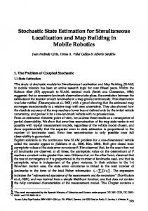
Figure 1. The Structure of the SLAM problem. A vehicle takes relative observations of environment landmarks. The absolute location of landmarks and vehicle are unknown.
Map Management for Efficient SLAM
is adopted. Although vehicle motion and the observation of landmarks is almost always non-linear and asynchronous in any real navigation problem, the use of linear synchronous models does not affect the validity of the proofs in Section 4 other than to require the same linearization assumptions as those normally employed in the development of an extended Kalman filter. The implementation of the SLAM algorithm described in Section 5 uses non-linear vehicle models and non-linear asynchronous observation models. The state of the system of interest consists of the position and orientation of the vehicle together with the position of all landmarks. The state of the vehicle at a time step k is denoted xv (k). The motion of the vehicle through the environment is modeled by a conventional linear discrete-time state transition equation or process model of the form xv (k + 1) = Fv (k)xv (k) + uv (k + 1) + vv (k + 1), (1) where Fv (k) is the state transition matrix, uv (k) a vector of control inputs, and vv (k) a vector of temporally uncorrelated process noise errors with zero mean and covariance Qv (k) (see Bar-Shalom and Fortman (1988) and Maybeck (1982) for further details). The location of the ith landmark is denoted pi . The “state transition equation” for the ith landmark is pi (k + 1) = pi (k) = pi ,
. . . pNT
...
�T
(3)
pTN
�T
xv (k + 1) p1 .. . pN
Fv (k) 0 0 I p1 = .. .. . . 0 0
... ... .. . 0
I pN
(6)
2.2.
The Observation Model
The vehicle is equipped with a sensor that can obtain observations of the relative location of landmarks with respect to the vehicle. Again, without prejudice, observations are assumed to be linear and synchronous. The observation model for the ith landmark is written in the form zi (k) = Hi x(k) + wi (k) = H pi p − Hv xv (k) + wi (k)
(7)
where wi (k) is a vector of temporally uncorrelated observation errors with zero mean and variance Ri (k). It is important to note that the observation model for the ith landmark is written in the form
= [−Hv , Hmi ]
(8) (9)
This structure reflects the fact that the observations are taken from on-board the vehicle and are therefore a measurement of some relative relationship between the vehicle and the feature. This relative relationship is often in the form of relative location, or relative range and bearing (see Section 5). The Estimation Process
(4)
xv (k) 0 p1 . 0 ..
0
x(k + 1) = F(k)x(k) + u(k + 1) + v(k + 1)
where I pi is the dim( pi ) × dim( pi ) identity matrix and 0 pi is the dim( pi ) × dim( pi ) null matrix.
2.3.
.
The augmented state transition model for the complete system may now be written as
(5)
Hi = [−Hv , 0 · · · 0, H pi , 0 · · · 0]
The augmented state vector containing both the state of the vehicle and the state of all landmark locations is denoted � x(k) = xvT (k) p1T
vv (k + 1) uv (k + 1) 0 0 p1 p1 + .. .. + . . 0 pN 0 pN
(2)
since landmarks are assumed stationary. Without loss of generality the number of landmarks in the environment is arbitrarily set at N . The vector of all N landmarks is denoted � p = p1T
269
pN
In the estimation-theoretic formulation of the SLAM problem, the Kalman filter is used to provide estimates of vehicle and landmark location. We briefly summarize the notation and main stages of this process as a necessary prelude to the developments in Sections 4 and 5 of this paper. Detailed descriptions may be found in Bar-Shalom and Fortman (1988), Maybeck (1982), and Leonard and Durrant-Whyte (1992). The Kalman filter recursively computes estimates for a state x(k)
270
Dissanayake et al.
which is evolving according to the process model in Eq. (6) and which is being observed according to the observation model in Eq. (7). The Kalman filter computes an estimate which is equivalent to the conditional mean xˆ ( p | q) = E[x( p) | Zq ]( p ≥ q), where Zq is the sequence of observations taken up until time q. The error in the estimate is denoted x˜ ( p | q) = xˆ ( p | q)−x( p). The Kalman filter also provides a recursive estimate of the covariance P( p | q) = E[˜x( p | q)˜x( p | q)T | Zq ] in the estimate xˆ ( p | q). The Kalman filter algorithm now proceeds recursively in three stages: 2.3.1. Prediction. Given that the models described in Eqs. (6) and (7) hold, and that an estimate xˆ (k | k) of the state x(k) at time k together with an estimate of the covariance P(k | k) exist, the algorithm first generates a prediction for the state estimate, the observation (relative to the ith landmark) and the state estimate covariance at time k + 1 according to xˆ (k + 1 | k) = F(k)ˆx(k | k) + u(k)
(10)
zˆ i (k + 1 | k) = Hi (k)ˆx(k + 1 | k)
(11)
P(k + 1 | k) = F(k)P(k | k)F (k) + Q(k),
(12)
T
respectively. 2.3.2. Observation. Following the prediction, an observation zi (k + 1) of the ith landmark of the true state x(k + 1) is made according to Eq. (7). Assuming correct landmark association, an innovation is calculated as follows νi (k + 1) = zi (k + 1) − zˆ i (k + 1 | k)
(13)
together with an associated innovation covariance matrix given by Si (k + 1) = Hi (k)P(k + 1 | k)HiT (k) + Ri (k + 1). (14) 2.3.3. Update. The state estimate and corresponding state estimate covariance are then updated according to: xˆ (k + 1 | k + 1) = xˆ (k + 1 | k) + Wi (k + 1)νi (k + 1) (15) P(k + 1 | k + 1) = P(k + 1 | k) − Wi (k + 1) × Si (k + 1)WiT (k + 1)
(16)
Where the gain matrix Wi (k + 1) is given by Wi (k + 1) = P(k + 1 | k)HiT (k)Si−1 (k + 1)
(17)
The update of the state estimate covariance matrix is of paramount importance to the SLAM problem. It is shown in Dissanayake et al. (2001) that as the vehicle progresses through the environment the errors in the estimates of any pair of landmarks become more and more correlated. Furthermore, the entire structure of the SLAM problem critically depends on maintaining complete knowledge of the cross correlation between landmark estimates. Minimizing or ignoring cross correlations is precisely contrary to the structure of the problem. 3.
Managing Complexity
A number of potential methods by which the growth of the computational burden imposed by the covariance update can be regulated have been described in the literature. This section examines a number of these methods, touching on their major strengths and weaknesses. Many of these approaches have been motivated by the search for an efficient method for maintaining consistent estimates of the map states without performing a complete update of the covariance matrix with each observation. The traditional SLAM algorithm requires such an update and it is well known that this step makes the filter difficult to implement in real-time for large maps. Present solutions to this problem can be divided into three broad categories. Some work has concentrated on the reduction in complexity that can be achieved by concentrating on fewer landmarks using active sensing. Other work has examined the possibility of applying sub-optimal update steps to once again reduce the complexity of updating the state covariance matrix. Finally, a number of researchers have proposed alternative map representations that change the manner in which information is added to the maps. 3.1.
Limiting the Number of Features
One method for improving the algorithm’s performance is to limit the number of features that are included in the map. Active sensing, in which a sensor is controlled to look at only a limited part of the environment, is one way of limiting the number of features to
Map Management for Efficient SLAM
be considered for inclusion in the map. To use active sensing effectively features that are likely to remain visible during the vehicle’s motion must be identified. An effective metric for the value of new landmarks may therefore come from the geometric distribution of landmarks as a function of the current vehicle trajectory. In Davison’s thesis (Davison, 1998) it is shown that active sensing can be performed to concentrate on a few, reliable features using a vision sensor mounted on an active pan tilt head. Accurate SLAM is shown to be possible despite the fact that not all of the considerable information contained in the visual images is used. The work in this paper falls under this category of map management approaches. It will be shown that features can be deleted from the map after the vehicle has left an area to once again limit the growth of the size of the map.
initial position have large covariances which are not much improved when the vehicle returns to its initial position. This large covariance can make data association difficult and may not allow the map estimates to converge. 3.2.2. Partitioned Update. Guivant and Nebot (2001) have recently proposed a simplification to the update step of the SLAM filter that can significantly reduce its computational complexity. Their main insight comes from the fact that the update of a large proportion of the features in the map is insignificant. This fact leads them to update only a select subset of the map features during a particular observation, reducing the computational burden to O(N ), where N is the number of states in the map. This results in a significant improvement in computational effort for large maps. 3.3.
3.2.
271
Alternative Map Representations
Sub-Optimal Updates
As an alternative to limiting the number of features in a map, the use of sub-optimal or near-optimal covariance updating schemes has also been considered. Conservative covariance update techniques can be shown to improve the computational performance of a SLAM algorithm at the expense of some loss of information. 3.2.1. Covariance Intersect. Uhlmann et al. (1997) have proposed a conservative algorithm for combining state estimates and computing an updated covariance matrix without a priori knowledge of the correlations between states. This approach substantially decreases the computational complexity of the SLAM problem using the covariance intersect (CI) method. The CI method does not require knowledge of the cross-correlations between states and only the diagonal elements of the state covariance matrix need to be maintained. Each observation is conservatively fused into the estimated state matrix through the use of the covariance intersect algorithm. This approach provides a computationally efficient mechanism for performing SLAM but discards a considerable amount of information contained in the covariance between the feature state estimates. This information usually allows improvements in the vehicle and map estimates to be be propagated throughout the map when a well-known feature is observed and is the key to the convergence properties of the algorithm. As shown in Uhlmann et al. (1997), feature estimates taken far from the vehicle’s
Much work in recent years has concentrated on the effect of the map representation on both the computational complexity of the SLAM algorithm and on the achievable estimation accuracy. In this section, a number of alternative map representations will be described. The significant characteristics of each of these representations will be discussed. 3.3.1. Relative Maps. In his thesis, Csorba proposed using the relative position between features rather than their absolute position as state variables (Csorba, 1997; Csorba and Durrant-Whyte, 1997). The relative location between landmarks is clearly independent of any absolute coordinate frame and of the location of the vehicle during an observation. Consequently, relative location estimates are uncorrelated. The covariance matrix is therefore diagonal and each observation can be fused into the filter by only updating the estimate of the relative state being observed. Newman developed this idea further and showed that while the relative representation is computationally efficient, it can result in inconsistent estimates of the relative states (Newman, 1999). For example, given estimates of the relative position between three landmarks, these independent estimates may not be mutually consistent. Newman proposed the Geometric Projection Filter (GPF) as a mechanism with which to enforce the consistency of the relative state estimates. By applying constraints to the relative states, Newman was able to recover a consistent map estimate at appropriate intervals at the cost of introducing correlations
272
Dissanayake et al.
between the states. It was suggested that the relative state estimates be maintained in one filter and that at appropriate intervals the constraints be applied to recover a consistent map. This consistent map could then be used for reasoning about the state of the map. New observations were fused into the original, relative map as they were received by the filter and the process of applying the constraints repeated at appropriate intervals to recover the consistent map. Newman also pointed out a number of difficulties that may arise from the relative representation of the map states. In particular, data association is potentially very difficult using a relative state representation. 3.3.2. Submaps. Another possibility is to divide a large map into a series of smaller submaps in order to reduce the computational complexity of the covariance update step. This approach has been adopted by a number of researchers. Chong and Kleeman (1998) have proposed a submap strategy whereby a number of independent, local submaps are generated as the vehicle operates. Estimates of the relative position between the submaps are maintained and a search algorithm is instantiated to relocalize the vehicle when the vehicle estimate has a high likelihood of being in the area of a previous local submap. This hierarchical approach to the mapping problem is shown to drastically reduce the memory and processing time requirements when compared with the global approach to SLAM. Chong and Kleeman do not provide methods for generating a globally consistent map of the environment. They suggest that this might be a possible extension to their work and might be accomplished using a least squares formulation. In Williams (2001) it is shown that globally consistent maps of the environment can in fact be generated through the use of appropriately formulated constraints. A computationally efficient method for SLAM using a number of globally referenced submaps is presented by Feder (1999) and Leonard and Feder (1999a). In this scheme, the submaps are allocated in an a priori manner and a unique vehicle state is associated with each submap. Methods are presented for transitioning the vehicle state estimates from one submap to another in a conservative manner. Finally, recent work by Castellanos et al. has introduced another method of performing SLAM (Castellanos et al., 1999) using global and local frames of reference in the mapping process. Feature sets are
estimated with respect to landmark frames, themselves estimated in the global frame of reference. Constraints between the various frames of reference are then used to generate a consistent global estimate of the vehicle state. A unique vehicle estimate is maintained with respect to each of the landmark frames. These distinct vehicle estimates are then fused together, using constraints, to recover a consistent estimate of the map states.
4.
Map Management by Deleting Landmarks
This section develops the theoretical basis of a map management strategy that significantly reduces the computation requirements for SLAM. It is shown that it is indeed possible to remove a large percentage of the landmarks from the map without making the map building process statistically inconsistent. Furthermore, it is shown that the computational cost of the SLAM algorithm can be reduced by judicious selection of landmarks to be preserved in the map. It is shown that a landmark estimate can be deleted from the map without affecting the statistical consistency of the underlying estimation process. Once deleted, all information accumulated so far about the landmark needs to be discarded and that the landmark must be re-initialized when it comes back into view. A process for selecting the landmarks to be removed is proposed. The proposed map management strategy can be used in conjunction with any one of the techniques described in Section 3 to further reduce the computational cost of implementing the SLAM algorithm.
4.1.
Evolution of the State Covariance Matrix
This section examines in detail, the evolution of the state covariance matrix P(k) that results from the special structure of the matrix Hi (k) give in Eq. (8). The state covariance matrix at any instant k may be written as P(k | k) = E[(x(k) − xˆ (k | k))(x(k) − xˆ (k | k))T | Zk ]. (18) This defines the mean squared error and error correlations in each of the state estimates. For the case of the SLAM filter, the covariance matrix takes on the
Map Management for Efficient SLAM
following form
Pvv (k | k)
PT (k | k) v1 P(k | k) = .. .
T Pvn (k | k)
Pvn (k | k)
Pv1 (k | k)
...
P11 (k | k) .. .
... .. .
P1n (k | k) .. .
T P1n (k | k)
...
Pnn (k | k) (19)
Pvv (k | k) = E[(xv (k) − xˆ v (k | k))
Pii (k | k) = E[(xi (k) − xˆ i (k | k))(xi (k) (21)
represent the landmark covariance, Pvi (k | k) = E[(xv (k) − xˆ v (k | k))(xi (k) − xˆ i (k | k))T | Zk ]
(22)
represents the cross-covariance between the vehicle and landmark estimate and Pi j (k | k) = E[(xi (k) − xˆ i (k | k))(x j (k) − xˆ j (k | k))T | Zk ]
� � Wi j = −Pv j HvT + Pi j HTpi Si−1 , j = v, 1, 2, . . . , n � � � � δP jl = −Pv j HvT + P ji HTpi Si−1 −Hv Pvl + H pi Pli , j = v, 1, 2, . . . , n; l = v, 1, 2, . . . , n (25)
(20)
represents the vehicle covariance,
− xˆ i (k | k))T | Zk ], i ∈ {1 . . . n}
During the update stage that follows the observation of landmark i, the Kalman gains and the change to the state covariance matrix can be written as
The effect of the observation of a given landmark i on the evolution of the vehicle and landmarks states and the state covariance matrix can now be summarized as follows
where
× (xv (k) − xˆ v (k | k))T | Zk ]
273
(23)
represents the cross-covariance between landmarks. The covariance matrix can be written more concisely using Pmm (k | k) to represent the map covariance and Pvm (k | k) to represent the cross-covariance between the vehicle and the map.
� Pvv (k | k) Pvm (k | k) P(k | k) = (24) T Pvm (k | k) Pmm (k | k) Dropping the index k for clarity and using Eq. (8) in Eq. (14), the innovation covariance after the ith landmark is observed is given by Si = Hv Pvv HvT − H pi Pvi HvT − Hv Pvi HTpi + H pi Pvi HTpi Clearly Si is a function of the covariances and cross-covariance of the vehicle and landmark i, and is independent of all other landmark covariances and cross-covariances.
– The Kalman gains associated with the vehicle state and all the landmark states are non-zero. Therefore, the estimate of all the landmark states are updated even when many of these landmarks are not visible from the current robot location. – All the elements of the state covariance matrix need to be modified after each observation. It is not sufficient to update the elements of the state covariance matix corresponding to the vehicle and the landmark currently being observed. This is the main reason for the computational complexity of the SLAM process. – The Kalman gain and the changes to the elements of the state covariance matrix associated with the jth landmark are a function of the covariances and crosscovariances associated with the vehicle state and the landmark states i and j. These updates are independent of the covariances and cross-covariances of all other landmark states. – Updates of the vehicle and landmark states and the associated covariance matrix after the observation of a landmark i are unaffected by the removal of the state corresponding to any landmark j and the corresponding rows and columns of the state covariance matrix. Therefore, any landmark that is currently not being observed can be removed from the map without affecting the statistical consistancy of the map building process. – When a removed landmark is observed again, the vehicle location and the states of other landmarks can not be updated using the state and the associated covariances of the landmark at the instant it was removed. The cross covariances will not have been updated after it had been removed from the state matrix and the landmark estimate must therefore be reinitialized using the current observation. This step results in a loss of information for the filter.
274
Dissanayake et al.
The prime objective of the SLAM process is to maintain a good estimate of the vehicle location by observing and estimating the locations of landmarks. The information available at any instant for localization depends on the accuracy of the sensor and the accuracy of the location estimates of the landmarks visible from the vehicle. An important result of the structure of the SLAM covariance matrix is a diminishing return between the number of landmarks being observed and the quality of the vehicle estimate (Gibbens et al., 2000). The observation of many highly correlated estimates of landmark locations do not offer significant additional information to the filter. The main insight offered by this work is the fact that a few well chosen landmarks are sufficient to maintain the accuracy of the estimate of vehicle location. Removing landmark state estimates from the state matrix that are unlikely to contribute much information to the estimate of vehicle location can therefore serve to reduce the computational complexity of the filter.
4.2.
Procedure for Selecting Landmarks for Removal
Landmark estimates represent a summary of the information collected by the robot during exploration. When the number of landmarks to be maintained in the map is to be restricted, the geometrical distribution and visibility constraints of the these landmarks are an important consideration in their selection. It is important to maintain landmarks that are most likely to be visible when the robot revisits a previously explored region. By the nature of the SLAM algorithm, the covariance of a feature estimate is a monotonically decreasing function of the number of times a feature has been observed (Dissanayake et al., 2001). Features that have been observed most often in a particular region will therefore tend to have lower covariances than those that are not easily visible. This suggests that a measure of the covariance of a particular landmark is good criteria to decide whether to keep it in the map. Another important factor in the selection of landmarks for removal from the state matrix is their position relative to the anticipated future path to be undertaken by the vehicle. Areas that are less likely to be revisited should have less features maintained than those that are likely to be traversed again. Unfortunately, in the case of exploratory SLAM, the environment itself is largely unknown and hence paths through the environment can often not be predicted.
It is also important to consider the fact that landmark location estimates that are less correlated can provide more information to the system. In the limiting case, when two landmark location estimates are fully correlated, there is no advantage to be gained by maintaining both these landmarks in the map except for geometric or visibility considerations. Consider, for example, the case of a state vector consisting of a single vehicle state estimate and two fully correlated feature states. The observation of either feature yields an identical update to the system states. It is therefore possible to remove one of the feature states without losing information. In practice, however, it is difficult to quantify the information loss to the filter without knowing the vehicle path and future observation sequences a priori. Another important consideration in the design of a strategy for removing landmarks from the state vector is the computational effort involved with selecting the landmarks to be removed. Clearly this cost needs to be small so as not to offset the computational advantage gained in the SLAM process by deleting these landmarks. The following two step process is therefore proposed for selecting the landmarks for removal from the map. – Collect the set of landmarks SL that changed from visible to not visible over a time interval during which the vehicle traveled a predetermined distance dv . Select one landmark to be preserved in the map and remove all the remaining landmarks in SL . This will tend to distribute the preserved landmarks over the area traversed by the vehicle. The landmark density of the final map obtained will be closely related to dv although this cannot be effectively predicted as it will also be a strong function of the vehicle path through the environment. A suitable choice for dv is a function of the range, accuracy and the speed of the sensor used, the extent of process noise and the tradeoff between the localization accuracy required and the computational efficiency. Such an incremental process of deletion, to a large extent, eliminates the need to consider the effect of geometry in evaluating the landmarks for their information content. The alternative approach of selecting a given number of the “best” landmarks from all the landmarks that are not visible is clearly computationally prohibitive. – The next step is to select the landmark that has the maximum information content from the set of landmarks SL . This landmark now serves to localize the
Map Management for Efficient SLAM
vehicle when the vehicle revisits the region surrounding the landmark. The selected landmark should provide the best information to improve the estimate of the location of the vehicle when the landmark is observed from any position within this region. Clearly, a lower uncertainty in the location estimate of the landmark will result in a lower uncertainty of the estimate of vehicle location following an observation of the landmark. Therefore, it is proposed to use the reciprocal of the trace of the covariance matrix P j j of the landmark location where j is the landmark under consideration. Furthermore, the covariance of the landmark location estimates tend to be closely related to the number of times the landmark is observed. The proposed strategy therefore tends to select the most prominently visible landmark in a given region. 5.
Results
This section shows results of the application of these techniques both in a simulated environment and on a mobile robotic platform. The vehicle and observation models used in both of these cases are identical. 5.1.
Experimental Setup
The laser range finder is a time of flight device that scans the range to the surrounding environment within a planar sweep of 180◦ . It returns 361 range measurements in a single sweep, with a range resolution of 5 cm and an angular resolution of 0.5◦ . The vehicle is driven manually. Range scans are logged together with encoder information by an onboard computer system. Range scans are processed to obtain point landmarks corresponding to foreground points, edges and corners in the environment. In the evaluation of the SLAM algorithm, this information is employed without any a priori knowledge of landmark location to deduce estimates for both vehicle position and landmark locations. In the following, the vehicle state is defined by xv = [x, y, ϕ]T where x and y are the coordinates of the centre of the front wheel of the vehicle with respect to some global coordinate frame and ϕ is the orientation of the vehicle axis. The landmarks are modeled as point landmarks and represented by a cartesian pair such that pi = [xi , yi ], i = 1 . . . N . Both vehicle and landmark states are registered in the same frame of reference.
5.1.1. The Process Model. Figure 3 shows a schematic diagram of the vehicle in the process of observing a landmark. The following kinematic equations can be used to predict the vehicle state from the steering γ and
Figure 2 shows the test vehicle; a three wheeled vehicle fitted with a laser range finder as the primary sensor used in the experiments. Encoders are fitted to the drive and steering motors to provide a measure of the vehicle speed and vehicle heading.
Figure 2. front.
275
The test vehicle. The laser range finder is seen in the Figure 3.
Vehicle and observation kinematics.
276
Dissanayake et al.
velocity V of the front wheel; x˙ = V cos(ϕ + γ ) y˙ = V sin(ϕ + γ ) V sin(γ ) ϕ˙ = , L where L is the wheel-base length of the vehicle. These equations can be used to obtain a discrete-time vehicle process model in the form
x(k) + T V (k) cos(ϕ(k) + γ (k)) x(k + 1) y(k + 1) = y(k) + T V (k) sin(ϕ(k) + γ (k)) ϕ(k + 1) ϕ(k) + T V (k)Lsin(γ (k)) (26)
Figure 4. A view from the mobile robot at the test site. Foreground points detected correspond to the vertical metal rails seen.
for use in the prediction stage of the vehicle state estimator. The landmarks in the environment are assumed to be stationary point targets. The landmark process model is thus
�
� xi (k + 1) xi (k) = (27) yi (k + 1) yi (k) for all landmarks i = 1, . . . , N . Together, Eqs. (26) and (27) define the state transition matrix f(·) for the system. 5.1.2. Feature Extraction. Feature extraction is performed independently on each laser scan and makes the assumption that each scan is an instantaneous snapshot of the environment. It is assumed that the speed of the laser sweep is much faster than the speed of the vehicle such that the vehicle motion does not significantly distort the scan. This assumption is reasonable for these experiments as the scan sweep takes about 40 ms and the indoor robot moves at less than 0.5 m/s. Figure 4 shows a view of the environment as seen from the robot. Figure 5 shows the clusters generated and the landmarks detected in the scan taken at this location. Note that the photograph has a limited field of view while the laser scans 180◦ . The poles of the hand-rail correspond to some of the foreground points detected while the edges and corners correspond to the steps in the walls and the door (see Bailey et al. (1999) for further details). 5.1.3. The Observation Model. The feature detector used in the experiments returns the range ri (k) and
Figure 5. Clusters and features detected in the laser scan that correspond to 4. The dotted lines show the field of view of the camera. The region of the laser scan bounded by the dotted lines therefore correspond to the image shown in Fig. 4. ‘P’, ‘E’, and ‘C’ denote the foreground points, edges and corners respectively.
bearing θi (k) to a landmark i. Referring to Fig. 3, the observation model can be written as ri (k) = (xi − xr (k))2 + (yi − yr (k))2 + wr (k)
� yi − yr (k) θi (k) = arctan − ϕ(k) + wθ (k) xi − xr (k)
(28)
where wr and wθ are the noise sequences associated with the range and bearing measurements, and [xr (k), yr (k)] is the location of the radar given, in global coordinates, by xr (k) = x(k) + a cos(ϕ(k)) − b sin(ϕ(k)) yr (k) = y(k) + a sin(ϕ(k)) + b cos(ϕ(k))
Map Management for Efficient SLAM
277
Equation (28) defines the observation model hi (·) for a specific landmark. 5.1.4. Estimation Equations. Sections 2 and 4 in this paper employed only linear models of vehicle and landmark kinematics. However, the implementation described here requires the use of non-linear models of vehicle and landmark kinematics f(·) and non-linear models of landmark observation h(·). Practically an Extended Kalman Filter (EKF) rather than a simple linear Kalman filter is employed to generate estimates. The EKF uses linearized kinematic and observation equations for generating state predictions. The use of the EKF in vehicle navigation and the necessary assumptions needed for successful operation is well known (see for example the development in Durrant-Whyte (1996)), and is thus not developed further here. 5.1.5. Map Initialization. In any SLAM algorithm the number and location of landmarks is not known a priori. Landmark locations must be initialized and inferred from observations alone. The feature detector returns a significant number of potential landmarks but only the observations resulting from landmarks that remain stationary over a number of observations should be used in the estimation process. An algorithm described in Dissanayake et al. (2001) is used to deal with these issues. The algorithm uses two landmark lists to record “tentative” and “confirmed” targets. A tentative landmark is initialized on receipt of a range and bearing measurement. A tentative target is promoted to a confirmed landmark when it receives a sufficient number of hits. Once confirmed, the landmark is inserted into the augmented state vector to be estimated as part of the SLAM algorithm. The landmark state location and covariance is initialized from observation data obtained when the landmark is promoted to confirmed status. 5.2.
Figure 6. The simulation environment showing the desired vehicle trajectory and the landmarks randomly scattered through the environment.
Figure 6 shows a map of a simulated environment in which the vehicle is operating. As can be seen, the desired vehicle trajectory is approximately circular. The landmarks are randomly distributed throughout the environment and the vehicle takes noisy range/bearing observations to random features that fall within the range of its on-board sensor. The filter parameters used for the simulation are shown in Table 1. Figure 7 shows a comparison between the error in the estimate for the full SLAM case versus the error committed by the proposed map-management approach along with the 2σ confidence bounds for both cases. The global vehicle covariance grows large as the vehicle navigates around the loop. As the vehicle approaches its initial location, a large correction in the estimate and corresponding reduction in position uncertainty occurs just before 300 s as the vehicle observes a previously estimated landmark with low variance. While the proposed approach to SLAM yields a higher
Computer Simulation Results Table 1.
This section presents results of the application of the SLAM algorithm using a simulated environment. Simulation is useful for understanding and verifying the performance of the algorithm as the true vehicle and feature locations are available. This allows for comparison between the true state of the system and the estimates generated by the filter. During the deployment of a vehicle in a field environment, ground truth is often not available and it is more difficult to accurately verify the performance of the algorithm.
Simulation filter parameters.
Description Sampling period
Symbol t(k)
Value 0.1 s
Vehicle velocity std dev
σv
0.05 V(k)m/s
Vehicle steer angle std dev
σγ
0.005 rad
Range measurement std dev
σR
1.0 m
Bearing measurement std dev
σB
0.05 rad
Vehicle length
L
Sensor range
1.5 m 25 m
278
Dissanayake et al.
Figure 7. Errors in the vehicle state estimates together with the estimated 2σ covariance bounds are shown. The full SLAM covariance estimates (dark) are shown for the vehicle pose states (xv , yv , ψv ) together with the estimates generated by the map management strategy (light). The errors appear to be within the 95% confidence bounds defined by the 2σ gate showing that the filter is well tuned. Despite the fact that the filter has discarded considerable information in the removed map estimates, it is still able to maintain an accurate estimate of the vehicle pose.
Figure 8. The innovation sequences. The estimates appear to be zero-mean and white with approximately 95% of the innovations falling within the 2σ innovation covariances bounds, again demonstrating that the filter is well tuned.
vehicle covariance relative to maintaining the full map estimate, it is clear that the filter is still maintaining similar estimates of the vehicle location. The innovation sequences can also be examined to see whether they resemble those from a zero-mean, white noise process. This is clearly the case as shown in Fig. 8. Given that the true state models are known
in simulation, generating a well tuned filter is straight forward. For real systems, the models must often be tuned through an experimental process in order to work correctly, although careful modeling of sensors and the environment can help to produce a well matched filter. Figure 9 shows the floating point operations required by the algorithm. The computational burden
Map Management for Efficient SLAM
Figure 9. The floating point operations required for the prediction and update stages of the filters. The cumulative floating point operations clearly show the improvements realised using the map management strategy (light) when compared with computational effort required by the full filter (dark).
rises quadratically until all of the observable features have been incorporated into the map. The complexity of each update is then maintained. The cumulative floating point operations are linear once all the features have been incorporated into the map. For the proposed algorithm, on the other hand, each observation incurs a smaller computational cost associated with the update of the smaller number of landmark estimates resulting in a reduced overall cost for the filter. Finally, the maps generated by the two implementations of the algorithm can be examined to verify that the proposed map management strategy does, in fact, yield a very similar map. Figure 10 shows the two maps generated by the algorithm along with the actual position of the landmarks. As can be seen, the features within range of the vehicle (indicated by the dashed circle) are maintained in the map. Once the vehicle has left an area, most of the landmark estimates are removed from the filter. 5.2.1. Sensitivity Analysis. As the landmark selection strategy is primarily justified based on intuitive arguments, a study of the sensitivity of the algorithm to the methods used for selecting landmarks is necessary. A number of additional simulated runs where the distance, dv , over which the vehicle traveled prior to deleting landmarks was changed were run. This resulted in different numbers of stored landmarks and slight variations in the distribution of stored landmarks.
279
Furthermore, the effect of varying the criteria used for evaluating the information content of the landmarks was also investigated. The first series of trials saw the distance, dv , traveled prior to removing landmarks estimates changed. Initially, the range of the sensor, Rs , was used as dv . Figure 11 shows that using 12 Rs , Rs or 2Rs does not significantly change the covariance of the vehicle location estimate. It is clear that what is important is to leave some landmarks so that the vehicle is effectively relocated when it revisits previously explored regions. The precise number of landmarks to be sensed or their spacing only has a minor impact on the performance of the vehicle state estimate. The effect of changes to the criteria used for evaluating the information content was also examined. The criteria for selecting the landmark in SL to maintain was changed from the trace of the landmark state estimate to its determinant. The trace provides a measure of the extent of uncertainty in the states while the determinant is a measure of the volume of uncertainty. The results of these trials are shown in Fig. 12. The differences between the covariances generated using these two selection criteria and that of the full filter are again small. It is clear from these simulated results that the proposed map management strategy is statistically consistent while yielding significant computational savings. Furthermore, changes to the heuristics used for selecting landmarks for removal seem to have minimal impact on the vehicle location estimate. The proposed choice of the trace Pii as a measure of the information content of a landmark estimate therefore seems justified. More important factors arising in real world applications are likely to arise from visibility constraints and ambiguous data association. In the simulated runs shown it is assumed that all features are visible from any position within range of the vehicle’s sensor. In practice, an estimate of a landmark state that is unlikely to be seen in the future will not add any information to the filter and can be removed. 5.3.
Experimental Results
In this section a practical implementation of the proposed simultaneous localization and map building (SLAM) algorithm on the indoor robot shown in Fig. 2 is presented. This implementation serves to highlight the effectiveness of the proposed map management strategy.
280
Dissanayake et al.
Figure 10. (a) The final map estimates for the full SLAM algorithm. As can be seen, estimates exist for all features that have been within range of the vehicle’s sensor. (b) The final map estimates using the proposed map management strategy. The current range of the vehicle’s sensor is plotted as a dashed circle relative to the final vehicle position. As can be seen, the features that are still in range of the sensor are maintained in the map. Only selected landmarks estimates outside of the range of the sensor are maintained.
Map Management for Efficient SLAM
281
Figure 11. (a) Errors in the vehicle state estimates together with the estimated 2σ covariance bounds are shown. The full SLAM covariance estimates (dark) are shown for the vehicle pose states (xv , yv , ψv ) together with the estimates generated by the proposed map management strategy using three different distance criteria dv ( 12 Rs , Rs , 2Rs ). This graph shows that the three criteria yield very similar performance. (b) The differences between the covariances computed in the three trials and that of the full filter. As can be seen, there is no difference in the vehicle covariance estimates until the loop has been closed and it begins reobserving landmarks. The difference in the three covariances associated with the different values of dv are too small to be clearly identified.
282
Dissanayake et al.
Figure 12. (a) Errors in the vehicle state estimates together with the estimated 2σ covariance bounds are shown. The full SLAM covariance estimates (dark) are shown for the vehicle pose states (xv , yv , ψv ) together with the estimates generated by using the trace and determinant of the landmarks states to evaluate the information content of the landmarks. This graph shows that both of these criteria yield very similar performance. (b) The differences between the covariances computed by the two filters and that of the full filter. As can be seen, there is no difference in the vehicle covariance estimates until the loop has been closed and it begins reobserving landmarks. The difference in the covariances in the two trials are again small.
Map Management for Efficient SLAM
283
Figure 13. Vehicle path and the map obtained using the full SLAM algorithm.
Figure 13 shows the landmark map consisting of 148 landmarks and the path of the vehicle computed using the full SLAM algorithm that maintains the complete set of landmarks in the state vector. In this experiment the robot starts at the origin, remaining stationery for approximately 15 seconds and then is driven along the corridor partly shown in Fig. 4. The total duration of the test run is about 800 seconds. The vehicle path and the map generated by the full SLAM algorithm was taken to be the basis for comparison of the proposed map management strategy to the full SLAM algorithm. Although the true path of the vehicle was not available, the map was verified by measuring the relative locations of some of the landmarks. Furthermore, the full SLAM algorithm has previously been verified on a number of different environments (Dissanayake et al., 2001; Clark and Dissanayake, 1999; Guivant and Nebot, 2001). Figures 14 and 15 show the landmark maps maintained, at two different instances, by the algorithm described in this paper. In this example, landmarks that change from visible to invisible were collected over a time period during which the vehicle traveled 5 m. The visibility range of the sensor was set to 15 m. The number of landmarks maintained in the map changes as the vehicle moves. On the average, this strategy results in a map that contains about 70 landmarks resulting in about an 8 fold reduction in the computational effort. Figure 16 compares the vehicle location estimates obtained using the full slam and the proposed algorithm and shows that the differences are hardly noticeable. Furthermore, Fig. 17 shows the uncertainty of the vehicle location estimates generated by the full SLAM
Figure 14. Vehicle path and the map obtained using the proposed map management strategy after 200 seconds. The ‘*’ show the landmarks currently active whereas ‘�’ show the landmarks that are inactive.
Figure 15. Vehicle path and the map obtained using the proposed computationally efficient SLAM algorithm after 500 seconds. The ‘*’ show the landmarks currently active whereas ‘�’ show the landmarks that are inactive.
algorithm and using the map management strategy. The difference in the vehicle location uncertainty estimate is of the order of 0.025 m. This figure also shows a typical characteristic of the SLAM algorithm. The uncertainty of the location estimates gradually increase while the vehicle is exploring new regions. This
284
Dissanayake et al.
Figure 16. Vehicle path obtained using the full SLAM algorithm and the proposed computationally efficient SLAM algorithm.
and localization is presented. It is shown that deleting landmarks from the map does not compromise the statistical consistency of the SLAM algorithm. A strategy to select landmarks to be removed is described and additional criteria for evaluating the relative merits of a landmark estimate are presented. Simulation and experimental results show that removing suitably selected landmarks does not significantly increase the errors in the estimated vehicle location. However, the computational effort required for the SLAM process is significantly reduced. Even with the proposed landmark deletion strategy, the number of the landmarks present in the map gradually increase as the robot explores more new regions. The next logical step in this research area is to formulate a strategy to merge the proposed algorithm with the techniques described in Section 3 that aim to reduce the computational complexity of the SLAM algorithm.
Acknowledgments The authors wish to thank the anonymous reviewers for their valuable and thought provoking comments.
References
Figure 17. Standard deviation of the position estimated by the full SLAM algorithm and the proposed computationally efficient SLAM algorithm.
uncertainty is reduced when the vehicle revisits previously known landmarks. It is clear that the presence of a few well known landmarks are sufficient to maintain the accuracy of the vehicle location estimate.
6.
Conclusions
In this paper a map management strategy to increase the computational efficiency of the estimationtheoretic solution to the simultaneous map building
Bailey, T., Nebot, E., Rosenblatt, J., and Durrant-Whyte, H. 1999. Robust distinctive place recognition for topological maps. In International Conference of Field and Service Robotics, Pittsburgh, USA, pp. 347–352. Bar-Shalom, Y. and Fortman, T. 1988. Tracking and Data Association. Academic Press: New York. Castellanos, J., Montiel, J., Neira, J., and Tardos, J. 1999. Sensor influence in the performance of simultaneous mobile robot localization and map building. In Proc. 6th International Symposium on Experimental Robotics, Sydney, Australia, pp. 203–212. Chong, K. and Kleeman, L. 1998. Large scale sonarray mapping using multiple connected local maps. In Field and Service Robotics, A. Zelinsky (Ed.), Springer-Verlag: Berlin, pp. 507–514. Clark, S. and Dissanayake, G. 1999. Simultaneous localization and map building using millimeter wave radar to extract natural features. In Proc. IEEE Int. Conf. Robotics and Automation, Detroit, USA, pp. 1316–1321. Csorba, M. 1997. Simultaneous localization and map building. Ph.D. Thesis, University of Oxford. Csorba, M. and Durrant-Whyte, H. 1997. New approach to map building using relative position estimates. In Proc. of SPIE: Navigation and Control Technologies for Unmanned Systems II, Vol. 3087, The International Society for Optical Engineering, pp. 115–125. Davison, A. 1998. Mobile robot navigation using active vision. Ph.D. Thesis, University of Oxford.
Map Management for Efficient SLAM
Dissanayake, M., Newman, P., Clark, S., Durrant-Whyte, H., and Csobra, M. 2001. A solution to the simultaneous localization and map building (SLAM) problem. In IEEE Trans. Robotics and Automation, 17(3):229–241. Durrant-Whyte, H. 1996. An autonomous guided vehicle for cargo handling applications. Internation Journal of Robotics Research, 15(5):407–440. Feder, H. 1999. Simultaneous stochastic mapping and localization. Ph.D. Thesis, Massachusetts Institute of Technology, Dept of Mechanical Engineering. Gibbens, P., Dissanayake, M., and Durrant-Whyte, H. 2000. A closed form solution to the single degree of freedom simultaneous localization and map building (SLAM) problem. In Proc. IEEE Conference on Decision and Control, Vol. 1, pp. 191–196, IEEE. Guivant, J. and Nebot, E. 2001. Optimization of the simultaneous localization and map building algorithm for real time implementation. In IEEE Transactions on Robotics and Automation, 17(3): 242–257. Leonard, J. and Durrant-Whyte, H. 1992. Directed Sonar Sensing for Mobile Robot Navigation, Kluwer Academic Publishers: Norwell, MA. Leonard, J. and Feder, H. 1999a. A computationally efficient method for large-scale concurrent mapping and localization. In Ninth International Symposium on Robotics Research, Utah, USA, pp. 316–321. Leonard, J. and Feder, H. 1999b. Experimental analysis of adaptive concurrent mapping and localization using sonar. In Proc. 6th International Symposium on Experimental Robotics, Sydney, Australia, pp. 213–222. Maybeck, P. 1982. Stochastic Models, Estimation and Control, Vol. 1, Academic Press: New York. Newman, P. 1999. On the structure and solution of the simultaneous localization and map building problem. Ph.D. Thesis, University of Sydney, Australian Centre for Field Robotics. Uhlmann, J., Julier, S., and Csorba, M. 1997. Nondivergent simultaneous map building and localization using covariance intersection. In Proc. of SPIE: Navigation and Control Technologies for Unmanned Systems II, Vol. 3087, The International Society for Optical Engineering, pp. 2–11. Williams, S. 2001. Efficient solutions to autonomous mapping and navigation problems. Ph.D. Thesis, University of Sydney, Australian Centre for Field Robotics. Williams, S., Dissanayake, G., and Durrant-Whyte, H. 2001. Towards Terrain-Aided navigation for underwater robotics. Advanced Robotics, 15(5):533–550.
Gamini Dissanayake graduated in Mechanical/Production Engineering from the University of Peradeniya, Sri Lanka. He
285
received his M.Sc. in Machine Tool Technology and Ph.D. in Mechanical Engineering (Robotics) from the University of Birmingham, England in 1981 and 1985 respectively. He was a lecturer at the University of Peradeniya and the National University of Singapore before joining the University of Sydney, Australia, where he was attached to the Australian Centre for Field Robotics. He is now the Professor of Mechanical and Mechatronic Engineering at University of Technology, Sydney. His current research interests are in the areas of localization and map building for mobile robots, navigation systems, dynamics and control of mechanical systems, cargo handling, optimisation and path planning.
Stefan B. Williams received the B.A.Sc. degree (1st class honours) in Systems Design Engineering from the University of Waterloo in Waterloo, ON, Canada in 1997. He submitted his thesis in 2001 to complete the requirements for a Ph.D. in Mechatronic Engineering (Field Robotics) at the Australian Centre for Field Robotics (ACFR) in the School of Aerospace, Mechanical and Mechatronic Engineering at the University of Sydney, Australia. He is currently a Research Associate at the ACFR funded through BAe Systems in the UK. His current research interests focus on robotics and artificial intelligence and concentrate on the development of terrain-aided navigation techniques, sensor fusion and vehicle control architectures for real-time platform control.
Hugh Durrant-Whyte received the B.Sc. (Eng.) degree (1st class honours) in Mechanical and Nuclear Engineering from the University of London, U.K., in 1983, the M.S.E. and Ph.D. degrees, both in Systems Engineering, from the University of Pennsylvania, U.S.A., in 1985 and 1986, respectively. From 1987 to 1995, he was a Senior Lecturer in Engineering Science, the University of Oxford, U.K. and a Fellow of Oriel College Oxford. Since July 1995 he has been Professor of Mechatronic Engineering at the Department of Mechanical and Mechatronic Engineering, the University of Sydney, Australia, where he leads the Australian Centre for Field Robotics, a Commonwealth Key Centre of Teaching and Research. His research work
286
Dissanayake et al.
focuses on automation in cargo handling, surface and underground mining, defence, unmanned flight vehicles and autonomous sub-sea vehicles.
Tim Bailey received his B.E. in Mechanical & Mechatronic Engineering at the University of Sydney in 1997. He commenced his
Ph.D. at the Australian Centre for Field Robots at the University of Sydney later in 1997 and is currently completing his thesis on allterrain outdoor navigation for mobile robots. His research interests include mobile robot localization and mapping, Bayesian estimation techniques, and probabilistic sensor modeling.