Inverse Distance is fast but has the tendency to generate âbull's-eyeâ patterns of ... The results of present research show that most of above mentioned methods ...
Mapping Precipitation Variability Using Different Interpolation Methods Nina Nikolova , Stanislav Vassilev Faculty of Geology and Geography, University of Sofia “St. Kliment Ohridski” Sofia, BULGARIA
Abstract Precipitation data are available from recording stations that present point samples. Spatial interpolation may be used to estimate precipitation at unsampled sites. The present analysis is based on the annual precipitation totals observed at Danube Plain, Bulgaria. Precipitation variability is presented by deviation of annual precipitation totals. The investigated period is 2000 - 2004 and the reference period is 1961-1990. The paper demonstrates the implementation of different interpolation methods into meteorological data analysis.. Keywords: spatial interpolation, annual precipitation, Danube Plain
Introduction Meteorological stations are located in the places which are often not of interest for different human activity. The value of climate elements can not be measure in all point of the territory but only in sample points. Spatial interpolation may be used to estimate the values in such areas where there is not measurement. Many research works show the importance of interpolating values of climate variables from stations to large areas. Most of investigations consider the spatial modeling and mapping of temperature variables (Willmott and Matsuura, 1995, Holdaway, 1996, Kurtzman and Kadmon, 1999; Gigov and Nikolova, 2002). Some methods for precipitation interpolation are presented by Sárközy, 2000. The precipitation is a key element of climate, which determines the availability of drinking water and the level of the soil moisture. Changes in precipitation could have a significant impact on society. Because of this it is important to have information about precipitation and its spatial distribution and variability not only in sample point but also in all point of the territory. The aim of the present paper is to demonstrate the implementation of different methods for interpolation of climate data on the example of precipitation data. The advantages and restrictions of some methods for creation of statistical surfaces are presented.
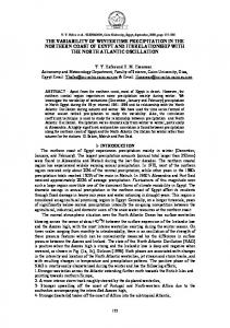
Study area Geographical features of the territory The Danube Plain is the most northern part of Bulgaria. It is territory is 31 522 km2 and represent 24% of entire area of the country (fig.1.). The relief here is uniform and is compound mainly by lowlands and hills. The maximum elevation is 502 m and average is 178 m. Climate of Danube Plain is moderate continental. Because of the plain relief the air masses from north, west, and east flow easily into the territory. Some local geographical peculiarities as Black Sea on the east and Balkan Mountains on the south modify the climate. The Balkan Mountains has a barrier effect on air masses. On the average, north part of Bulgaria is about one or two degree cooler and receives more precipitation than southern Bulgaria. The main cause for precipitation distribution in the country is atmospheric circulation which is influenced considerably by orography. Average precipitation in Bulgaria is about 600 mm per year but in northeast part and the Black Sea coastal area the annual precipitation total is 500 or less than 500 mm.
Investigated area Fig.1. Location of the investigated area Data used for the research The present analysis is based on the annual data for precipitation totals from 11 meteorological stations which are situated in Danube plain, Bulgaria. The sources of data are meteorological yearbook published by the National Institute of Meteorology and Hydrology, Sofia, Bulgaria, Statistical Yearbook of the National Statistical Institute, Bulgaria and the bulletins of Executive Environmental Agency, Bulgaria. In order to mapping precipitation values the data from five Romanian meteorological stations situated near to Bulgarian-Romanian border are used. The data from some Bulgarian station stations which are situated outside of the Danube Plain are also taken for the interpolation. The stations are listed in Table 1. Table 1. Meteorological stations in Bulgaria under the present study Meteorological stations
Latitude
Longitude
Elevation (m)
Vidin Lom Oryahovo Kneja Pleven Rousse Rasgrad Shoumen Dobrich Varna StaroOryahovo Veliko Tyrnovo Vraca Belogradchik Drobeta Turnu Severin Craiova Rosiorii de Vede Calarasi Constanta
43° 39' 43° 49' 43° 44 43° 30' 43° 25' 43° 51′ 43° 32' 43°16' 43° 34' 43° 12' 42° 59' 43° 05' 43° 12' 43° 37' 44° 38' 44° 19' 44° 06' 44° 12' 44° 13'
22°53' 23° 14' 23°58 24°05' 24°35' 25° 58′ 26° 31' 26°56' 27°50' 27°55' 27°48' 25°38' 23°32 22°41' 22°38' 23°52' 24°59' 27°12' 28°38'
37 21 31 120 133 87 183 216 235 12 14 194 548 545 77 192 102 19 13
Precipitation variability is presented by deviation (in %) of annual precipitation totals for period 19611990. This period is determined form the World Meteorological Organization as a current climate. The utilization of interpolation methods is shown by mapping of precipitation variability for 2000 (dry year) and for 2002 (wet year). Many research works (Alexandrov et all, 2004, 2005) show that the drought in 2000 is very characteristic of most part of Bulgaria. In many meteorological stations the annual precipitation in this year did not reach even 60% of the climate values for the period 1961-1990 (Alexandrov, V. 2004). As the wet year the authors consider 2002. In all of investigation stations in this year the annual precipitation exceed the average values for 1961-1990. In some stations the deviation is about 150%. Peculiarities of climate data in view of interpolation In this part the comparison between interpolation of climate data and one for the relief will be done. Some of peculiarities of climate data which have to be taken into consideration at interpolation will be presented: Usually the interpolation of climate data is made on the base of limited number of points. The functions of interpolation are used for predicting values of climate elements on the large territory between the points of measurement. Whereas for the relief many points (hundreds or thousands) are used for the interpolation. We can not choose the places of points for the interpolation. Generally the extremely values of elements have not the same situation as meteorological stations. The values measured at the meteorological stations are the local maxima or minima at the interpolation and this fact is often mislead. The interpolation of the relief is made on the base of selected data which are representative for structural lines and typical points of the relief. Possibility for utilization of data from territory outside investigated region. It is of great importance to have some points outside of chosen territory. There are limitations when the region has a common border with the sea. Lack of big distinction between the values from different stations is characteristic of climate data. This fact requires avoiding the methods which have tendency to creation of ‘bull’s-eye’. It is necessary to use the methods which make smooth the surface. In contrast to this sharply changes of the slops and peaks are often observed at the relief. Most of systems for the interpolation are not supported breaking at the created surface. These breakings are necessary at relief modeling, for example on the borders of water areas, at very steep slops or vertical wall. The fact that climate data are in all parts of the territory gives the possibility for utilization of all systems for interpolation. There are some factors which often are not taken into consideration at the interpolation. The climate is determined by many factors as relief, water basins, type of vegetation etc. Because of this the interpolated data are burden with some errors. To avoid these errors it is necessary to include additional data but this is not always possible. The precise selection of side-factors for interpolation of climate data should be done. Methods for interpolation
The methods for interpolation are chosen on the base of existing research works (Collins F et all, Sárközy, 2000, Yang et al., 2004) and availability of investigated data. Survey of methods Interpolation methods allow creating a surface on the base of sample points and predicting of values in all point of territory. There are many interpolation methods which produce different results using the same data. The methods can be divided at two main groups: Regular and Irregular. In case of using the irregular methods the points are connected at triangles. Each triangle determines a surface which is used for assessment of values of each point. It is necessary to have many known points for irregular methods implementation. Because of this these methods are not suitable for climate data interpolation. These methods are often used at relief modeling. The regular methods for interpolation make close initial points and create a net of identical rectangles with determined by user sides. In this case two main groups of methods can be used: deterministic and geostatistical. The mathematic methods (relations) are used by deterministic methods. Geostatistical methods are based on the mathematic and statistical functions which can be used for generation of surfaces and forecasts assessment.
The Surfer software is used in the present research. This program supports the following interpolation methods (Louie, 2001): Inverse Distance is fast but has the tendency to generate “bull's-eye” patterns of concentric contours around the data points. Kriging is one of the more flexible methods and is useful for gridding almost any type of data set. With most data sets, Kriging with a linear variogram is quite effective. For larger data sets, however, Kriging can be rather slow. Minimum Curvature generates smooth surfaces and it is fast for most data sets. Nearest Neighbor. When the data is a nearly complete grid with only some missing holes, this method is useful for filling in the holes, or creating a grid file with the blanking value assigned to those locations where no data is present. Being most useful for nominal data, it produces a highly discontinuous interpolation map. Polynomial Regression processes the data so that underlying large scale trends and patterns are shown. This is used for trend surface analysis. Polynomial Regression is very fast for any amount of data, but local details in the data are lost in the generated grid. Radial Basis Functions is quite flexible, and like Kriging, generates among the best overall interpretations of most data sets. This method produces results that are quite similar to Kriging. Shepard's Method is similar to Inverse Distance but does not tend to generate "bull's eye" patterns, especially when a Smoothing factor is used. Triangulation with Linear Interpolation is fast with all data sets. When you use small data sets Triangulation generates distinct triangular facets between data points. One advantage of triangulation is that, with enough data, triangulation can preserve break lines defined in a data file. The results of present research show that most of above mentioned methods are not suitable for climate data interpolation. The good results have been obtained at utilization of the following methods: Kriging, Minimum curvature and Radial Basis Function. We are going to consider these methods at the following section. Kriging Kriging is a geostatistical gridding method which is proven, useful and popular in many fields. This method sets the weight of each sample point according to the distance between the point to interpolate and the sample points. Kriging’s procedure estimates this dependence over the semivariance, which takes different values according to the distance between data items. The function that relates semivariance to distance is called semivariogram1 and shows the variation in correlation among the data, according to distance (García-León, Felicísimo, Martínez 2004) There are three factors that are uniquely incorporated in the Kriging method: Variogram Model, the Drift Type and the Nugget Effect. The variogram model mathematically specifies the spatial variability of the data set and the resulting grid. The interpolation weights, which are applied to data points during the grid node calculations, are direct functions of the variogram model. Surfer supports seven common variogram functions: Spherical, Exponential, Linear, Gaussian, Hole-Effect, Quadratic, and Rational Quadratic. For climate data interpolation the best results are obtained using Linear, Quadratic and Exponential variogram functions. In comparison to linear function as fewer are the points for the interpolation as better are the results in case of using the Quadratic and Exponential variogram functions. There are two perimeters at each function: Scale (C) and Length (A). Тhe Scale parameters define the sill for the variogram components. In most situations, the variogram model sill is approximately equal to the variance of the observed data. The Length (A) parameters define how rapidly the variogram components change with increasing separation distance. The Length (A) parameter for a variogram component is used to scale the physical separation distance. For the Spherical and Quadratic variogram functions, the Length (A) parameter is also known as the variogram range. Surfer offer implicit values for Scale and Length which lead to satisfied results at the interpolation. Тhe Drift Type will have a significant effect during gridding when interpolating across large holes in the data distribution pattern, and when extrapolating beyond the limits of the data. When the data points 1 The variogram is a function which connects discrepancy of the point data and a distance between them. It can be used for representation of spatial correlation between the data and for the visualization of values of discrepancy in the data before generation of the surface.
are evenly dispersed within the area of interest, the Drift Type option has little effect on the generated grid. Three drift options are available in Surfer: No Drift, Linear Drift, and Quadratic Drift. The No Drift option meaning that the interpolation uses “Ordinary Kriging”. No Drift is appropriate when the data is evenly dispersed. The Linear Drift and Quadratic Drift options are used to implement "Universal Kriging". The use of linear or quadratic drift should be based upon knowledge of an underlying trend of the data. If the data tends to vary around a linear trend, then the Linear Drift option is most appropriate. If the data tends to vary around a quadratic trend (e.g. a parabolic bowl), then the Quadratic Drift option is most appropriate. (Louie 2001) The Nugget Effect is used when there are potential errors in the collection of the data, or when the sample sizes for data are too small to provide statistical significance. Specifying a nugget effect causes Kriging to become more of a smoothing interpolator, implying less confidence in individual data points versus the overall trend of the data. As you increase the nugget effect, data points are not honored as closely. The Error Variance edit box allows you to specify the variance of the measurement errors. This value is a quantification of the repeatability of the data measurements. The Micro Variance edit box allows you to specify the variance of the small scale structure. (Louie 2001) Minimum Curvature The minimum curvature method is widely used in the earth sciences. The interpolated surface generated by Minimum Curvature is analogous to a thin, linearly-elastic plate passing through each of the data values with a minimum amount of bending. Minimum Curvature generates the smoothest possible surface while attempting to honor your data as closely as possible. Minimum Curvature is not an exact interpolator however. This means that the data is not always honored exactly. Panchenko (1999) gives the following general equation for the method: (1 - T) * L (L (z)) + T * L (z) = 0 where T is a tension factor between 0 and 1, and L indicates the Laplacian operator. Minimum curvature can cause undesired oscillations and false local maxima or minima, and you may wish to use T > 0 to suppress these effects. Experience suggests T ~ 0.25 usually looks good for potential field data and T should be larger (T ~ 0.35) for steep topography data. T = 1 gives a harmonic surface (no maxima or minima are possible except at control data points). (Panchenko 1999) Radial base functions Radial Basis Functions are a diverse group of data interpolation methods. In terms of the ability to fit the data and to produce a smooth surface, the Multiquadric method is considered by many to be the best method. All of the Radial Basis Function methods are exact interpolators so they make an attempt to honor the data. You can introduce a smoothing factor to all the methods in an attempt to produce a smoother surface. (Louie 2001) Under most circumstances, the Multiquadric function is the most desirable. In this case the surface is calculated on the base of the following general equation:
F (d ij ) = d ij2 + r 2 where F(dij) is the radial base function, d - the distance between points; The function comprises an r parameter: the softening factor. This value should be previously tested according to the data in each case; a very high value will generate a very softened surface, far from the real surface (García-León, Felicísimo, Martínez 2004). The Radial Basis Functions support special parameter R2 which is a shaping or smoothing parameter. The larger the R2 parameter, the rounder and the smoother are the contour lines. There is no universally accepted method for computing an optimal value for this parameter. A reasonable trial value for R2 is between the average sample spacing and one-half the average sample spacing. (Louie 2001).
Results and discussion Spatial distribution of annual precipitation and its variability The spatial distribution of annual precipitation in 2000 and 2002 is presented on the figures 2, a) and b). One can see that in northwestern part of the Danube plain the annual precipitation in 2000 was about 300 mm. The values increase on the east and south and reach 400 mm. This kind of spatial distribution of precipitation is characteristic also for the year 2002. The annual precipitations in this
year increase from 600-650 mm in the western part to above 800 mm in some station in central and eastern part of the Danube plain. The cause for the lower precipitation in the western part is the impact of the South Carpathian Mountains and Balkan mountains which have a barrier effect on wet air masses blowing from north-west. The spatial distribution of the average precipitation for the period 1961-1990 is presented at fig. 2 c). a)
b)
c)
Fig. 2. Kriging interpolation of annual precipitation for: a) 2000; b) 2002; c) 1961-1990
Figure 3 shows the deviation of annual precipitation in 2000 from the average for the period 19611990. The maps are made by using different interpolation methods. Some discrepancy is occurred at the Minimum curvature interpolation (fig. 3b). The precipitations in 2000 are between 60 and 90 % of annual precipitation normals (1961-1990). The deviations of the annual precipitation normals are used by some authors (Slavov et al., 2000) to determine the intensity of drought – weak drought when the precipitation is 75% of the normals, average drought – from 50 to 75% and strong drought under the 50% of normals. The drought in 2000 is well expressed in the Northwestern part of the Danube plain (fig. 3). The annual precipitation here is between 50 and 60% of climate normals. Such values are characteristic also for the Romanian meteorological station situated near to this part. The drought in Northeastern part of Bulgaria is not clearly expressed. This fact has been shown by Velev (2000) for the period 1970-1999. For 2002 in all stations under observation, the annual precipitation was above the average for the period 1961-1990 (fig. 4.). The deviation in the western part is lower than in other parts of the Danube plain. The annual precipitation in 2002 is about 110 – 115% of climate normals in western part and rich about 150 % of climate normals in central and eastern part of the region. On the Black sea coast the deviation decreases and it is 120% of the normals. a)
b)
c)
Fig. 3. Deviation of annual precipitation in 2000 from the average for the period 1961-1990 a) Kriging, b) Minimum curvature, c) Radial Basis Function interpolation
a)
b)
c)
Fig. 4. Deviation of annual precipitation in 2002 from the average for the period 1961-1990 a) Kriging, b) Minimum curvature, c) Radial Basis Function interpolation Improvement of the results from interpolation Anisotropy Anisotropy during gridding implies a preferred direction, or direction of higher or lower continuity between data points. Anisotropy is applied by specifying an anisotropy ratio which states: "Give more weighting to points located along one axis versus points located along another axis." Alternatively you can say that points that lie farther away along one axis are given equivalent weights to points that lie
closer along the other axis. The relative weighting is defined by the anisotropy ratio. This possibility is very useful at the climate data interpolation on the large areas. This allows setting different impact of neighbor points. The climate belts are situated along the parallel. Because of this the points with the similar latitude have bigger influence than the points situated northern or southern. Anisotropy can be presented as an ellipse. The points from the long axis of the ellipse have bigger influence on the determination of interpolation value than the points situated along the short axis on the ellipse. At the isotropic models the circumference is used instead of ellipse. In this case all point around investigated one are with the same weight. The anisotropy is created by two parameters: angle of long axis and flatness of the ellipse (ratio). All methods form Surfer support anisotropy. An exception is the Minimum Curvature where the angle of long axis can not be set. It is reasonable to use anisotropy at our research because the elevation of the Danube plain increases from north to south and the point with most southern situation are form pre-mountainous part of the Balkan mountain. The weight of these points at the interpolation has to be lower that the influence of the points situated on the Danube plain. For this purpose the angle of anisotropy 0 and the ratio 1.2 are used Smoothing a Grid As was mentioned above the values of climate data modify gradually. Generally there are not big differences between the neighbor points. Because of this it is important to use the options at different interpolation methods which lead to smoothing the created surface and removing the abrupt changes. There is a special option for smoothing the created surface at the Surfer. Smoothing operations are used to even out angular contours and blocky surfaces, or to eliminate noise in a contour map or surface. Produced by some interpolation methods grid can be smoothed using Spline Smoothing or Matrix Smoothing. Spline Smoothing is most effective for eliminating angular contours or surfaces by filling in a sparse grid. The operation works at two ways: 1) the new points are placed between tow neighbor points. The number of new points is controlled by the user; 2) calculating of the grid at the new number points Matrix Smoothing is most effective for removing noise or variability between grid nodes that are close together. The general trends in the surface are retained, but spikes tend to be eliminated. Matrix smoothing results in an output grid with the same dimensions as the input grid. Matrix smoothing generates a blanked border around the outside of the grid. (Louie 2001) Each grid point is calculated as average of neighbor points Verification of the results The best method for verification of the interpolation is to use the experimental data. It is difficult to proof interpolation of climate data because of two reasons. First there are a limited number of meteorological stations which give information. The second, the values of climatic elements depend of many factors as elevation, relief, peculiarities of the landscape. The interpolation method and peculiarities of climate data both determined the discrepancy between measured and interpolated values. In regard of choice of interpolation method it is necessary the preliminary data analysis to be done. The results of the interpolation can be verified by comparison of different versions of the same method. It is possible to use different functions in the same interpolation method. If there is the big difference between the final results the interpolation method is not suitable or the data are not sufficient. This is observed often on the outlying of the investigated territory where the data are few. When big differences are observed at some part of the region using different functions from one method it is necessary to use additional data. If this data are not available the methods which give a minimal deviation from the data form neighbor region have to be used. At the present research the minimal deviations observed at the mapping using Kriging – linear, quadratic and exponential interpolation. The different results are obtained by other methods and this show that these methods are not suitable.
Conclusion The results of present research show that spatial interpolation may be used to estimate the values in such areas where there is not measurement. There are many interpolation methods which produce different results using the same data. The choice of the interpolation methods depends of number of measurement points and factors which determine the peculiarity of climate at the investigated territory. The good results have been obtained at precipitation interpolation by the following methods: Kriging, Minimum curvature and Radial Basis Function. The precipitations in 2000 are between 60 and 90 % of annual precipitation normals (1961-1990). The drought in 2000 is well expressed in the Northwestern part of the Danube plain where the annual precipitation is between 50 and 60% of climate normals. For 2002 in all stations under observation, the annual precipitation was above the average for the period 1961-1990 The deviation in the western part is lower than in other parts of the Danube plain.
Acknowledgements. The authors wish to thank most sincerely Dr. V. Alexandrov form National Institute of Meteorology and Hydrology, Bulgaria for useful discussion and Dr. A. Geicu and Dr. C. Boroneant from National Meteorological Administration, Romania for provision of climate data.
Reference Alexandrov, V. 2004: Climate Variability and Change and Related Drought on Balkan Peninsula BALWOIS, Ohrid, FY Republic of Macedonia, 25-29 May 2004). Alexandrov, V. and M.Genev, 2004. The effect of climate variability and change on water resources in Bulgaria. Proceedings of the British Hydrological Society Conference on Science and Practice for the 21st century, (CD version) 8 pp. Alexandrov, V., M.Genev and H.Aksoy, 2005 Climate variability and change effects on water resources in the western Black Sea coastal zone. Proceedings of the European Water Resources Association (EWRA’2005) Conference: “Sharing a common vision for our water resources”, 7-10 September 2005, Menton, France (in press) Collins F. C. Jr., P. V. Bolstad. A Comparison of Spatial Interpolation Techniques in Temperature Estimation.http://www.sbg.ac.at/geo/idrisi/gis_environmental_modeling/sf_papers/collins_fred/collins.h tml, accessed February 10 2006 Gigov A., M. Nikolova. 2002. Mapping Air Temperature Changes in Bulgaria Using GIS Spatial Analyses. Proceedings of the International Scientific Conference in Memory of Prof. Dimitar Yaranov, Varna, Bulgaria, 114-121. García-León, J.; A. M. Felicísimo, J. J. Martínez 2004. A methodological proposal for improvement of digital surface models generated by automatic stereo matching of convergent image networks. http://www.isprs.org/istanbul2004/comm5/papers/522.pdf accessed February 10 2006 Holdaway M.R. 1996: Spatial modeling and interpolation of monthly temperature using kriging. Climate Research, Vol. 6. pp 215-226. Kurtzman D., R. Kadmon. 1999: Mapping of temperature variables in Israel: acomparison of different interpolation methods. Climate Research, Vol. 13, pp 33-43 Louie, John N. 2001. Gridding Overview. http://www.seismo.unr.edu/ftp/pub/louie/class/333/contour/surfer.html accessed February 10 2006 Panchenko, I. 1999. The Generic Mapping Tool. http://xray.sai.msu.ru/~ivan/gmt/man/surface.html accessed February 10 2006 Sárközy F. 2000: GIS Function – Interpolation. http://www.agt.bme.hu/public_e/funcint/funcint.html , accessed February 10 2006 Slavov N., E. Koleva, V. Aleksandrov. 2000. Klimatichni osobenosti na zasushavaneto v Bulgaria. Bulgarian Journal of Meteorology & Hydrology, vol. 11, N 3-4, 100-113. (Climatic characteristics of drought in Bulgaria. Bulgarian Journal of Meteorology & Hydrology, vol. 11, N 3-4, 100-113) Velev, St. (2000). Globalnite promeni i klimatyt na Bulgaria. Sbornik ot dokladi. Mejdunarodna nauchna sesia 50 godini Geografski institut, Sofia, Bulgaria, 99-107. (Velev, St. Global changes and
climate of Bulgaria. Proceedings of the International scientific session 50 years Institute of Geography, Sofia, Bulgaria, 99-107, in Bulgarian). Willmott, C. J. and K. Matsuura, 1995: Smart Interpolation of Annually Averaged Air Temperature in the United States. Journal of Applied Meteorology, 34, 2577-2586. Yang Ch, Kao S., Lee F., Hung P. 2004. Twelve Different Interpolation methods: A Case Study of Surfer 8.0. Geo-Imagery Bridging Continents, XXth ISPRS Congress, 12-23 July 2004 Istanbul, Turkey. http://www.isprs.org/istanbul2004/comm2/papers/231.pdf , accessed February 10 2006