Marginal True-Score Measures and Reliability for Binary Items as a Function of Their IRT Parameters Dimiter M. Dimitrov, Graduate School of Education, George Mason University, Fairfax, Virginia
This article provides analytic evaluations of
contribution of IRT calibrated items to marginal
population true-score measures for binary items
true-score measures and may have valuable
given their item response theory (IRT) calibration.
applications in test development and analysis. For
Under the assumption of normal trait distribution,
example, given a bank of IRT calibrated items, one
the expected values of marginalized true scores,
can select binary items to develop a test with
error variance, true score variance, and reliability
known true-score characteristics prior to
for norm-referenced and criterion-referenced
administering the test (without information about
interpretations are presented as a function of the
raw scores or trait scores.) Calculations with the
item parameters. The proposed formulas have
proposed formulas are easy to perform using basic
methodological and computational value in
statistical programs, spreadsheet programs, or even
bridging concepts of IRT and true score theory.
hand-held calculators. Index terms: true score
They provide information about the individual
theory, item response theory, reliability.
True-score measures and reliability are used in substantive and measurement studies even when item response theory (IRT) information about items and persons is available (e.g., with standardized tests). Traditionally, such measures represent a common focal point between test developers and practitioners as they place the scores and their accuracy in the original scale of measurement (e.g., number-right [NR] score). True (or domain) scores are readily interpretable; for example, when pass-fail decisions are made, a cutting score is typically set on the domain-score scale (e.g., Hambleton, Swaminathan, & Rogers, 1991, p. 85). Therefore, it seems totally appropriate to argue that IRT estimates and classical estimates of scores and their reliability are not mutually exclusive and may coexist in making adequate interpretations and decisions based on test data. Combining IRT information about trait scores with readily interpretable true-score information will positively affect the quality of test development and analysis. This, however, requires better understanding of the relationships between IRT and classical concepts from methodological and technical perspectives. As a step in this direction, this article investigates relationships between expected values of marginal true-score measures and IRT parameters of binary items. Analytic expressions of such relationships can be useful in test development and analysis from both methodological and technical perspectives.
440
Applied Psychological Measurement, Vol. 27 No. 6, November 2003, 440-58 DOI: 10.1177/0146621603258786 © 2003 Sage Publications
D.M. DIMITROV MARGINAL TRUE-SCORE MEASURES
441
Before presenting the theoretical framework for bridging true-score measures to IRT item parameters, an important clarification should be made. As is known, the accuracy of measurement in IRT varies across the levels of a latent trait, θ, that underlies the persons= responses on test items. One should, however, distinguish the conditional error variance at θ associated with the estimate of the trait score, θ$, from the conditional error variance at θ associated with the number-correct score, X. Thus, the IRT conditional error variance at θ, σ θ$ |θ , inversely related to the information 2
provided by the test at θ (Birnbaum, 1968), is not to be confused with the conditional raw-score variance at θ,
σ x|2θ . The expected value of the latter (when θ varies from -4 to 4) is the marginal
error variance for the number-correct score (e.g., Lord, 1980), whereas the expected value of the former is referred to as marginal measurement error variance in IRT (Green, Bock, Humphreys, Linn, & Reckase, 1984). The marginal reliability in IRT is used, for example, as an overall index of precision in computerized adaptive testing for comparison with the classical internal-consistency reliability estimated for paper-and-pencil forms (Green et al., 1984; Thissen, 1990). Such comparisons, however, require more accurate evaluations of the population reliability for paper-and-pencil forms than those provided by sample-based empirical indexes such as Cronbach=s coefficient alpha (Cronbach, 1951). Some additional comments on this issue are provided in the Discussion section. The formulas proposed in this article, derived under the assumption of normal trait distribution, can be very useful in comparing and bridging IRT and classical measures in test development and analysis. For example, given a bank of IRT calibrated binary items, one can develop a test (e.g., for follow-up measurements in longitudinal studies) with marginal true-score characteristics and reliability known prior to data collection. Theoretical framework Let Pi(θ) be the probability for correct response on item i for a person with a trait score θ under an appropriate IRT model: one-parameter (1PLM), two-parameter (2PLM), or three-parameter (3PLM) logistic model (Birnbaum, 1968). Specifically, with the 2PLM,
Pi (θ ) =
exp[ Dai (θ − bi )] , 1 + exp[ Dai (θ − bi )]
(1)
where ai is the item discrimination, bi is the item difficulty, and D is a scaling factor (with D = 1.7, and values of Pi (θ) for the 2PLM and the two-parameter normal ogive model differ in absolute value by less than 0.01 for any value of θ). With ai = 1, equation (1) generates Pi(θ) values under the 1PLM. The equation for Pi(θ) with the 3PLM is provided later in this article. It should be noted that if ui is the binary score on item i, Pi(θ) is the expected mean of ui for a person with a trait score θ; that is, Pi(θ) = õ(ui) is the person’s true score on item i at θ. The marginal probability of correct responses on item i is then
πi =
∞
∫−∞ Pi (θ )ϕ (θ )dθ ,
(2)
where φ(θ) is the probability density function (pdf) for the trait distribution. The integration is from -4 to 4 since the ability, θ, is not limited in the theoretical framework of IRT. Thus, πi is the expected proportion of correct responses on item i for a population of examinees with a trait distribution φ(θ). For a test of n binary items, then, the expected NR score for this population of examinees is
µ=
n
∑ πi . i =1
(3)
442
Volume 27 Number 6 November 2003 APPLIED PSYCHOLOGICAL MEASUREMENT
Also, as ui is a binary score and Pi(θ) is its expected value at θ, the binomial variance of ui at θ is σ2(ui|θ) = Pi(θ)[1 - Pi(θ)]. Under the assumptions in classical test theory, ui = τi + ei, where τi is the true score on item i and ei is a random error, and σ2(ui) = σ2(ei). Therefore, the conditional item error variance at θ is σ2(ei|θ) = Pi(θ)[1 - Pi(θ)]. The expected item error variance for a population with a trait distribution φ(θ) is then
σ 2 (ei ) =
∞
∫−∞ Pi (θ )[1 − Pi (θ )]ϕ (θ )dθ .
(4)
At the test level, assuming no correlated errors, the expected error variance for the NR score is
σ e2
n
=
∑ σ 2 (ei ).
(5)
i =1
The true score variance for the NR score is usually presented (e.g., May & Nicewander, 1993) as 2
⎡ ∞ ⎤ σ τ = ∫ [nP (θ )] ϕ (θ )dθ − ⎢ ∫ nP (θ )ϕ (θ )dθ ⎥ , −∞ −∞ ⎣ ⎦ 2
∞
2
(6)
where P(θ ) is the mean of Pi(θ) at θ (i = 1, ..., n). Previous research provides limited applications of equations (2), (4), or (6) using, for example, Gaussian quadrature (Bock & Lieberman, 1970), but analytic approximations are not provided. For example, comparing reliability for NR scores and percentile ranks, May and Nicewander (1993) evaluated the integrals in equations (4) and (6) using the Simpson=s Rule with 100 points on the θ interval from -5 to 5 after approximating the compound binomial distributions of the numbercorrect scores. This article takes a different approach and provides formulas for marginalized truescore measures at the item level thus making it possible to determine (and control) the contribution 2 of individual items to the values of µ, σ e2 , σ τ , and reliability indexes at the test level. Comments on the advantages of the proposed formula over direct brute-force quadrature integrations are provided in the Discussion section. Given the IRT calibration of binary items, marginalized true-score measures for a normal trait distribution are evaluated in this article at both item and test levels. For individual items, formulas are provided for the expected item score (πi), item error variance (σ2(ei)), item true variance (σ2(τi)), and item reliability (ρii). At the test level, formulas are provided for the expected NR
score (µ), domain score (π), error variance ( σ e2 ), true score variance ( σ τ2 ), reliability (ρxx), and dependability index (Φ(λ)) for criterion-referenced interpretations based on a cutting domain score, λ. For items calibrated with the 2PLM, πi and σ2(ei) are evaluated through approximation formulas (with a negligible approximation error). All other true-score measures at both item and test levels are represented (explicitly or implicitly) as exact analytic functions of πi and σ2(ei). The next sections provide formulas for binary items calibrated with the 2PLM, 3PLM, and 1PLM and two illustrative examples. The mathematical derivations of the formulas are given in Appendix A. The calculations with the proposed formulas are facilitated by the use of a SPSS syntax (SPSS, 2002) provided in Appendix B. Formulas for Binary Items Calibrated with the 2PLM Expected Item Score The expected item score, πi, is estimated here through an approximate evaluation of the integral in equation (2). In classical test theory, the empirical estimate of πi is referred to as item difficulty
D.M. DIMITROV MARGINAL TRUE-SCORE MEASURES
443
(although it is, in fact, the easiness of the item). As proven in Appendix A, πi can be represented as a function of the IRT item parameters (ai and bi):
πi =
1 − erf ( X i ) , 2
(7)
where X i = a i bi / 2(1 + a i2 ) , and erf is a known mathematics function called the error function. With a relatively simple approximation provided by Hastings (1955, p. 185), the error function (for Xi > 0) can be evaluated with an absolute error smaller than 0.0005 as
erf ( X ) = 1 − (1 + m1 X + m2 X 2 + m3 X 3 + m4 X 4 ) , −4
(8)
where m1 = .278393, m2 = .230389, m3 = .000972, and m4 = .078108. When X < 0, one can use that erf (-X ) = -erf (X ). It should be also noted that the erf(X) is directly executable with computer programs for mathematics (e.g., MATLAB 5.3; MathWorks, Inc., 1999). Expected Item Error Variance The expected marginal error variance for an item i is estimated through an approximate evaluation of the integral in equation (4). With φ(θ) for the standard normal distribution and D = 1.7 with the 2PLM, equation (4) becomes
σ 2 (ei ) =
∫
∞ −∞
exp[17 . ai (θ − bi )]
. ai (θ − bi )]) (1 + exp[17
2
⎛ 1 ⎞ exp( −.5θ 2 )⎟ dθ ⎜ ⎝ 2π ⎠
(9)
Because a closed form evaluation of the integral in equation (9) does not exist, an approximation was developed in two steps. First, using the computer program MATLAB 5.3 (MathWorks, Inc., 1999), quadrature method evaluations were obtained for practically occurring values from 0 to 3 for the item discrimination, ai , and from -6 to 6 for the item difficulty, bi, with a step of 0.01 on the logit scale. Second, the results were tabulated and approximated using the three-parameter Gaussian function with the regression wizard of the computer program SigmaPlot 5.0 (SPSS, 1998). The resulting approximation formula is
σ 2 (ei ) = mi exp[-0.5(bi / d i ) 2 ],
(10)
where bi is the item difficulty, whereas mi and di depend on the item discrimination as follows: mi = 0.2646 - 0.118ai + 0.0187ai2 ; di = 0.7427 + 0.7081/ai + 0.0074/ai2. Depending on the values ai and bi, the error of approximation with formula (10) varies from 0 to 0.005 in absolute value (with a mean of 0.001 and a standard deviation of 0.001). As one can see from formula (10) (graphical illustration in Figure 1), the item error variance is an even function of bi for fixed values of ai. In other words, the value of σ2(ei) is the same for bi and -bi when the value of ai is fixed. As Figure 1 also shows, larger errors occur with average difficulty items, and smaller errors occur with easy or difficult items. It should be noted that σ2(ei) is an additive error variance component of the expected (marginal) error variance for the NR score, σ e2 .
444
Volume 27 Number 6 November 2003 APPLIED PSYCHOLOGICAL MEASUREMENT
Figure 1 Expected Error Variance of a Binary Item Calibrated With the Two-Parameter Logistic Model (2PLM), σ 2 (ei ), as a Function of Its Discrimination (ai) and Difficulty (bi)
σ 2 (ei ) is an (Additive) error Variance component of the expected error variance for the number-right (NR) score, σ 2e .
Error variance component
0.25
0.20
0.15
0.10 5 4
0.05 3 2 1 0.00
0
2.5
-1
2.0
-2
1.5
Item
-3
1.0
discr im
ty ul
-4
0.5
inatio n
m Ite
c ffi di
0.0
-5
Expected Item True Variance As proven in Appendix A, the expected item true variance can be represented as an exact function of the expected item score and expected item error variance: σ 2 ( τ i ) = π i (1 − π i ) − σ 2 (ei ).
(11)
It should be noted also that the derivation of formula (11) is the same with any IRT model (1PLM, 2PLM, or 3PLM) and any (not necessarily normal) trait distribution (see Appendix A). Reliability of Item Score In classical test theory, the score reliability of a binary item i is empirically estimated with the product si riX, where si is the item score standard deviation, and riX is the point-biserial correlation between the item score and total test score (e.g., Allen & Yen, 1979, p. 124). This article uses the ratio Aitem true variance to observed item variance A for the evaluation of item score reliability (ρii ).
D.M. DIMITROV MARGINAL TRUE-SCORE MEASURES
445
Thus, given the IRT calibration of binary items, the reliability f the item score is evaluated with
ρ ii =
σ 2 (τ i ) σ 2 ( τ i ) + σ 2 ( ei )
,
(12)
where σ2(ei ) and σ2(τi) are obtained with formulas (10) and (11), respectively. It should be noted that si riX is an empirical estimate of the reliability of sample scores on item i, whereas ρii (with equation (12)) is a theoretical evaluation of item score reliability for a population of examinees. Information about the reliability of the item score can be particularly useful when the purpose is to select items that maximize the internal consistency reliability of test scores (e.g., Allen &Yen, 1979, p. 125). Expected NR Score Given the expected item score, πi , of each item in a test of n binary items, the expected NR score on the test is n
µ=
∑π.
(13)
i
i =1
Expected Error Variance for the NR Score Given the expected item error variance, σ2(ei ), for each item in a test of n binary items, the expected error variance for the NR score on the test is
σ 2e =
n
∑ σ 2 (ei ).
(14)
i =1
Expected True Score Variance for the NR Score As proven in Appendix A, the expected true score variance for the NR score on a test of n binary items is 2 τ
σ =
n
n
∑∑
i =1 j =1
[ π i (1 − π i ) − σ 2 (ei )][ π j (1 − π j ) − σ 2 (e j )],
(15)
where πi and σ2(ei) (or πj and σ2(ej)) are obtained with formulas (7) and (10), respectively. Reliability of Test Score Under the true-score model (Lord & Novick, 1968), the reliability of test score is
ρ xx =
σ 2τ σ 2τ + σ 2e
.
(16)
In this article, the theoretical value of ρxx for the NR score on a test of n binary items is evaluated by replacing σ e2 and σ τ2 in formula (16) with their values obtained through formula (5) (with σ2(ei) obtained via formula (10)) and formula (15), respectively.
446
Volume 27 Number 6 November 2003 APPLIED PSYCHOLOGICAL MEASUREMENT
Dependability Index Brennan and Kane (1977) introduced a dependability index, Φ(λ), for criterion-referenced interpretations in the framework of generalizability theory (GT) (e.g., Brennan, 1983): Φ( λ ) =
σ 2 ( p) + ( π − λ ) 2 σ 2 ( p) + ( π − λ ) 2 + σ 2 ( ∆ )
(17)
,
where σ2(p) is the universe-score variance for persons, σ2(∆) is the absolute error variance, π is the population mean, and λ is the cutting score; (π and λ are in the metric of proportion of items correct). When π = λ, the index Φ(λ) reaches its lower limit referred to also as index Φ in GT. As Feldt and Brennan (1993) note, AThe index Φ(λ) characterizes the dependability of decisions based on the testing procedure, whereas the index Φ characterizes the contribution of the testing procedure to the dependability of such decisions@ (p. 141). With the Aperson x item@ (p x i) design in GT, the absolute error variance is σ2(∆) = σ2(pi,e)/n + σ2(i)/n. As the parameters in formula (17) are in the metric of proportion of items correct, their translation in the framework of this article is (a) σ2(p) = σ 2t /n2, where σ 2t is the expected true variance for the NR score; (b) σ2(∆) = σ 2e /n2 + σ2(πi)/n, where σ e2 is the expected error variance for the NR score and σ2(πi ) is the variance of πi values for the test items (i = 1, ..., n), (c) σ2(i) = σ2(πi); and (d) σ2(pi,e) = σ e2 /n. With this, the dependability index Φ(λ) translates into
Φ( λ ) =
σ 2τ + n 2 ( π − λ ) 2 σ 2τ + n 2 ( π − λ ) 2 + σ 2e + nσ 2 ( π i )
.
(18)
Index Φ(λ) achieves its lowest value when π = λ. The resulting dependability index is
Φ=
σ 2τ σ 2τ + σ 2e + nσ 2 ( π i )
.
(19)
It should be stressed that although the empirical evaluation of ρxx, Φ(λ), and Φ in the framework of GT requires sample data (e.g., binary scores), their theoretical evaluation with formulas (16), (18), and (19) does not require such data as long as the IRT calibration of items is available. Formulas for Binary Items Calibrated with the 3PLM With the 3PLM (Birnbaum, 1968), the probability for correct response on item i for a person with a trait score θ (denoted here as Pi*(θ)) is provided with
Pi* (θ) = ci + (1 − ci ) / {1 + exp[ −17 . a i (θ − bi )]} ,
(20)
where ci is the pseudo-chance level (Aguessing@) parameter of the model. True-score measures for items calibrated with the 2PLM are distinguished from their counterparts calibrated with the 3PLM by using asterisks for the latter (e.g., πi*). Clearly, equation (20) can be written as Pi* (θ) = ci + (1 − ci ) Pi (θ),
(21)
where Pi(θ) is with the 2PLM (see equation (1)). Expected Item Score The expected item score for calibrations with the 3PLM is
π *i = ci + (1 − ci ) π i ,
(22)
D.M. DIMITROV MARGINAL TRUE-SCORE MEASURES
447
Figure 2 Expected Error Variance of a Binary Item Calibrated With the Three-Parameter Logistic Model (3PLM),
σ 2 (e*i ),
as a Function of Its Discrimination (ai) and Difficulty (bi ) for a
Fixed Pseudo-Chance Level (ci = 0.2); σ 2 (e*i ) is an (additive) error variance component of the expected Error Variance for the number-right (NR) score, σ 2e .
Error variance component
0.30 0.25 0.20 0.15 0.10 0.05 0.00 2.5
Ite
m
di
2.0
sc
rim
1.5
in
at
io
1.0
n
0.5 0.0
-7
-6
-5
-4
-3
-2
Ite m
-1
d iff
0
ic u
1
2
3
4
5
6
lty
where πi is obtained through formula (7) for calibrations with the 2PLM. The proof follows from multiplying on both sides of equation (21) by φ(θ) and integrating each side from -4 to 4. Expected Item Error Variance The expected item error variance for calibrations with the 3PLM is
σ 2 (ei* ) = ci (1 − ci )(1 − π i ) + (1 − ci ) 2 σ 2 (ei ),
(23)
where πi and σ2(ei) are obtained trough formulas (7) and (10), respectively, for calibrations with the 2PLM (proof in Appendix A). Figure 2 graphically represents expected values of the item error variance (calculated with formula (23)) as a function of the item parameters ai and bi for a fixed value of the pseudo-chance level parameter (ci = 0.2).
448
Volume 27 Number 6 November 2003 APPLIED PSYCHOLOGICAL MEASUREMENT
Expected Item True Variance. The expected item true variance for calibrations with the 3PLM is σ 2 ( τ *i ) = π *i (1 − π *i ) − σ 2 (e *i ),
(24)
where πi* and σ2(ei*) are obtained with formulas (22) and (23), respectively. Formula (24) follows directly from formula (11) because the derivation of the latter does not depend on the model used for item calibration (1PLM, 2PLM, or 3PLM). Reliability of Item Score As with the 2PLM, the reliability of individual binary items calibrated with the 3PLM is
ρ *ii =
σ 2 ( τ *i ) σ 2 ( τ *i ) + σ 2 (e *i )
,
(25)
where σ2(ei* ) and σ2(τi* ) are obtained with formulas (23) and (24), respectively. True-Score Measures and Reliability at the Test Level Formulas (13) through (16), (18), and (19) for true-score measures and reliability at the test level with the 2PLM translate directly into their 3PLM counterparts for the expected marginal NR score, error variance for the NR score, true score variance, reliability, and dependability (it suffices to use starred notations for the symbols that participate in the right-hand side of each of these six formulas). Formulas for Binary Items Calibrated with the 1PLM When the discrimination index in equation (1) is a constant ( ai = a), the 2PLM translates into the 1PLM. However, one should know which computational 1PLM is used for the item calibration: logistic (with a scaling constant D = 1.0) or logistic approximation of the normal ogive model (D = 1.7). Both options are available with some computer programs (e.g., RASCAL; Assessment Systems Corporation, 1995a). When the 1PLM item analysis is conducted with standardization on the trait scores (with D = 1.7), one can use directly the formulas for true-score measures and reliability derived in this article for the 2PLM (with ai = constant, as provided with the 1PLM item calibration). For the Apure@ Rasch model (D = 1, ai = 1) (Rasch, 1960), in which the standardization is on the item difficulty, one can use formulas developed by Dimitrov (2003) for expected marginal true-score measures and reliability of binary items with normal and logistic trait distributions. Examples Simulated Data Example In this example, binary scores for 8,000 persons were simulated to fit the 2PLM with the standard normal distribution for trait scores, θ -N(0, 1), and fixed values of ai and bi for 20 items. The empirical validation of formulas (7) and (10) (for πi and σ2(ei) with the 2PLM) is of particular interest because all other formulas represent (explicitly or implicitly) functions of πi and σ2(ei). The data were generated using a computer program written in SAS (SAS Institute, 1985) for Monte Carlo simulations of binary data that fit IRT models (Dimitrov, 1996). When the assumptions of θ - N(0, 1) and model fit with the 2PLM were met with these simulations, the produced binary
D.M. DIMITROV MARGINAL TRUE-SCORE MEASURES
449
Table 1 True-Score Measures and Reliability for Simulated Binary Items Calibrated With the Two-Parameter Logistic Model (2PLM) bi πi (pi)a σ2(ei) σ2(τi) ρii pi - π i Item ai ______________________________________________________________________________ 1 0.449 -2.554 0.852 (0.849) 0.120 0.006 0.050 -0.003 2 0.402 -2.161 0.790 (0.785) 0.154 0.012 0.074 -0.005 3 0.232 -1.551 0.637 (0.644) 0.220 0.011 0.047 0.007 4 0.240 -1.226 0.612 (0.618) 0.226 0.012 0.050 0.006 5 0.610 -0.127 0.526 (0.526) 0.199 0.050 0.201 -0.001 6 0.551 -0.855 0.660 (0.653) 0.188 0.036 0.161 -0.007 7 0.371 -0.568 0.578 (0.577) 0.219 0.025 0.104 -0.001 8 0.321 -0.277 0.534 (0.534) 0.228 0.021 0.085 0.000 9 0.403 -0.017 0.502 (0.503) 0.220 0.030 0.120 0.001 10 0.434 0.294 0.454 (0.456) 0.215 0.033 0.131 0.002 11 0.459 0.532 0.412 (0.416) 0.209 0.034 0.138 0.004 12 0.410 0.773 0.385 (0.389) 0.209 0.027 0.116 0.004 13 0.302 1.004 0.386 (0.384) 0.219 0.018 0.074 -0.002 14 0.343 1.250 0.342 (0.345) 0.206 0.019 0.086 0.003 15 0.225 1.562 0.366 (0.360) 0.222 0.010 0.044 -0.006 16 0.215 1.385 0.385 (0.379) 0.227 0.010 0.040 -0.006 17 0.487 2.312 0.156 (0.163) 0.123 0.008 0.062 0.007 18 0.608 2.650 0.084 (0.092) 0.078 0.000 0.000 0.008 19 0.341 2.712 0.191 (0.192) 0.146 0.009 0.058 0.001 20 0.465 3.000 0.103 (0.099) 0.091 0.001 0.013 -0.004 a Observed item score (proportion correct responses) for the simulated data (n = 8,000). scores (for 8,000 persons on 20 items) were analyzed using the computer program XCALIBRE (Assessment Systems Corporation, 1995b). Instead of the “ideal” values of ai and bi used with the generating 2PLM in this simulation, their XCALIBRE estimates (given in Table 1) were used with the purpose to test the Arobustness@ of formulas (7) and (10) for sample-based (i.e., less than Aideal@) estimates of item parameters. The evaluations of true-score measures and reliability in this example were facilitated by using the statistical program SPSS. The SPSS program syntax developed for this purpose (see Appendix B) works for binary items calibrated with the 3PLM (input variables: ai , bi, and ci), but it also works for items calibrated with the 2PLM (ci = 0) or the 1PLM (ci = 0 and ai = constant). The SPSS run provides expected true-score measures and reliability for each item (πi, σ2(ei), σ2(τi), and ρii ) as Anew@ variables in the SPSS spreadsheet. At the test level, the SPSS printout provides the expected NR score (µ), expected error variance for the NR score (σe2), expected true variance for the NR score ( σ 2τ ), and the variance of expected scores for the test items (σ2(πi)). In this example, the SPSS syntax in Appendix B was run with the values of ai and bi from Table 1 and ci = 0. The results for individual items are provided also in Table 1. At the test level, the SPSS printout provided the expected true score variance for the NR score ( σ 2τ = 6.315), the expected error variance for the NR score ( σ 2e = 3.719), the expected NR score (µ = 8.956), and the variance of πi values for the 20 items (σ2(πi) = .045). With this, the domain score is π = µ / n = 8.956 / 20 = .448, and the reliability of the NR scores is ρxx = .63 (using formula (16)).
450
Volume 27 Number 6 November 2003 APPLIED PSYCHOLOGICAL MEASUREMENT
The empirical estimates of true-score measures and reliability for the simulated data were also determined and compared to their theoretical counterparts. Most importantly, a strong match was found between the theoretical evaluations of πi and σ2(ei) and their empirical counterparts denoted here as pi and si2, respectively. The empirical item scores, pi (provided by XCALIBRE for the simulated data) are given in Table 1. The difference between pi and πi (also in Table 1) is smaller than 0.01 in absolute value. The same is true for the difference between the theoretical and empirical item variances: σ2(ei ) - si2. One can check this quickly and easily using, for example, the SPSS spreadsheet for Table 1 and calculating si2 = pi (1 - pi). As noted earlier, the empirical validation of the accuracy of formulas (7) and (10) is important because the values of πi and σ2(ei) produced by these two formulas govern the values of other true-score measures and reliability indexes. Given the strong match between theoretical and empirical estimates for the item score and item error variance in this example, it is not a surprise that Cronbach=s alpha for the sample of simulated binary scores (n = 8,000) was equal (to the nearest hundredth) to the theoretically evaluated reliability (α = ρxx = .63). Similarly, the empirical mean and variance of the item scores in Table 1 ( p = .448 and s2(pi) = 0.044) match their theoretical counterparts (π = 0.448 and σ2(πi) = 0.045). Thus, with the assumptions of data fit and normal trait distribution met, there is a strong match between the theoretical and empirical values of true-score measures even when the proposed formulas are applied with IRT estimates (not Aideal@ values) of the item parameters for relatively large samples (in this case, n = 8,000). Real Data Example The data for this example consist of binary scores for 4,854 fifth graders on 24 multiple-choice items of the Ohio Off-Grade Proficiency Test - Reading (Riverside Publishing, 1997) in a large urban area in northeastern Ohio. The items capture four strands of learning outcomes defined by the publisher as (a) examining meaning given a fiction or poetry text, (b) extending meaning given a fiction or poetry text, (c) examining meaning given a nonfiction text, and (d) extending meaning given a nonfiction text. The data were analyzed using XCALIBRE with the 3PLM (to accommodate for Aguessing@ with the multiple-choice items). For the test of data fit XCALIBRE reports a standardized residual statistic for each item. This statistic follows (approximately) the standard normal distribution, and values in excess of 2.0 indicate misfit with a Type I error rate of 0.05. The standardized residuals for the 24 binary items ranged from 0.34 to 1.13 thus indicating that the data fit the 3PLM. The XCALIBRE estimates of item discrimination (ai), item difficulty (bi ), and pseudo-chance level (ci) are given in Table 2 (the items are grouped by strands of learning outcomes). The normal quantile tests were conducted using SPSS with the trait scores, θ, provided by XCALIBRE for the sample data (n = 4,854). The results indicated a good fit of θ to N(0,1) thus allowing the application of formulas developed in this article. The theoretical true-score measures and reliability were evaluated through the use of the SPSS syntax in Appendix B (with the item parameters ai, bi, and ci in Table 2 as Ainput@ SPSS variables). The results are summarized in Table 2 by strands of learning outcomes. In terms of domain score, the highest performance of the target population of fifth graders is on the learning outcome Apoetry C constructing meaning@ (π = .664), whereas their lowest performance is on the learning outcome Anonfiction C extending meaning@ (π = .475). The dependability index Φ(λ) was also calculated (using formula (18)) for values of the cutting score λ (proportion of items correct) from 0 to 1 with a Astep@ of 0.01. As one can see from Figure 3, for example, the dependability of pass/fail decisions based on a domain cutting score λ = .8 (i.e., 80% items correct) is Φ(λ) = .90. With the data in this example (as with any sample of real data), it is not realistic to expect ideal conditions for the assumptions of model fit and normality of the trait distribution. Yet, there
D.M. DIMITROV MARGINAL TRUE-SCORE MEASURES
451
Table 2 True-Score Measures and Reliability by Strands of Learning Outcomes With the Ohio Off-Grade Proficiency Test (OOPT)–Reading
Strand bi ci πi (pi)a σ2(ei) σ2(τi) ρii π σe2 στ2 ρxx Item ai ______________________________________________________________________________ Poetry - constructing meaning (n = 10) 1 2 5 6 7 8 20 21 22 23
1.089 -0.732 0.948 -0.418 0.494 0.900 0.494 0.885 0.905 -0.672 1.165 -1.144 0.594 -0.412 0.716 0.475 0.703 -0.492 0.841 -0.504
0.209 0.220 0.226 0.234 0.185 0.205 0.209 0.237 0.204 0.194
0.767 0.698 0.493 0.500 0.734 0.847 0.670 0.536 0.691 0.700
0.664 1.772 (0.759) (0.696) (0.495) (0.503) (0.727) (0.838) (0.670) (0.542) (0.689) (0.696)
0.135 0.166 0.231 0.231 0.154 0.099 0.192 0.217 0.179 0.169
0.044 0.045 0.019 0.019 0.041 0.031 0.029 0.032 0.034 0.042
1.169 0.724 0.554 0.706
0.468 -1.541 -0.042 0.698
0.159 0.211 0.197 0.177
0.463 0.855 0.605 0.460
(0.470) (0.848) (0.605) (0.463)
0.187 0.110 0.210 0.215
0.062 0.014 0.029 0.033
0.795 0.506 0.809 0.499 0.839
-0.226 1.581 -0.154 2.076 0.075
0.194 0.218 0.192 0.220 0.261
0.642 0.404 0.627 0.358 0.616
Nonfiction - extending meaning (n = 5)
(0.641) (0.406) (0.626) (0.362) (0.622)
0.187 0.228 0.190 0.223 0.198
0.043 0.012 0.044 0.007 0.039
0.596
0.722
0.517
0.417
0.529
1.025
0.655 0.390
0.475
0.952
0.520
0.248 0.112 0.122 0.134
Nonfiction - constructing meaning (n = 5) 10 11 16 17 18
0.650
0.244 0.214 0.076 0.075 0.212 0.238 0.131 0.129 0.160 0.198
Poetry - extending meaning (n = 4) 3 4 9 24
3.293
0.187 0.052 0.190 0.030 0.164 0.353
12 0.709 2.238 0.190 0.269 (0.276) 0.194 0.002 0.013 13 0.863 -0.727 0.221 0.753 (0.748) 0.151 0.035 0.189 14 0.686 0.375 0.215 0.541 (0.545) 0.215 0.034 0.136 15 0.795 0.219 0.180 0.546 (0.547) 0.203 0.044 0.179 19 0.812 1.874 0.170 0.268 (0.276) 0.188 0.008 0.041 __________________________________________________________________________________________________
Total (n = 24) a
0.585
4.471 16.520
0.789
Observed item score (proportion correct responses) for the real data (n = 4,854).
is still a good match between theoretical and empirical values for item scores (πi vs. pi values in Table 2), variance of items scores (σ2(πi ) = .027 vs. σ2(pi) = .025), domain score (π = .585 vs. p = .586), and reliability (ρxx = .789 vs. Cronbach=s α = .801). Additional comments on ρxx and its empirical evaluation through Cronbach=s α are provided in the Discussion section. In this example the 3PLM estimates of item parameters were determined from sample data, but the procedures remain the same when ai , bi, and ci are known from previous (or simulated)
452
Volume 27 Number 6 November 2003 APPLIED PSYCHOLOGICAL MEASUREMENT
Figure 3 Dependability Index, Φ(λ), as a Function of the Cutting score, λ, for the Ohio Off-Grade Proficiency Test (OOPT)-Reading
0.98 0.96
Dependability index
0.94 0.92 0.9 0.88 0.86 0.84 0.82 0.8 0
0.1
0.2
0.3
0.4
0.5
0.6
0.7
0.8
0.9
1
Cutting domain score (proportion correct)
calibrations with the 3PLM. Thus, once the items are calibrated, one can determine (without further data collection) the true-score characteristics and reliability for any (sub)set of items. In the context of this example, for instance, one can use the calibration of items with the OOPT-Reading test to develop test booklets for tailored follow-up reading diagnostics (e.g., in different school districts). Discussion This article provides analytic evaluations (formulas) for expected true-score measures and reliability of binary items as a function of their IRT parameters. Assuming the normal distribution of trait scores, the formulas can be applied for items calibrated with the 1PLM, 2PLM, or 3PLM without information about binary scores or trait scores of persons from the target population. At item level, the proposed formulas provide evaluation for expected (marginal) values of item score (πi), item error variance (σ2(ei)), item true variance (σ2(τi)), and item reliability (ρii). At the test level, the item true-score measures are Asummarized@ in formulas for the expected values of the NR score (µ), domain score (π), error variance for the NR score ( σ e2 ), true variance for the NR score ( σ τ2 ), reliability (ρxx ), and dependability (Φ(λ)) for criterion-referenced interpretations based on a domain cutting score, λ. Brief clarifications about the derivation design for the formulas proposed in this article are necessary. For item calibrations with the 2PLM, the formulas for expected item score, πi (formula (7)), and expected item error variance, σ2(ei) (formula (10)), are based on approximations
D.M. DIMITROV MARGINAL TRUE-SCORE MEASURES
453
with an absolute error practically close to zero (less than 0.0005 with formula (7) and less than 0.005 with formula (10)). The (negligible) approximation errors with formulas (7) and (10) lurk in the other formulas derived in this article although the expected true-score measures in these formulas represent (explicitly or implicitly) exact functions of πi and σ2(ei) (e.g., see formulas (11) and (12)). Some arguments in support of using the formulas proposed in this article versus brute-force numerical integrations also seem appropriate. First, the proposed formulas are easy to perform with widely used spreadsheets, statistical programs (e.g., SPSS, see Appendix B), or even regular calculators. Numerical integrations, instead, require computer programming with more complicated analytic expressions (e.g., Gaussian quadratures) thus limiting the range of potential users with studies that involve evaluations at true-score level. Moreover, some methods of numerical integrations involve procedures that may negatively affect accuracy. For example, the Simpson=s rule for numerical integrations with equation (6) involves an approximation of the compound binomial distribution of the number-correct scores (e.g., May & Nicewander, 1993) which, in turn, leads to losing accuracy in estimating the true score variance. In contrast, formula (11) (for expected truescore variance of individual items) does not use preliminary approximations. Along with technical advantages, the formulas provide theoretical relationships that may remain hidden with numerical integrations. Formula (10), for example, shows that the expected item error variance is an even function of the item difficulty, bi, for fixed values of the discrimination index, ai. Also, although formulas (11) and (15) reveal relationships between true-score measures for item calibrations with the same (e.g., 2PLM or 3PLM) IRT model, formulas (22) and (23) connect item true-score measures with the 3PLM to item true-score measures with the 2PLM. The proposed formulas can help researchers to plan (model, predict) true-score measures, whereas the numerical integrations put researchers in a post-hoc position. Also, the formulas provide more than just calculations C they capture theoretical relationships between concepts of IRT and true-score theory that may have useful applications in research and instructional settings (e.g., graduate courses in measurement). The comparison of theoretical true-score measures and reliability with their empirical counterparts for real data also deserves attention. The empirical approach (a) requires information about binary scores for persons from the target population and (b) provides sample-based estimates that may (to a large extent) misrepresent the population parameters for true-score measures and reliability. Conversely, the proposed formulas provide accurate evaluation of true-score measures and reliability at the population level without using sample-based number-correct scores or trait scores (IRT estimates of the item parameters suffices). It should be also noted that Cronbach=s alpha is an accurate empirical estimate for reliability (ρxx) only if there is no correlation among errors and the test components are essentially tau-equivalent (Novick & Lewis, 1967). The theoretical evaluation of ρxx in this article, however, does not require tau-equivalency (the weaker assumption of congeneric items suffices). As a reminder, test items are (a) congeneric if they measure the same trait and (b) tau-equivalent if they measure the same trait and their true scores have equal variances (e.g., Jöreskog, 1971). When the tau-equivalency assumption does not hold, Cronbach=s alpha underestimates ρxx. However, Cronbach=s alpha may also overestimate ρxx when there is a correlation among errors, (e.g., Komaroff, 1997; Raykov, 2001). Correlated errors may occur, for example, with items that relate to a common stimulus (e.g., same paragraph or graph). For example, the fact that (with the real data example in the previous section) Cronbach=s alpha (.801) slightly overestimated the theoretical evaluation of ρxx (.789) should not be a surprise as some items in the reading test (OOPT-Reading) relate to the same paragraph (i.e., correlated errors may occur.) From another perspective, although the marginal reliability for IRT trait scores in computerized adaptive testing is evaluated for the population (Green at al., 1984), it is compared to Cronbach=s alpha for alternatively used paper-and-pencil forms. Clearly, it is more appropriate to compare the theoretical
Volume 27 Number 6 November 2003 APPLIED PSYCHOLOGICAL MEASUREMENT
454
marginal reliability in an IRT system to theoretical evaluations of the classical reliability, ρxx (e.g., with formulas provided in this article). As illustrated with the examples in the previous section, given the IRT calibration of binary items, one can evaluate their true-score measures and reliability for norm-referenced and criterionreferenced interpretations. One can also do this for any combination of items grouped by measurement or substantive characteristics (e.g., by content or learning outcomes) without using (trait or raw-score) data. This can be particularly useful in developing test booklets for follow-up measurements in longitudinal studies using the IRT calibration of items for a base year study. It should be noted that in previous studies (e.g., National Center for Educational Statistics, 1996) test booklets that are developed for follow-up measurements are usually compared on average item difficulty, thus ignoring the effect of the other item parameter(s). With the formulas proposed in this article, true-score measures and reliability are evaluated as functions of all item parameters (with an appropriate IRT model) prior to follow-up data collection. The formulas can also be incorporated into computer programs for simulation studies, thus allowing researchers to generate targeted true-score measures from (hypothetical or real) IRT parameters of binary items. It is important to emphasize that the formulas proposed in this article deal with marginal truescore measures and reliability and, therefore, do not provide conditional information about scores and their accuracy at separate trait levels. However, although Adiagnostic@ IRT information about trait measures for separate persons is valuable, marginal true-score information about the population and the measurement quality of test items is also useful. In a sports analogy, although the assessment of individual players is very important, the evaluation of the team as a whole is also important. In conclusion, researchers and practitioners can greatly benefit from combining IRT conditional information about trait and true-score measures (e.g., using a test characteristic curve) with marginal true-score information provided by the proposed formulas. Appendix A Proof of Formula (5) Formula (5) provides an approximation (with an absolute error smaller than 0.0005) for the expected marginal scores of binary items
πi = where X i = ai bi /
1 − erf ( X i ) , 2
(A1)
2(1 + ai2 ) and erf(Xi) is the error function (e.g. Hastings, 1955, p. 185) X
erf ( X) = (2 / π )
∫ exp(−u )du. 2
(A2)
0
Lord=s approximation (Lord & Novick, 1968, p. 377, Equation 16.9.3) for expected item score (marginal probability for correct response on the item) is
πi = where
γ i = a i bi / 1 + a i2 .
1 2π
With
∫
∞
γi
the
exp( − t 2 / 2)dt , substitution
t=u 2
(A3) (and
thus γ i = X i 2 ),
D.M. DIMITROV MARGINAL TRUE-SCORE MEASURES
1 π
πi =
∞
∫X
exp(-u 2 )du =
i
1 1 − 2 π
Xi
∫0
exp( − u 2 )du =
455
1 1 − erf ( X i ), 2 2
with which the proof is completed. The benefit from representing the Lord’s integral for πi through the error function, erf(Xi), is that the approximation of erf(Xi) with equation (6) is simple and produces a practically negligible error (less than 0.0005 in absolute value). The approximation error is even much smaller when erf(Xi) is executed in computer programs for mathematics (e.g., MATLAB; MathWorks, Inc., 1999). Proof of Formula (11) Formula (11) represents the expected item true variance, σ2(τi), as an exact function of the expected item score, πi, and expected item error variance, σ2(ei). Using the variance expectation rule VAR(X) = E(X2) - [E(X)]2 with X = Pi(θ),
⎛ σ ( τ i ) = [ Pi (θ)] ϕ(θ)dθ − ⎜⎜ ⎝ −∞ 2
∞
⎞ Pi (θ)ϕ (θ)dθ⎟⎟ ⎠ −∞ ∞
2
∫ ∫ = { P (θ) − P (θ)[1 − P (θ)]}ϕ (θ)dθ − π ∫ = ∫ P (θ)ϕ(θ)dθ − ∫ P (θ)[1 − P (θ)]ϕ(θ)dθ − π 2
∞
−∞ ∞ −∞
i
i
2 i
i
∞
i
i −∞
i
2 i
= π i − σ 2ei − π i2 = π i (1 − π i ) − σ 2 (ei ), with which the proof is completed. Proof of Formula (15) 2 Formula (15) represents the expected true score variance for the NR score, σ τ , as an exact 2 function of the expected item score, πi, and item error variance, σ (ei). For unidimensional tests (which are dealt with in this article), there is a perfect correlation between the congeneric true scores (τi and τj) of any two items, i and j, because of the linear relationship: τi = aij + bij τj, where bij … 0, 1 (e.g., Jöreskog, 1971). Thus, the covariance of τi and τj is σ(τi, τj) = σ(τi)σ(τj). With this, the variance of the true number-right score on a test of n binary items, τ = Σ τi (i = 1, ..., n), can be represented as n
σ 2τ =
n
∑∑ i =1
j =1
n
σ(τ i , τ j ) =
n
∑ ∑ σ(τ )σ(τ ). i
i =1
j
(A4)
j =1
By replacing σ(τi) and σ(τj) in the far-right side of equation (A4) with their equivalent expressions in formula (11), we obtain formula (15). With this the proof is completed. Proof of Formula (23) Formula (23) represents the expected error variance for individual binary items calibrated with the 3PLM, σ2(ei* ), as an exact function of the 2PLM evaluations for item score, πi, and item error
456
Volume 27 Number 6 November 2003 APPLIED PSYCHOLOGICAL MEASUREMENT
variance, σ2(ei). Given the relationship between Pi *(θ) with the 3PLM and Pi(θ) with the 2PLM (see equation (21)), it can be easily seen that Pi*(θ)[1 - Pi*(θ)] = ci (1 - ci )[1 - Pi(θ)] + (1 - ci )2 Pi(θ)[1 - Pi(θ)].
(A5)
Using equation (A5), the proof of formula (23) is provided with the following integral manipulations:
σ 2 (ei* ) =
∞
∫ −∞ Pi* (θ )[1 − Pi* (θ )]ϕ (θ )dθ
= ci (1 − ci ) ∫ + (1 − ci ) 2 ∫
∞ −∞ ∞
−∞
ϕ ( θ ) dθ − ci (1 − ci ) ∫
∞ −∞
Pi (θ )ϕ (θ )dθ
Pi (θ )[1 − Pi (θ )]ϕ (θ )dθ
= ci (1 − ci ) − ci (1 − ci ) π i + (1 − ci ) 2 σ 2 (ei ) = ci (1 − ci )(1 − π i ) + (1 − ci ) 2 σ 2 (ei ). Appendix B SPSS Syntax: Evaluation of Marginal True-Score Measures for Binary Items Input Variables: IRT Item Parameters (ai, bi, and ci) COMPUTE p = .2646 - .118*a + .0187*(a**2). COMPUTE s = .7427 + .7081/a + .0074/(a**2). COMPUTE ve = p*exp(-.5*((b/s)**2)). COMPUTE X = (a*b)/sqrt(2*(1+a**2)). COMPUTE erf = (1+.278393*abs(X) + .230389*X**2 + .000972*(abs(X))**3 + .078108*X**4)**4. COMPUTE erf = 1 - 1/erf. IF(X < 0) erf = -erf. COMPUTE pi = (1-erf)/2. COMPUTE vt = pi*(1 - pi) - ve. IF(vt < 0) vt = 0. COMPUTE ve = c*(1-c)*(1-pi) + ve*((1-c)**2). COMPUTE pi = c + (1-c)*pi. COMPUTE vt = pi*(1 - pi) - ve. IF(vt < 0) vt = 0. SET FORMAT = F8.3 ERRORS = NONE RESULTS OFF HEATHER NO. FLIP VARIABLES a b c pi ve vt. VECTOR V = VAR001 TO VAR020. COMPUTE Y = 0. LOOP #I = 1 TO 20.
D.M. DIMITROV MARGINAL TRUE-SCORE MEASURES
457
LOOP #J = 1 TO 20. COMPUTE Y = Y + SQRT(V(#I)*V(#J)). END LOOP. END LOOP. FLIP VAR001 TO VAR020 Y. COMPUTE roi = vt/(vt + ve). SET RESULTS ON. REPORT FORMAT = AUTOMATIC /VARIABLES = pi ' ' ve ' ' vt ' ' /BREAK = (TOTAL) /SUMMARY = MAX(vt) 'True score variance:' /SUMMARY = SUBTRACT(SUM(ve) MAX(ve)) (vt (COMMA) (3)) 'Error variance:' /SUMMARY = SUBTRACT(SUM(pi) MAX(pi)) (vt (COMMA) (3)) 'Marginal NR score:' . SELECT IF(CASE_LBL ~= 'Y' ) . RENAME VARIABLES (CASE_LBL = ITEM) (ve=var_err)(vt=var_tau). VARIABLE LABELS pi 'item score' . DESCRIPTIVES VARIABLES = pi /STATISTICS = VAR . Note. The user should specify the number of items (in this example, 20) in the syntax. With 50 items, for example, change 20 to 50 and VAR020 to VAR050 (see the bold notations in the four syntax lines.)
References
Allen, J. M., & Yen, W. M. (1979). Introduction to measurement theory. Pacific Grove, CA: Brooks/Cole. Assessment System Corporation (1995a). User=s manual for RASCAL Rasch analysis program (Windows version 3.5). St. Paul, MN: Author. Assessment System Corporation (1995b). User=s manual for XCALIBRE marginal maximumlikelihood estimation program (Windows version 1.0). St. Paul, MN: Author. Birnbaum, A. (1968). Some latent trait models and their use in inferring an examinee=s ability. In F. M. Lord, & M. R. Novick (Eds.) Statistical theories of mental scores. Reading, MA: AddisonWesley. Bock, R. D., & Lieberman, M. (1970). Fitting a response model for n dichotomously scored items. Psychometrika, 35, 179-197. Brennan, R. L. (1983). Elements of generalizability theory. Iowa City, IA: American College Testing Program. Brennan, R. L., & Kane, M. T. (1977). An index of dependability for mastery tests. Journal of Educational Measurement, 14, 277-289.
Cronbach, L. J. (1951). Coefficient alpha and the internal structure of a test. Psychometrika, 16, 297-334. Dimitrov, D. M. (1996, April). Monte Carlo approach for reliability estimations in generalizability studies. Paper presented at the annual meeting of the American Educational Research Association, New York. Dimitrov, D. M. (2003). Reliability and true-score measures of binary items as a function of their Rasch difficulty parameter. Journal of Applied Measurement, 4(3), 222-233. Feldt, L. S., & Brennan, R. L. (1993). Reliability. In R. L. Linn (Ed.), Educational measurement (3rd. ed., pp. 105-146). Phoenix, AZ: American Council on Education and the Oryx Press. Green, B. F., Bock, R. D., Humphreys, L. G., Linn, R. L., & Reckase, M. D. (1984). Technical guidelines for assessing computerized adaptive tests. Journal of Educational Measurement, 21, 347-360. Hambleton, R. K., Swaminathan, H., & Rogers, H. (1991). Fundamentals of item response theory. Newbury Park, CA: Sage.
458
Volume 27 Number 6 November 2003 APPLIED PSYCHOLOGICAL MEASUREMENT
Hastings, C., Jr. (1955). Approximations for digital computers. Princeton, NJ: Princeton University Press. Jöreskog, K. G. (1971). Statistical analysis of sets of congeneric tests. Psychometrika, 36, 109-133. Komaroff, E. (1997). Effect of simultaneous violations of essential tau-equivalent and uncorrelated errors on coefficient alpha. Applied Psychological Measurement, 21, 337-348. Lord, F. M. (1980). Applications of item response theory to practical testing problems. Hillsdale, NJ: Lawrence Erlbaum. Lord, F. M., & Novick, M. R. (1968). Statistical theories of mental test scores. Reading, MA:AddisonWesley. MathWorks, Inc. (1999). Learning MATLAB (Version 5.3). Natick, MA: Author. May, K., & Nicewander, W. A. (1993). Reliability and information functions for percentile ranks. Psychometrika, 58, 313-325. National Center for Educational Statistics. (1996). National educational longitudinal study: 1988-94. Data files and electronic codebook system: Base year through third follow-up ECB/CD-ROM. Washington, DC: Office of Educational Research and Improvement, US Department of Education. Novick, M. R., & Lewis, C. (1967). Coefficient alpha and the reliability of composite measurements. Psychometrika, 32, 1-13. Rasch, G. (1960). Probabilistic models for intelligence and attainment tests. Copenhagen: Danmarks Paedagogiske Institut
Raykov, T. (2001). Bias of coefficient alpha for fixed congeneric measures with correlated errors. Applied Psychological Measurement, 25, 69-76. Riverside Publishing. (1997). Ohio Off-Grade Proficiency Tests: Specifically designed to measure Ohio’s model course of study. Chicago: Author. SAS Institute (1985). SAS user=s guide: Version 5 edition. Cary, NC: Author. SPSS. (1998). SigmaPlot 5.0 user’s guide. Chicago: SPSS. (2002). SPSS Base 11.0 user=s guide. Chicago: Author. Thissen, D. (1990). Reliability and measurement precision. In H. Wainer (Ed.) Computerized adaptive testing: A primer (pp. 161-186). Hillsdale, NJ: Lawrence Erlbaum.
Acknowledgements I would like to thank the editor and the anonymous reviewers for their helpful comments on earlier versions of this manuscript.
Author’s Address Address correspondence to Dimiter M. Dimitrov, Graduate School of Education, George Mason University, 4400 University Drive, MS 4B3, Fairfax, Virginia 22030-4444; e-mail:
[email protected]