Proceedings of EARSeL-SIG-Workshop LIDAR, Dresden/FRG, June 16 – 17, 2000
MARINE CODE FOR MODELLING RANGE RESOLVED OCEANOGRAPHIC LIDAR FLUOROSENSOR MEASUREMENTS R. Barbini1, F. Colao1, E. Cupini2, N. Ferrari3, G. Ferro2 and A. Palucci1 1. Applied Physics Division, ENEA C.R. Frascati (Rome), Italy 2. Applied Physics Division, ENEA C.R. «E. Clementel», via don Fiammelli, 2 I-40128, Bologna, Italy, e-mail:
[email protected] 3. 3.Nuclear Engineering Dept., University of Bologna ABSTRACT A semi-analytic Monte Carlo code (PREMAR-2F) for modelling range resolved oceanographic lidar fluorosensor measurements has been developed taking into account the main components of the marine environment. The laser radiation interaction processes of diffusion, re-emission, refraction and absorption are treated. The approach followed in PREMAR-2F aimed to offer an effective means for modelling a lidar system with realistic geometric constraints. INTRODUCTION The new lidar fluorosensor apparatus, under development in the frame of the Italian Research Program for Antarctica (PNRA), has been designed to remotely detect range resolved seawater and biological parameters. Such a system will be capable of storing the full echo time profile, from which depth profiles of concentrations and other quantities will be extracted. The analysis of oceanographic lidar systems measurements is often carried out with semi-empirical methods, since there is only a rough understanding of the effects of many environmental variables. The development of techniques for interpreting the accuracy of lidar measurements is needed to evaluate the effects of various environmental situations, as well as of different experimental geometric configurations and boundary conditions. A Monte Carlo simulation model represents a tool that is particularly well suited for answering these important questions. The main optical interactions, of relevance in the application of the laser induced fluorescence technique, have been identified and included in a theoretical model. The retrieved semianalytic Monte Carlo radiative transfer model (PREMAR-2F) will be used in forthcoming seawater campaigns for the analysis of data measured both by the ship bottom lidar fluorosensor and by the fluorosensor package payload of a submersible vehicle (ROV). Starting from the previously developed code PREMAR–2 (Processing of ElectroMAgnetic Radiation) (1) for the simulation of radiation transport in atmospheric environments in the infrared – ultraviolet frequency range, the PREMAR–2F (Fluorosensor) code has been developed for a realistic simulation of radiation transport, in the same frequency range, in air–water coupled systems. The approach followed in PREMAR-2F was to combine conventional Monte Carlo techniques, such as the stochastic construction of photon trajectories and selection of photon interactions with the medium, with analytical estimates of the probability of the receiver to have a contribution from photons returning after an interaction in the field of view of the lidar fluorosensor collecting apparatus. This offers an effective means for modelling a lidar system with realistic geometric constraints with a EARSeL eProceedings No. 1
77
Proceedings of EARSeL-SIG-Workshop LIDAR, Dresden/FRG, June 16 – 17, 2000
level of precision (2) that is not easily achievable by other radiative transfer models that have been developed for the simulation of laser fluorosensor measurements using a purely stochastic approach (3-5), unless the number of photons generated, and hence the computational time, are considerably increased. In fact, in real lidar systems the geometric constraints are so restrictive that the probability for a photon, after an interaction, to be seen by the detector is very small. A discussion about this point can be found in (6) where a semi-analytic Monte Carlo simulation model that has inspired the development of PREMAR-2F is presented. THE MODEL In order to enable an adequate description of the atmosphere-ocean system, the following geometry descriptions are foreseen: - plane multilayers, - spherical multilayers (only atmospheric systems), - sequence of finite plane vertical layers. PREMAR–2F requires as input a library which contains the characteristics of all components (both molecular and non-molecular) of the atmosphere and of the marine environment. The physical properties must be specified for all the frequencies of interest. For production of data sets containing the description of atmospheric environments, the MODTRAN 4 code (7) can be used, while for marine environments a specific code, named LIBSEA (8) has been developed. In our model the marine environment is composed of water molecules with some organic and inorganic hydrosols. The organic matter can be distinct in suspended (POM: Particulate Organic Matter), essentially phytoplankton, and dissolved (DOM: Dissolved Organic Matter), essentially yellow substance (CDOM: Chromophoric Dissolved Organic Matter). In addition, it is possible to take into account an oil film on the sea surface. The inorganic hydrosols are salts and drifts. Although the shape of sediments depends on the composition, the hydrosols are considered spherical with a radius between 0.1 and 10 µm. In this range the distribution can be approximated with the following: n(r ) ∝ r −(c +1)
(Junge Distribution)
with c between 3.5 and 5.5. According to (9) an exponent value of 4.0 was chosen. The dimensional distributions of inorganic hydrosols can also be used for the phytoplankton. In this case we assume the radius to be between 0.01 and 1 µm. After identifying marine elements it is necessary to define their behaviour towards the laser radiation interactions, in our model we have foreseen the following phenomena: - Rayleigh elastic scattering with water molecules, - Mie elastic scattering with hydrosols, - Raman scattering with water molecules, - absorption, - fluorescence of chlorophyll a, oils and CDOM. All the optical parameters necessary for the simulation have been identified. As regards the water phase function the Rayleigh theory is used since water molecules are small compared with the laser wavelength:
EARSeL eProceedings No. 1
78
Proceedings of EARSeL-SIG-Workshop LIDAR, Dresden/FRG, June 16 – 17, 2000
Pw (ϑ ) =
3 2 ((1 + ρ ) + (1 − ρ ) cos 2 ϑ ) 16π 2 + ρ
where ϑ is the radiation deviation angle and ρ = 0.17 is the water depolarisation coefficient. The water absorption and scattering coefficients are provided by (10). Very important for lidar applications is the water Raman scattering. The reaction rate of this phenomenon depends little on salinity and temperature, while the dependence of the Raman scattering coefficient, bR, is a function of the excitation wavelength (11,12) Aλ −R4 b R (λ ) = (λ− 2 − ν~ 2 ) 2 E
o
where λE is the excitation wavelength, λR is the Raman wavelength calculated taking into account a 3400 cm-1 frequency shift, ν~o = 88000 cm-1 is a reference frequency and A = 0.163429 m-1 is a constant. The phase function used for Raman scattering is (13,14) PR (ϑ) =
3 1 + 3ρ 1− ρ 1 + cos 2ϑ 16π 1 + 2ρ 1 + 3ρ
where ϑ is the radiation deviation angle and ρ = 0.17 is the water depolarisation coefficient. The other ocean constituents taken into account are phytoplankton, inorganic matter and CDOM. The latter is assumed to be a totally absorbing substance. The spectral dependence of the yellow substance absorption coefficient has been determined by (15): aCDOM (λ ) = aCDOM (λ o ) ⋅ exp[− S (λ − λ o )] where λ0 is a reference wavelength and S is a constant independent from the reference wavelength. It assumes a value between 0.014 and 0.030 nm-1 according to the origin of this organic matter. The reference absorption coefficient aCDOM (λ o ) does not depend on source characteristics but at the most on water salinity (16). The light is scattered and absorbed by phytoplankton and inorganic sediments according to Mie theory. This theory provides the scattering phase function, the scattering and the absorption coefficients. The refraction index used for our calculations is 1.05 – 0.01i for phytoplankton and 1.15 – 0.001i for inorganic particles (17). Phytoplankton response to laser excitation, in terms of absorption and scattering, is related to its chlorophyll content. For this reason to calculate the interaction coefficients, instead of the Mie theory, empirical formulas with a connection between the coefficients and the chlorophyll a concentration have been used (18): a ph (λ ) = 0.06 C 0.602 AC (λ )
b ph (λ ) = 0.33
0.550 0.620 C λ
where C is the chlorophyll a concentration and AC is the specific absorption coefficient (normalised to the value at 440 nm). The stronger fluorescence phenomena are due to oils. The properties of these events (fluorescence wavelength, efficiency and decay time) can be used to define the substance characteristics. For excitation frequency in the ultraviolet domain, the shape of emission spectra depends on the oil chemical
EARSeL eProceedings No. 1
79
Proceedings of EARSeL-SIG-Workshop LIDAR, Dresden/FRG, June 16 – 17, 2000
composition. In the model two big oils groups are identified (highly and weakly absorbing) according to tabulated data published by (19). In the frame of the developed model, not only lidar measurements are foreseen but, more generally, the radiative transfer in atmospheric and marine environments. So in addition to a lidar instrument, the following monochromatic radiation sources with assigned intensity, ranging from the ultraviolet to the infrared wavelength range are possible: - a monodirectional point source external to the geometrical system, - a point source, inside the system, of monodirectional radiation, - a uniformly distributed direction of the radiation source inside a cone of assigned vertex, axis and angular amplitude. The cone vertex, assumed to be inside the geometrical system, will be the spatial source point. In experimental lidar simulations, the laser source and the telescope are represented by means of two circular disks with assigned dimensions, spatial position, normal axis direction and field of view (f.o.v.). In accordance with this model, the photons are emitted from the vertex of the fictitious source cone, placed outside the system if necessary, with direction uniformly chosen inside the cone. The detector can be shifted with respect to the focal plane of the telescope and an emitter-receiver non-coaxial geometry is allowed. It is possible to take into account the refraction effect between two contiguous atmospheric layers. In marine environments the refraction index is assumed to be constant in the entire medium. The determination of the photon path when passing the air – water interface requires the knowledge of the real part of the water refraction index. This quantity depends little on the wavelength in the infrared – ultraviolet frequency range and its value is about 1.334. Albedo at the bottom surface of the simulated environmental system, with an assigned coefficient dependent on the zenith angle, is foreseen by the model. This is done according to the Lambert reflection law, i.e. isotropic reflection for the normal component of the incident radiation. Absorbed radiation at the surface is, consequently, computed by means of the same law. The sea surface is seldom perfectly plane: any induced disturbance produces waves that spread on the medium. The wave motion is one of natural phenomena more complex and more difficult to explain. It is very important to take into account the wave motion, in fact it can modify considerably the collected signal. Varying continuously the interface orientation, it is not possible to know a priori what is the new photon direction. This phenomenon has to be considered not only when the radiation enters the water but also when it comes out. In PREMAR–2F this phenomenon is modelled in a simple and widely used way. For simplicity, the wave motion is compared with a set of waves the edge of which spreads in the wind direction. In this model, the wave motion produces a variation of the slope of the air – water interface but not of the sea level. So the azimuth of the wave surface normal axis is constant in time and space and it is defined by the wind direction. The zenith can considerably change from point to point in relation to the wind speed and can be described by a distribution of probability (20):
p(ξ ) =
ξ2 exp− 2 2σ 2πσ 2 1
where ξ = tan ϑ, with ϑ zenith. There are many experimental relationships between the standard deviation σ and the wind speed v [m/s], e. g. the linear relation σ2 = 0.008 + 0.0156 v between deviation σ2 and v can be used.
EARSeL eProceedings No. 1
80
Proceedings of EARSeL-SIG-Workshop LIDAR, Dresden/FRG, June 16 – 17, 2000
THE MONTE CARLO CODE Photons emitted from the source are followed according to the optical properties of the system, taking into account, at each collision point, the appropriate phase function for the new motion direction when a scattering event occurs. To this end, cumulative probability distributions of the scattering cosine are computed starting from library data. To optimise the statistical results, analytical estimates and variance reduction techniques are foreseen by the code. If a collision occurs in the telescope field of view, the code looks for a path that connects the collision point with the telescope disk centre. If this path exists, for each wavelength the expected contribution to the telescope answer is computed: w ps p(ϑ) ∆Ω T e – τ where w is the current photon weight, ps represents the probability of an interaction s and is given by the ratio of the phenomenon s cross-section with the total cross-section, p(ϑ) is the phase function, ∆Ω is the solid angle involved in the process, T is the probability for the photon to be transmitted by the air–water interface, and τ is the optical distance from the collision point to the telescope disk centre. For lidar measurement simulations, in the determination of the path that connects the collision point to the telescope, the refraction phenomenon is taken into account. The impact point on sea surface is calculated considering Snell’s law and resolving the non linear equation involved with the Newton method in case of a flat surface and with the secant method when a rough surface is present. This impact point allows the determination of the virtual point in which the collision would need to happen to have the same contribution if there were no refraction phenomena. In order to increase the efficiency of the Monte Carlo calculation, analytical estimates are performed and cunning carried out during the history processing, so as to have more reliable estimators of the searched quantities than those belonging to an analog simulation. The aim of these cunnings is the reduction of the σ2 T product, where σ2 is the variance of the calculation and T the running time required to obtain such a variance. This is usually done by associating to the travelling photon a weight parameter whose numerical value can continuously change during the simulation. As regard the absorption process, at each collision point, the current weight is multiplied by the survival probability. The absorption contribution to the statistics is analytically evaluated. However, when the photon weight falls below an assigned threshold, the option is left to the user to interrupt the history tracking, to play a stochastic game about the photon history continuation or to perform an analog test on survival probability. In the last case, below an assigned threshold weight, further changes in the photon weight due to absorption are avoided, saving the advantages coming from expected estimates. As for the escaping probability from the environmental system, the uncolliding probability for photon flight directions crossing the boundaries can be computed by the code. The corresponding escaping weight fraction will give the contribution to the required estimate. More precisely, if τf is the optical leakage distance, a weight fraction equal to exp(-τf) will be cumulated. The photon weight does not change and no further tally will be performed when the photon leaves the system.
EARSeL eProceedings No. 1
81
Proceedings of EARSeL-SIG-Workshop LIDAR, Dresden/FRG, June 16 – 17, 2000
In addition to these expected value estimates other tools, such as forced collisions, local forced collisions, splitting and Russian roulette, are foreseen by the code to allow the user to obtain more information from each photon history, according to the aim of the calculation. A peculiarity of PREMAR-2F is its capability to allow the estimation, in a single run of the code, of the effects on the radiation transport of variations in physical characteristics of the system. Following this, it is possible to analyse and compare the effects of disturbances on some physical parameters of a reference environment that usually are difficult to evaluate in standard Monte Carlo procedures. A detailed description of the code options and computational methods used will be available (21). RESULTS AND OBSERVATIONS The PREMAR-2F code has been subjected to several tests, in order to appreciate its capability to simulate correctly the laser radiation transport in marine environments. Particular attention was devoted to the telescope model and the air–water interface simulation. Moreover to check the optical parameter used in the simulations, some results have been compared with experimental data. In the following some examples are presented. Apart from comparisons with data taken from literature, the lidar and environmental descriptions used are shown in Table 1 (the measurement system is supposed on board a ship at 12 m from the sea surface). Table 1: Lidar and environmental configuration used in test runs. LASER TELESCOPE
SEA WATER
Diameter Half divergence Lens diameter Focal length Detector diameter Detector position Case 1 (22) Chl a conc.
4 cm 5 mrad 40 cm 200 cm 4 cm Focal plane 0.1 mg/m3
Influence of the multiple scattering The code option that allows to fix the maximum number of collisions per photon can be used to verify the importance of multiple scattering in water environments. If only the first collision is followed, the results can be compared with the lidar equation1 (23). In Figure 1 an application of this code option is shown. It is possible to point out that the second collision gives a considerable contribution to the lidar signal. The importance of the following collisions decreases gradually. It is evident that the importance of the collisions depends on the optical characteristics of the medium; so, if the scattering probability is large (e.g. water with inorganic sediments), the events following the first are very significant, whereas if the medium is highly absorbent (e.g. water with high CDOM concentrations), only the first collision is very important.
1
The lidar equation, that takes into account all the medium optical parameters, allows to estimate the lidar signal collected from a medium without multiple scattering.
EARSeL eProceedings No. 1
82
Proceedings of EARSeL-SIG-Workshop LIDAR, Dresden/FRG, June 16 – 17, 2000 x 10-5 1
-5
x 10
1 10-7
1 collision 2 collisions 3 collisions n collisions
0.9
0.9 0.8
0.8
10
-7
signal
0.6
0.6
10-8
10
0.5
0.5
-8
lidar
lidar signal
0.7
0.7
0.4
0.4 0.3
0.3
10-9
0.2
10
0.2
-9
0.1
0.1 0 0.02
0.02
0.04
0.04
0.06
0.06
0.08
0.08 time
0.1
0.10 [µs]
0.12
0.12
0.14
0.14
0
0.5
1
0
0.5
1.0
1.5
1.5
2
2.5
3
2.0 2.5 [m] 3.0 range
3.5
4
4.5
3.5
4.0
4.5
5
5
Figure 1: Effects of multiple scattering in time and spatial distributions Influence of telescope geometric parameters The correct simulation of a telescope was checked by comparing the results of (24) and (25). The first paper analyses the geometrical compression of lidar return signals; the second is about the influence of the inclination angle between transmitter and receiver in a non-coaxial system and the influence of central obstruction in coaxial lidar systems on return signals. In order to compare the results, the same geometrical configuration and the same optical parameters have been used (Fig. 2). Moreover, some tests have been done to verify the importance of the detector distance from the telescope focal plane (Fig. 3a). Moving the detector away from the focal plane, the efficiency of backscattering signal collection coming from the regions nearest to the device increases. This could be explained considering that, increasing the distance of the detector from the focal plane, there is a better overlap between the scattering point image and the detector since several photons reach the telescope optics with a direction not parallel to the focal plane's normal direction. But an excessive distance could make the efficiency worse because, in this case, the point image could be between the detector and the focal plane producing a lower contribution. Comparison with SALMON code SALMON is a semi-analytic Monte Carlo code (26), similar to PREMAR–2F. It has been developed for the study of phytoplankton fluorescence in lidar applications. The two codes have got the same approach for the determination of lidar signal return but they are different in history tracking. Moreover the SALMON code uses a simpler telescope model and a less detailed description of the environment. The tests are about the determination of the Z90 depth2 and the phytoplankton fluorescence signal normalised by Raman signal (Fig. 3b), as function of the chlorophyll a concentration and the wavelength (480 and 532 nm). The Z90 depths calculated by the codes are a little different because the lidar system model is different; instead the fluorescence signals are similar as the normalisation causes a lower dependence on geometrical parameters.
2
Z90 is the depth from which comes out the 90% of total collected signal.
EARSeL eProceedings No. 1
83
Proceedings of EARSeL-SIG-Workshop LIDAR, Dresden/FRG, June 16 – 17, 2000 a'
10
[W] power
10
10
10
-6
coaxial system -7
5
2
-5
-5
-6
-6
-7
-7
0 25 50
-8
75
-8
3
3
0
range [m]
10
10
lidar equation
b''
-9
-10
-11
- 1 2
10 10
- 1 3
-12 10 10 - 1 4 1 0 -13
10
obstruction radius
- 1 5
1 0 -14
10
100 mm 75 mm 50 mm 25 mm 0 mm
- 1 6
1 0 -15
-9
10
1 0 -10 10 1 0 2 2 10
- 1 7
110 03
110 0 4
3
4
1 0 -16 10 1 0 2 2 10
3
3
1 10 0
range [m]
-5
power
10
10 10 10
lidar equation 0.8 mm 0.4 mm 0.2 mm 0.1 mm
-7
-8
-8
10
110 0 -12 - 1 2
-6
-6
lidar signal
[W]
10
110 0 -10
-4
-4
10
10
44
c''
- 1 0
10
110 0
range [m]
c'
10
4 4
- 1 1
10 10
-10
10
110 0
- 1 0
1 0 10
obstruction radius mm
10
3
3
1 10 0
range [m]
100 -9
0.5
1 0 -16 22 10 110 0
4
4
110 0
lidar signal
[W]
10
1
10
b'
-4
10
2
-16
110 0
-4
1 010
5
1 0 -15
relative incl. mrad
-3
1 010
-13
110 0 -13
-15
0
-9
-3
1 010
-12
-12
110 0
110 0 -14
3
power
0.5
-8
-10
1 010
-11
-14
1 0 -10 10 1 0 2 2 10
10
1
-9
10
10
110 0
-8
10
-10
-11
lidar equation
-5
-7
10
-9
-10
110 0
-4
-6
10
-9
10
-5
10
10
-3
-4
10
10
a'' 10
-3
10
lidar signal
10
-9
detector radius
- 1 0 -10
0.8 mm 0.4 mm 110 0
0.2 mm 0.1 mm detector radius
110 0
- 1 1
-14
- 1 4
-16
- 1 6
- 1 2
1 0 -12
10 10
- 1 3
10
2
10
2
10
3
3
10
range
10
[m]
4
10
4
110 0
-18
- 1 8
2
2
1 10 0
3
1 10 0
3
range
4
1 10 0
4
[m]
Figure 2: Influence of lidar geometrical configuration on the collected signal. Comparison with (24,25) (') and PREMAR-2F('') results. The different scale of the graphics is due to different measurement units of signal amplitude. a) return signal of a non-coaxial lidar system in relation to transmitter-receiver inclination angle; b) return signal of a coaxial lidar system with central obstruction; c) return signal of a coaxial lidar system in relation to detector diameter.
EARSeL eProceedings No. 1
84
Proceedings of EARSeL-SIG-Workshop LIDAR, Dresden/FRG, June 16 – 17, 2000
Influence of phytoplankton concentration It is well known (27) that there is a linear dependence of the phytoplankton fluorescence signal normalised by Raman from chlorophyll concentration. So some tests have been done to check this connection, which the PREMAR-2F code simulations confirm (Fig 4a). a
b
-5
10
-6
10
-5
10 10
lidar signal
SALMON
-6
10 10
-7
-7
10 10
detector position 0 cm 10 cm 18 cm 25 cm 50 cm 100 cm
-8
-8
10 10
10
10
-9
-9
10 10
10
10 -1 10
0 10 10
-1
10101
0
1
1
0
-1
-2
-3
10
-3
10
-2
10
-1
10
0
10
1
PREMAR–2F
range [m]
Figure 3: a) Influence of detector distance, in respect to telescope optics focal plane, on return lidar signal spatial distribution; b) Comparison between Raman normalized fluorescence lidar signal calculated by PREMAR-2F code and that calculated by SALMON code. a
b
10
calculated film thickness [µ]
normalized fluorescence signal
1
101
0
100
10
-1 -1
10 10
10 10
-2
-2
10
-1
10
-1
10
0
1
0
1
10 10 3
10
8
6
4
2
0 0
2
chlorophyll a concentration [mg/m ]
4
6
8
10
film thickness [µ]
Figure 4: Check of some experimental relations. a) linear dependence of phytoplankton fluorescence signal normalized by Raman from chlorophyll a concentration; b) comparison between real and calculated oil film thickness. Influence of oil films Oils produce a big reduction in the Raman signal coming from the water below. Hence if there is negligible oil fluorescence at the Raman wavelength, it is possible to calculate the spot thickness d: d =−
L (λ ) 1 ln 0 R c (λ E ) + c( λF ) LW (λ R )
with c total extinction coefficient, L0 Raman signal obtained while over the oil and Lw that obtained from an adjacent water mass where no oil slick is present (28).
EARSeL eProceedings No. 1
85
Proceedings of EARSeL-SIG-Workshop LIDAR, Dresden/FRG, June 16 – 17, 2000
By using the formula previously mentioned, a comparison between oil thickness calculated with that formula and oil thickness used by PREMAR-2F code for the simulation, has been done obtaining the expected linear correlation (Fig 4b). CONCLUSIONS A new Monte Carlo code (PREMAR-2F), obtained from the extension to the marine environment of an atmospheric simulation model, has been developed. The semianalytic approach, together with variance reduction techniques, not only allows a detailed analysis of lidar measurements in air-water coupled systems, but also offers the possibility, by means of an accurate description of the instrumental optics, to evaluate the efficiency of the experimental configuration. Several performance tests with respect to another model and measurements confirmed that PREMAR-2F is well-suited for investigations on radiative transfer problems and gives a framework for understanding the effects of environmental and geometrical factors on lidar systems accuracy. In the code there are, however, some limitations that should be overcome in the near future: • temporal dilatations, which are normally neglected in atmospheric applications, may show a significant influence in water. For this reason laser pulse shape and duration should be considered and fluorescence decay times of Chl a should be evaluated; • aiming at developing a Monte Carlo model that can be used for a realistic simulations of measurements obtained from submersible as well as satellite on–board instruments, it is important to take in to account polarisation effects since there is a great deal of information lost when the radiance alone is studied; • at present, more efforts on the simplification of the user procedures are needed; in order to give the possibility to use the code interactively, the development of a user friendly interface is foreseen. REFERENCES 1. Cupini, E. 1998. PREMAR–2 A Monte Carlo Code for Radiative Transport Simulation in Atmospheric Environments. (ENEA Report RT/INN/98/20) 2. Spanier, J. and Gelbard, E. M. 1969. Monte Carlo Principles and Neutron Transport Problems (Addison-Wesley, Reading, Mass.) 3. Plass, G. N., Kattawar, G. W. 1972. Monte Carlo Calculations of Radiative Transfer in the Earth’s Atmosphere-Ocean System:I. Flux in the Atmosphere and Ocean. J. Phys. Oceanogr. 2:139-145. 4. Gordon, H. R. and Brown, O. B., 1975. Computed Relationships Between the Inherent and Apparent Optical Properties of a Flat Homogeneous Ocean. Appl. Opt. 14:417-427. 5. Stavn, R. H. and Weidemann, A. D. Optical modelling of clear ocean light fields: Raman scattering effects. Appl. Opt. 27(19):4002-4011. 6. Venable, D. D. and Poole, L. R., 1983. A radiative transfer model for remote sensing of laser induced fluorescence of Phytoplankton in non-homogeneous turbid water. (NASA-CR1737777) 7. Berk, A. et al 1999. MODTRAN 4.0 Users' Manual. (Air Force Research Laboratory) 8. Ferrari, N. 1999. Analisi Spettrale, mediante Simulazione Montecarlo di Sistemi Lidar, dell’Interazione della Radiazione Laser con l’Ambiente Marino. (Degree thesis, University of Bologna) 9. Reuter, R. 1980. Characterization of Marina Particle Suspensions by Light Scattering. I. Numerical Predictions from Mie Theory. II. Experimental Results. Ocean. Acta 3(3):317-332. EARSeL eProceedings No. 1
86
Proceedings of EARSeL-SIG-Workshop LIDAR, Dresden/FRG, June 16 – 17, 2000
10. Smith, R. C. and Baker, K. S. 1981. Optical Properties of the Clearest Natural Waters (200-800 nm). Appl.Opt. 20(2):177-184. 11. Faris, G. W. and Copeland, R. A. 1997. Wavelength Dependence of the Raman Cross Section for Liquid Water. Appl.Opt. 36(12):2686-2688. 12. Marshall, B. R. and Smith, R. C. 1990. Raman Scattering and In-Water Ocean Optical Properties. Appl.Opt. 29(1):71-84. 13. Porto, S. P. S. 1966. Angular Dependence and Depolarization Ratio of the Raman Effect. Journ. of the Opt. Soc. of Am. 56(11):1585-1589. 14. Mobley, W. H. et al 1993. Comparison of Numerical Models for Computing Underwater Light Fields. Appl. Opt. 32(36):7484-7504. 15. Bricaud, A., Morel, A. and Prieur, L. 1981. Absorption by Dissolved Organic Matter of the Sea (Yellow Substance) in the UV and Visible Domains. Limn. and Ocean. 26(1):43-53. 16. Ferrari, G. M. and Dowell, M. D. 1998. CDOM Absorption Characteristics with Relation to Fluorescence and Salinity in Coastal Areas of the Southern Baltic Sea. Est. Coast. and Shelf Sci. 47:91-105. 17. Pak, H., Zaneveld, J. R. V. and Beardsley, G. F. 1971. Mie Scattering by Suspended Clay Particles. Journ. of Geoph. Res. 76(21):5065-5069. 18. Prieur, L. and Sathyendranath, S. 1981. An Optical Classification of Coastal and Oceanic Water based on the Specific Spectral Absorption Curves of Phytoplankton Pigments, Dissolved Organic Matter, and Other Particulate Materials. Limn. and Ocean. 26(4):671-689. 19. Hoge, F. E. 1982. Laser Measurement of the Spectral Extinction Coefficients of Fluorescent, Highly Absorbing Liquids. Appl. Opt. 21(10):1725-1729. 20. Cox, C. and Munk, W. 1954. Measurement of the Roughness of the Sea Surface from Photographs of the Sun's Glitter. Journ. of the Opt. Soc. of Am. 44(11):838-850. 21. Cupini, E. , Ferro, G. and Ferrari, N. Monte Carlo analysis of radiative transport in oceanographic LIDAR measurements. (ENEA Report, to be published). 22. Morel, A. and Prieur, L. 1977. Analysis of variations in ocean color. Limnol. Oceanog. 22:709722. 23. Measures, R. M. 1983. Laser Remote Sensing Fundamentals and Applications. (Wiley Interscience Publication, New York) 24. Harms, J., Lahmann, W. and Weitkamp, C. 1978. Geometrical Compression of Lidar Return Signals. Appl. Opt. 17(7):1131-1135. 25. Harms, J. 1979. Lidar Return Signal for Coaxial and Noncoaxial Systems with Central Obstruction. Appl. Opt. 18(10):1559-1566. 26. Poole, L. R., Venable, D. D. and Campbell, J. W. 1981. Semianalytic Monte Carlo Radiative Transfer Model for Oceanographic Lidar Systems. Appl. Opt. 20(20):3653-3656. 27. Poole, L. R. 1982. Radiative Transfer Model for Airborne Laser Fluorosensors: Inclusion of Water Raman Scattering. Appl. Opt. 21(17):3063-3065. 28. O’Neil, R. A., Buja–Bijunas, L. and Rayner D. M. 1980. Field Performance of a Laser Fluorosensor for the Detection of Oil Spills. Appl. Opt. 19(6):863-870.
EARSeL eProceedings No. 1
87