Apr 21, 2017 - tives such as reachability, timed reachability, expected costs, and long-run av- erages [8,9,10 .... Full definitions with rewards can be found in App. A.1. ...... 242 Frontiers in AI and Applications, IOS Press (2012) 744â749. 25.
Markov Automata with Multiple Objectives Tim Quatmann, Sebastian Junges, and Joost-Pieter Katoen
arXiv:1704.06648v1 [cs.LO] 21 Apr 2017
RWTH Aachen University, Aachen, Germany
Abstract. Markov automata combine non-determinism, probabilistic branching, and exponentially distributed delays. This compositional variant of continuous-time Markov decision processes is used in reliability engineering, performance evaluation and stochastic scheduling. Their verification so far focused on single objectives such as (timed) reachability, and expected costs. In practice, often the objectives are mutually dependent and the aim is to reveal trade-offs. We present algorithms to analyze several objectives simultaneously and approximate Pareto curves. This includes, e.g., several (timed) reachability objectives, or various expected cost objectives. We also consider combinations thereof, such as on-timewithin-budget objectives—which policies guarantee reaching a goal state within a deadline with at least probability p while keeping the allowed average costs below a threshold? We adopt existing approaches for classical Markov decision processes. The main challenge is to treat policies exploiting state residence times, even for untimed objectives. Experimental results show the feasibility and scalability of our approach.
1
Introduction
Markov automata [1,2] extend labeled transition systems with probabilistic branching and exponentially distributed delays. They are a compositional variant of continuous-time Markov decision processes (CTMDPs), in a similar vein as Segala’s probabilistic automata extend classical MDPs. Transitions of a Markov automaton (MA) lead from states to probability distributions over states, and are either labeled with actions (allowing for interaction) or real numbers (rates of exponential distributions). MAs are used in reliability engineering [3], hardware design [4], data-flow computation [5], dependability [6] and performance evaluation [7], as MAs are a natural semantic framework for modeling formalisms such as AADL, dynamic fault trees, stochastic Petri nets, stochastic activity networks, SADF etc. The verification of MAs so far focused on single objectives such as reachability, timed reachability, expected costs, and long-run averages [8,9,10,11,12]. These analyses cannot treat objectives that are mutually influencing each other, like quickly reaching a target is more costly. The aim of this paper is to analyze multiple objectives on MAs at once and to facilitate trade–off analysis by approximating Pareto curves. Consider the stochastic job scheduling problem of [13]: perform n jobs with exponential service times on k identical processors under a pre-emptive scheduling policy. Once a job finishes, all k processors can be assigned any of the m remain� ing jobs. When n−m jobs are finished, this yields m non-deterministic choices. k
Prob. 6 jobs within 1 hour
0.8 The largest-expected-service-time-first-policy is opnot achievable timal to minimize the expected time to complete 0.6 all jobs [13]. It is unclear how to schedule when imposing extra constraints, e.g., requiring a high 0.4 probability to finish a batch of c jobs within a tight 0.2 achievable deadline (to accelerate their post-processing), or having a low average waiting time. These multiple 0 2.6 2.7 2.8 2.9 3 objectives involve non-trivial trade–offs. Our algoExpected completion time rithms analyze such trade–offs. Fig. 1, e.g., shows the obtained result for 12 jobs and 3 processors. It Fig. 1. Approx. Pareto curve approximates the set of points (p1 , p2 ) for sched- for stochastic job scheduling. ules achieving that (1) the expected time to complete all jobs is at most p1 and (2) the probability to finish half of the jobs within an hour is at least p2 . This paper presents techniques to verify MAs with multiple objectives. We consider multiple (un)timed reachability and expected reward objectives as well as their combinations. Put shortly, we reduce all these problems to instances of multi-objective verification problems on classical MDPs. For multi-objective queries involving (combinations of) untimed reachability and expected reward objectives, corresponding algorithms on the underlying MDP can be used. In this case, the MDP is simply obtained by ignoring the timing information, see Fig. 2(b). The crux is in relating MA schedulers—that can exploit state sojourn times to optimize their decisions—to MDP schedulers. For multiple timed reachability objectives, digitization [8,9] is employed to obtain an MDP, see Fig. 2(c). The key is to mimic sojourn times by self-loops with appropriate probabilities. This provides a sound arbitrary close approximation of the timed behavior and also allows to combine timed reachability objectives with other types of objectives. The main contribution is to show that digitization is sound for all possible MA schedulers. This requires a new proof strategy as the existing ones are tailored to optimizing a single objective. All proofs can be found in the appendix. Experiments on instances of four MA benchmarks show encouraging results. Multiple untimed reachability and expected reward objectives can be efficiently treated for models with millions of states. As for single objectives [9], timed reachability is more expensive. Our implementation is competitive to PRISM for multi-objective MDPs [14,15] and to IMCA [9] for single-objective MAs.
Related work. Multi-objective decision making for MDPs with discounting and long-run objectives has been well investigated; for a recent survey, see [16]. Etessami et al. [17] consider verifying finite MDPs with multiple ω-regular objectives. Other multiple objectives include expected rewards under worst-case reachability [18,19], quantiles and conditional probabilities [20], mean pay-offs and stability [21], long-run objectives [22,23], total average discounted rewards under PCTL [24], and stochastic shortest path objectives [25]. This has been extended to MDPs with unknown cost function [26], infinite-state MDPs [27] arising from two-player timed games in a stochastic environment, and stochastic two-player games [28]. To the best of our knowledge, this is the first work on multi-objective MDPs extended with random timing. 2
s0
s1
1
s2
1
s0
⊥
s1
s2
⊥
s0 −δ
0.3
γ
1
s3
β
s4 0.4
α
s6
1
η 0.7 5
s5
0.6
s3
β
s4 0.4
α
s6
1−e−δ β
η 0.7 ⊥
s5
0.6
⊥
(b) Underlying MDP MD .
(a) MA M.
⊥
e
0.3
γ
⊥
⊥
s3
s1
⊥ 0.3
γ
s4
s2
η 0.7
0.4(1−e−5δ ) ⊥ s5 ⊥ 0.6(1−e−5δ )+e−5δ s6
α
(c) Digitization Mδ .
Fig. 2. MA M with underlying MDP MD and digitization Mδ .
2
Preliminaries
Notations. The set of real numbers is denoted by R, and we write R>0 = {x ∈ R | x > 0} and R≥0 = R>0 ∪ {0}. For a finite set S, Dist(S) denotes the set of probability distributions over S. µ ∈ Dist (S) is Dirac if µ(s) = 1 for some s ∈ S. 2.1
Models
Markov automata generalize both Markov decision processes (MDPs) and continuous time Markov chains (CTMCs). They are extended with rewards (or, equivalently, costs) to allow modelling, e.g., energy consumption. Definition 1 (Markov automaton). A Markov automaton (MA) is a tuple M = (S, Act, →, s0 , {ρ1 , . . . , ρℓ }) where S is a finite set of states with initial state s0 ∈ S, Act is a finite set of actions with ⊥ ∈ Act and Act ∩ R≥0 = ∅, – → ⊆ S × (Act ∪· R>0 ) × Dist(S) is a set of transitions such that for all s ∈ S there is at most one transition (s, λ, µ) ∈ → with λ ∈ R>0 , and – ρ1 , . . . , ρℓ with ℓ ≥ 0 are reward functions ρi : S ∪· (S × Act) → R≥0 . In the remainder of the paper, let M = (S, Act , →, s0 , {ρ1 , . . . , ρℓ }) denote an γ MA. A transition (s, γ, µ) ∈ →, denoted by s − → µ, is called probabilistic if γ ∈ Act and Markovian if γ ∈ R>0 . In the latter case, γ is the rate of an exponential distribution, modeling a time-delayed transition. Probabilistic transitions fire instantaneously. The successor state is determined by µ, i.e., we move to s′ with probability µ(s′ ). Probabilistic (Markovian) states PS (MS) have an outgoing α probabilistic (Markovian) transition, respectively: PS = {s ∈ S | s − → µ, α ∈ λ
Act} and MS = {s ∈ S | s − → µ, λ ∈ R>0 }. The exit rate E(s) of s ∈ MS is E(s)
uniquely given by s −−−→ µ. The transition probabilities of M are given by the α function P : S × Act × S → [0, 1] satisfying P(s, α, s′ ) = µ(s′ ) if either s − → µ or � E(s) α = ⊥ and s −−−→ µ and P(s, α, s′ ) = 0 in all other cases. The value P(s, α, s′ ) corresponds to the probability to move from s with action α to s′ . The enabled actions at state s are given by Act(s) = {α ∈ Act | ∃s′ ∈ S : P(s, α, s′ ) > 0}. Example 1. Fig. 2(a) shows an MA M. We do not depict Dirac probability distributions. Markovian transitions are illustrated by dashed arrows. 3
α
We assume action-deterministic MAs: |{µ ∈ Dist (S) | s − → µ}| ≤ 1 holds for all s ∈ S and α ∈ Act. Terminal states s ∈ / PS ∪ MS are excluded by adding a Markovian self-loop. As standard for MAs [1,2], we impose the maximal progress assumption, i.e., probabilistic transitions take precedence over Markovian ones. λ Thus, we remove transitions s − → µ for s ∈ PS and λ ∈ R>0 which yields S = PS ∪· MS. MAs with Zeno behavior, where infinitely many actions can be taken within finite time with non-zero probability, are unrealistic and considered a modeling error. A reward function ρi defines state rewards and action rewards. When sojourning in a state s for t time units, the state reward ρi (s)·t is obtained. Upon taking γ a transition s − → µ, we collect action reward ρi (s, γ) (if γ ∈ Act) or ρ(s, ⊥) (if γ ∈ R>0 ). For presentation purposes, in the remainder of this section, rewards are omitted. Full definitions with rewards can be found in App. A.1. Definition 2 (Markov decision process [29]). A Markov decision process (MDP) is a tuple D = (S, Act , P, s0 , ∅) with S, s0 , Act as in P Def. 1 and P : S × ′ Act × S → [0, 1] are the transition probabilities satisfying s′ ∈S P(s, α, s ) ∈ {0, 1} for all s ∈ S and α ∈ Act. MDPs are MAs without Markovian states and thus without timing aspects, i.e., MDPs exhibit probabilistic branching and non-determinism. Zeno behavior is not a concern, as we do not consider timing aspects. The underlying MDP of an MA abstracts away from its timing: Definition 3 (Underlying MDP). The MDP MD = (S, Act , P, s0 , ∅) is the underlying MDP of MA M = (S, Act, →, s0 , ∅) with transition probabilities P. The digitization Mδ of M w.r.t. some digitization constant δ ∈ R>0 is an MDP which digitizes the time [8,9]. The main difference between MD and Mδ is that the latter also introduces self-loops which describe the probability to stay in a Markovian state for δ time units. More precisely, the outgoing transitions of states s ∈ MS in Mδ represent that either (1) a Markovian transition in M was taken within δ time units, or (2) no transition is taken within δ time units – which is captured by taking the self-loop in Mδ . Counting the taken self-loops at s ∈ MS allows to approximate the sojourn time in s. Definition 4 (Digitization of an MA). For MA M = (S, Act, →, s0 , ∅) with transition probabilities P and digitization constant δ ∈ R>0 , the digitization of M w.r.t. δ is the MDP Mδ = (S, Act, Pδ , s0 , ∅) where ′ −E(s)δ ) P(s, ⊥, s ) · (1 − e ′ ′ −E(s)δ Pδ (s, α, s ) = P(s, ⊥, s ) · (1 − e ) + e−E(s)δ ′ P(s, α, s )
if s ∈ MS, α = ⊥, s 6= s′ if s ∈ MS, α = ⊥, s = s′ otherwise.
Example 2. Fig. 2 shows an MA M with its underlying MDP MD and a digitization Mδ for unspecified δ ∈ R>0 . 4
Paths and schedulers. Paths represent runs of M starting in the initial state. Let t(κ) = 0 and α(κ) = κ, if κ ∈ Act, and t(κ) = κ and α(κ) = ⊥, if κ ∈ R≥0 . Definition 5 (Infinite path). An infinite path of MA M with transition probκ1 κ0 . . . of states s0 , s1 , · · · ∈ S s1 −→ abilities P is an infinite sequence π = s0 −→ P∞ and stamps κ0 , κ1 , · · · ∈ Act ∪· R≥0 such that (1) i=0 t(κi ) = ∞, and for any i ≥ 0 it holds that (2) P(si , α(κi ), si+1 ) > 0, (3) si ∈ PS implies κi ∈ Act, and (4) si ∈ MS implies κi ∈ R≥0 . κ
i si+1 of a path π represents that we stay at si for t(κi ) time An infix si −→ units and then perform action α(κi ) and move to state si+1 . Condition (1) excludes Zeno paths, condition (2) ensures positive transition probabilities, and conditions (3) and (4) assert that stamps κi match the transition type at si . κn−1 κ0 . . . −−−→ sn of an infinite path. The A finite path is a finite prefix π ′ = s0 −→ ′ ′ ′ length ofP π is |π | = n, its last state is last (π ) = sn , and the time duration is T (π ′ ) = 0≤i 1}) is zero since → s3 − → s6 . The probability Prσ ({s0 − s3 − σ chooses β on such paths. For the remaining paths in hˆ πα i, action α is chosen with probability one. The expected reward in M along π ˆα is: Z
π∈hˆ πα i
rew M (ρ, π) dPrM σ (π) =
Z
1
ρ(s0 ) · t · E(s0 ) · e−E(s0 )t dt = 1 − 2e−1 .
0
The expected reward in MD along π ˆα differs as ⊥
D → s3 , α) = 1 − e−1 . πα ) = ρD (s0 , ⊥) · ta(σ)(s0 − ˆα ) · PrM rew MD (ρD , π ta(σ) (ˆ
t
α
→ s6 of M under σ occurs, we have → s3 − The intuition is as follows: If path s0 − t ≤ 1 since σ chose α. Hence, the reward collected from paths in hˆ πα i is at most 1 · ρ(s0 ) = 1. There is thus a dependency between the choice of the scheduler at s3 and the collected reward at s0 . This dependency is absent in MD as the reward at a state is independent of the subsequent performed actions. ⊥
β
→ s4 . The expected reward along π ˆβ is 2e−1 for M and → s3 − Let π ˆ β = s0 − e for MD . As the rewards for π ˆα and π ˆβ sum up to one in both M and MD , the expected reward along all paths of length two coincides for M and MD . −1
This observation can be generalized to arbitrary MA and paths of arbitrary length. Proof of Proposition 3 (sketch). For every n ≥ 0, the expected reward collected along paths of length at most n coincides for M under σ and MD under ta(σ). The proposition follows by letting n approach infinity. Thus, queries on MA with mixtures of untimed reachability and expected reward objectives can be analyzed on the underlying MDP MD . 10
4.3
Timed Reachability Objectives
Timed reachability objectives cannot be analyzed on MD as it abstracts away from sojourn times. We lift the digitization approach for single-objective timed reachability [8,9] to multiple objectives. Instead of abstracting timing information, it is digitized. Let Mδ denote the digitization of M for arbitrary digitization constant δ ∈ R>0 , see Def. 4. A time interval I ⊆ R≥0 of the form [a, ∞) or [a, b] with a/δ = dia ∈ N and b/δ = dib ∈ N is called well-formed. For the remainder, we only consider well-formed intervals, ensured by an appropriate digitization constant. An interval for time-bounds I is transformed to digitization step bounds di(I) ⊆ N. Let a = inf I, we set di(I) = {t/δ ∈ N | t ∈ I} \ {0 | a > 0}. We first relate paths in M to paths in its digitization. Definition 12 (Digitization of a path). The digitization di(π) of path π = κ1 κ0 . . . in M is the path in Mδ given by s1 −→ s0 −→ α(κ1 ) α(κ0 ) α(κ1 ) �m1 α(κ0 ) �m0 s1 −−−→ . . . s0 −−−→ s1 −−−→ di(π) = s0 −−−→
where mi = max{m ∈ N | mδ ≤ t(κi )} for each i ≥ 0. β
1.1
η
0.3
→ s5 −−→ s4 of the MA M in → s4 − Example 7. For the path π = s0 −−→ s3 − η β ⊥ ⊥ ⊥ ⊥ → s4 . → s5 − → s4 − → s3 − → s0 − → s0 − Fig. 2(a) and δ = 0.4, we get di(π) = s0 − The mi in the definition above represent a digitization of the sojourn times t(κi ) such that mi δ ≤ t(κi ) < (mi +1)δ. These digitized times are incorporated into the digitization of a path by taking the self-loop at state si ∈ MS mi times. We also refer to the paths of Mδ as digital paths (of M). The number |¯ π |ds of digitization steps of a digital path π ¯ is the number of transitions emerging from Markovian states, i.e., |¯ π |ds = |{i < |¯ π| | π ¯ [i] ∈ MS}|. One digitization step represents the elapse of at most δ time units—either by staying at some s ∈ MS for δ time or by leaving s within δ time. The number |di(π)|ds multiplied with δ yields an estimate for the duration T (π). A digital path π ¯ can be interpreted as representation of the set of paths of M whose digitization is π ¯. Definition 13 (Induced paths of a digital path). The set of induced paths of a (finite or infinite) digital path π ¯ of Mδ is [¯ π ] = di−1 (¯ π ) = {π ∈ FPaths M ∪ IPaths M | di(π) = π ¯ }. S π ]. To For sets of digital paths Π we define the induced paths [Π] = π¯ ∈Π [¯ M relate timed reachability probabilities for M under scheduler σ ∈ GM with ds-bounded reachability probabilities for Mδ , relating σ to a scheduler for Mδ is necessary. Definition 14 (Digitization of a scheduler). The digitization of σ ∈ GMM is given by di(σ) ∈ TAMδ such that for any π ¯ ∈ FPaths Mδ with last (¯ π ) ∈ PS Z di(σ)(¯ π , α) = σ(π, α) dPrM π ]). σ (π | [¯ π∈[¯ π]
11
The digitization di(σ) is similar to the time-abstraction ta(σ) as both schedulers get a path with restricted timing information as input and mimic the choice of σ. However, while ta(σ) receives no information regarding sojourn times, di(σ) receives the digital estimate. Intuitively, di(σ)(¯ π , α) considers σ(π, α) for each π ∈ [¯ π ], weighted with the probability that the sojourn times of a path in [¯ π] are as given by π. The restriction last (¯ π ) ∈ PS asserts that π ¯ does not end with a self-loop on a Markovian state, implying [¯ π ] 6= ∅. Example 8. Let MA M in Fig. 2(a) and δ = 0.4. Again, σ ∈ GMM chooses α at state s3 iff the sojourn time at s0 is at most one. Consider the digital paths t ⊥ ⊥ m → s3 | 0.4 ≤ t < 0.8} we have → s3 . For π ∈ [¯ π1 ] = {s0 − →) s0 − π ¯m = (s0 − t σ(π, α) = 1. It follows di(σ)(π1 , α) = 1. For π ∈ [¯ π2 ] = {s0 − → s3 | 0.8 ≤ t < 1.2} it is unclear whether σ chooses α or β. Hence, di(σ) randomly guesses: R 1.0 Z E(s0 )e−E(s0 )t dt M σ(π, α) dPrσ (π | [¯ π2 ]) = R0.8 di(σ)(¯ π2 , α) = ≈ 0.55 . 1.2 −E(s0 )t dt π∈[¯ π2 ] 0.8 E(s0 )e On Mδ we consider ds-bounded reachability instead of timed reachability.
Definition 15 (ds-bounded reachability). The set of infinite digital paths that reach G ⊆ S within the interval J ⊆ N of consecutive natural numbers is ♦Jds G = {¯ π ∈ IPaths Mδ | ∃n ≥ 0 : π ¯ [n] ∈ G and |pref (¯ π , n)|ds ∈ J}. The timed reachability probabilities for M are estimated by ds-bounded reachability probabilities for Mδ . The induced ds-bounded reachability probability for M (under σ) coincides with ds-bounded reachability probability on Mδ (under di(σ)). Proposition 4. Let M be an MA with G ⊆ S, σ ∈ GM, and digitization Mδ . Further, let J ⊆ N be a set of consecutive natural numbers. It holds that Mδ J J PrM σ ([♦ds G]) = Prdi(σ) (♦ds G).
Thus, induced ds-bounded reachability on MAs can be computed on their digitization. Next, we relate ds-bounded and timed reachability on MAs, i.e., we quantify the maximum difference between time-bounded and ds-bounded reachability probabilities. Let λ = max{E(s) | s ∈ MS} be the maximum exit rate. For a 6= 0: ε↓ ([a, b]) = 1 − (1 + λδ)dia · e−λa , ε↑ ([a, b]) = 1 − (1 + λδ)dib · e−λb + 1 − e−λδ , | {z } {z } | {z } | =ε↓ ([a,∞))
=ε↑ ([0,b])
=ε↑ ([a,∞))
and ε↓ ([0, ∞)) = ε↓ ([0, b]) = ε↑ ([0, ∞)) = 0. ε↓ (I) and ε↑ (I) approach 0 for small digitization constants δ ∈ R>0 .
Proposition 5. For MA M, scheduler σ ∈ GM, goal states G ⊆ S, digitization constant δ ∈ R>0 and time interval I h i M I I ↓ ↑ PrM σ (♦ G) ∈ Prσ ([♦ds G]) + −ε (I), ε (I) 12
♦I G
di(I)
di(I)
♦I G \ [♦ds
di(I)
♦I G ∩ [♦ds
G]
G]
di(I)
[♦ds di(I)
Fig. 4. Illustration of the sets ♦I G and [♦ds
G] \ ♦I G
[♦ds
G]
G].
di(I)
Proof (sketch). The sets ♦I G and [♦ds G] are illustrated in Fig. 4. We have di(I)
di(I)
di(I)
Prσ (♦I G) = Prσ ([♦ds G]) + Prσ (♦I G \ [♦ds G]) − Prσ ([♦ds G] \ ♦I G). di(I)
di(I)
M I ↑ I ↓ One then shows PrM σ (♦ G\[♦ds G]) ≤ ε (I) and Prσ ([♦ds G]\♦ G) ≤ ε (I). From Prop. 4 and Prop. 5, we immediately have Cor. 1, which ensures that I the value PrM σ (♦ G) can be approximated with arbitrary precision by computing di(I) Mδ Prdi(σ) (♦ds G) for a sufficiently small δ.
Corollary 1. For MA M, scheduler σ ∈ GM, goal states G ⊆ S, digitization constant δ ∈ R>0 and time interval I h i di(I) Mδ I ↓ ↑ PrM σ (♦ G) ∈ Prdi(σ) (♦ds G) + −ε (I), ε (I)
This generalizes existing results [8,9] that only consider schedulers which maximize (or minimize) the corresponding probabilities. More details are given in App. F. Next, we lift Cor. 1 to multiple objectives O = (O1 , . . . , Od ). We define the satisfaction of a timed reachability objective P(♦I G) for the digitization Mδ as di(I) δ Mδ , σ |= P(♦I G) ⊲i pi iff PrM σ (♦ds G) ⊲i pi . This allows us to consider notations like achieve Mδ (O ⊲ p), where O contains one or more timed reachability objectives. For a point p = (p1 , . . . , pd ) ∈ Rd we consider the hyperrectangle ( d � ε↑ (I) if Oi = P(♦I G) ↓ ↑� ↑ d pi − εi , pi + εi ⊆ R , where εi = ε(O, p) = 0 if Oi = E(#j, G) i=1
×
and ε↓i is defined similarly. The next example shows how the set of achievable points of M can be approximated using achievable points of Mδ . Example 9. Let O = (P(♦I1 G1 ), P(♦I2 G2 )) be two timed reachability objectives for an MA M with digitization Mδ such that ε↓1 = 0.13, ε↑1 = 0.22, ε↓2 = 0.07, and ε↑2 = 0.15. The blue rectangle in Fig. 5(a) illustrates the set ε(O, p) for the point p = (0.4, 0.3). Assume achieve Mδ (O ⊲ p) holds for threshold relations ⊲ = {≥, ≥}, i.e., p is achievable for the digitization Mδ . From Cor. 1, we infer that ε(O, p) contains at least one point p′ that is achievable for M. Hence, the bottom left corner point of the rectangle is achievable for M. This holds for any rectangle ε(O, q) with q ∈ A, where A is the set of achievable points of Mδ denoted by the gray area1 in Fig. 5(b). It follows that any point in A− (depicted 1
In the figure, A− partly overlaps A, i.e., the green area also belongs to A.
13
0.6
0.6
0.6 ˜+ R2 \ A
R2 \ A + 0.4
0.4
ε↑2
0.4
p
˜ p
p
ε↓2 0.2
0.2 ε↓1
0
0
0.2
A−
0.2
A
˜− A
˜ A
ε↑1 0.4
0.6
(a) The set ε(O, p).
0.8
0
0
0.2
0.4
0.6
0.8
0
0
0.2
(b) Coarse approximation. (c) Refined tion.
0.4
0.6
0.8
approxima-
Fig. 5. Approximation of achievable points.
by the green area) is achievable for M. On the other hand, an achievable point of M has to be contained in a set ε(O, q) for at least one q ∈ A. The red area depicts the points Rd \ A+ for which this is not the case, i.e., points that are not achievable for M. The digitization constant δ controls the accuracy of the resulting approximation. Fig. 5(c) depicts a possible result when a smaller digitization constant δ˜ < δ is considered. The observations from the example above are formalized in the following theorem. The theorem also covers unbounded reachability objectives by considering the time interval I = [0, ∞). For expected reward objectives of the form Mδ δ E(#j, G) it can be shown that ERM σ (ρj , G) = ERdi(σ) (ρj , G). This claim is similar to Proposition 3 and can be shown analogously. This enables multi-objective model checking of MAs with timed reachability objectives. Theorem 5. Let M be an MA with digitization Mδ . Furthermore, let O be (un)timed reachability or expected reward objectives with threshold relations ⊲ and |O| = d. It holds that A− ⊆ {p ∈ Rd | achieve M (O ⊲ p)} ⊆ A+ with: A− = {p′ ∈ Rd | ∀p ∈ Rd : p′ ∈ ε(O, p) implies achieve Mδ (O ⊲ p)} and A+ = {p′ ∈ Rd | ∃p ∈ Rd : p′ ∈ ε(O, p) and achieve Mδ (O ⊲ p)}.
5
Experimental Evaluation
Implementation. We implemented multi-objective model checking of MAs into Storm [31]. The input model is given in the PRISM language2 and translated into a sparse representation. For MA M, the implementation performs a multiobjective analysis on the underlying MDP MD or a digitization Mδ and infers (an approximation of) the achievable points of M by exploiting the results from Sect. 4. For computing the achievable points of MD and Mδ , we apply the approach of [15]. It repeatedly checks weighted combinations of the objectives (by means of value iteration [29] – a standard technique in single-objective MDP model checking) to refine an approximation of the set of achievable points. This procedure is extended as follows. Full details can be found in [32]. 2
We slightly extend the PRISM language in order to describe MAs.
14
Table 1. Experimental results for multi-objective MAs. (♦, ER, ♦I ) (♦, ER, ♦I ) (♦, ER, ♦I ) (♦, ER, ♦I ) benchmark N(-K) #states log10 (η) pts time pts time pts time pts time job scheduling (0, 3, 0) (0, 1, 1) (1, 3, 0) (1, 1, 2) −2 9 1.8 9 41 15 435 16 2 322 10-2 12 554 −3 44 128 21 834 TO TO 42 9 798 21 2 026 TO −2 11 12-3 116 814 −3 53 323 TO TO TO −2 14 1 040 TO 22 4 936 TO 17-2 4.6 · 106 −3 58 2 692 TO TO TO polling (0, 2, 0) (0, 4, 0) (0, 0, 2) (0, 2, 2) −2 4 0.3 5 0.6 3 130 12 669 3-2 1 020 −3 4 0.3 5 0.8 7 3 030 TO 5 1.3 8 23 6 2 530 TO −2 3-3 9 858 −3 6 2.0 19 3 199 TO TO −2 10 963 20 4 349 TO TO 4-4 827 735 1 509 TO TO TO −3 11 stream (0, 2, 0) (0, 1, 1) (0, 0, 2) (0, 2, 1) −2 20 0.9 16 90 16 55 26 268 30 1 426 8.8 46 2 686 38 1 341 TO −3 51 −2 31 50 15 5 830 16 4 050 TO 250 94 376 −3 90 184 TO TO TO 3 765 TO TO TO −2 41 1000 1.5 · 106 −3 TO TO TO TO mutex (0, 0, 3) (0, 0, 3) −2 16 351 13 1 166 2 13 476 −3 13 2 739 TO 3 38 453 −2 15 2 333 TO
– We support ds-bounded reachability objectives by combining the approach of [15] (which supports step-bounded reachability on MDPs) with techniques from single-objective MA analysis [8]. Roughly, we reduce ds-bounded reachability to untimed reachability by storing the digitized time-epoch (i.e., the current number of digitization steps) into the state space. A blow-up of the resulting model is avoided by considering each time-epoch separately. – In contrast to [15], we allow a simultaneous analysis of minimizing and maximizing expected reward objectives. This is achieved by performing additional preprocessing steps that comprise an analysis of end components. Setup. Our implementation uses a single core (2GHz) of a 48-core HP BL685C G7 limited to 20GB RAM. The timeout (TO) is two hours. For a model, a set of objectives, and a precision η ∈ R>0 , we measure the time to compute an ηapproximation3 of the set of achievable points. This set-up coincides with Pareto queries as discussed in [15]. The digitization constant δ is chosen heuristically such that recalculations with smaller constants δ˜ < δ are avoided. We set the precision for value-iteration to ε = 10−6 . We use classical value iteration; the use of improved algorithms [33] is left for future work. The source code including all material to reproduce the experiments is available at http://www.stormchecker.org/benchmarks.html. Results for MAs. We consider four case studies: (i) a job scheduler [13], see Sect. 1; (ii) a polling system [34,35] containing a server processing jobs that ar3
An η-approximation of A ⊆ Rd is given by A− , A+ ⊆ Rd with A− ⊆ A ⊆ A+ and for all p ∈ A+ exists a q ∈ A− such that the distance between p and q is at most η.
15
10000
100
1000 100
1
IMCA
PRISM
10
consensus zeroconf
0.1
zeroconf-tb
10
jobs
1
polling
0.1
stream
dpm
mutex 0.001
00 100 0 100
Storm
100
10
1
0.1
01 0.0
100
10
1
0.1
Storm
Fig. 6. Verification times (in seconds) of our implementation and other tools.
rive at two stations; (iii) a video streaming client buffering received packages and deciding when to start playback; and (iv) a randomized mutual exclusion algorithm [35], a variant of [36] with a process-dependent random delay in the critical section. Details on the benchmarks and the objectives are given in App. G.1. Tab. 1 lists results. For each instance we give the defining constants, the number of states of the MA and the used η-approximation. A multi-objective query is given by the triple (l, m, n) indicating l untimed, m expected reward, and n timed objectives. For each MA and query we depict the total run-time of our implementation (time) and the number of vertices of the obtained underapproximation (pts). Queries analyzed on the underlying MDP are solved efficiently on large models with up to millions of states. For timed objectives the run-times increase drastically due to the costly analysis of digitized reachability objectives on the digitization, cf. [9]. Queries with up to four objectives can be dealt with within the time limit. Furthermore, for an approximation one order of magnitude better, the number of vertices of the result increases approximately by a factor three. In addition, a lower digitization constant has then to be considered which often leads to timeouts in experiments with timed objectives. Comparison with PRISM [14] and IMCA [9]. We compared the performance of our implementation with both PRISM and IMCA. Verification times are summarized in Fig. 6: On points above the diagonal, our implementation is faster. For the comparison with PRISM (no MAs), we considered the multi-objective MDP benchmarks from [15,18]. Both implementations are based on [15]. For the comparison with IMCA (no multi-objective queries) we used the benchmarks from Tab. 1, with just a single objective. We observe that our implementation is competitive. Details are given in App. G.2 and App. G.3.
6
Conclusion
We considered multi-objective verification of Markov automata, including in particular timed reachability objectives. The next step is to apply our algorithms to the manifold applications of MA, such as generalized stochastic Petri nets to enrich the analysis possibilities of such nets. 16
References 1. Eisentraut, C., Hermanns, H., Zhang, L.: On probabilistic automata in continuous time. In: Proc. of LICS, IEEE CS (2010) 342–351 2. Deng, Y., Hennessy, M.: On the semantics of Markov automata. Inf. Comput. 222 (2013) 139–168 3. Boudali, H., Crouzen, P., Stoelinga, M.: A rigorous, compositional, and extensible framework for dynamic fault tree analysis. IEEE Trans. Dependable Sec. Comput. 7(2) (2010) 128–143 4. Coste, N., Hermanns, H., Lantreibecq, E., Serwe, W.: Towards performance prediction of compositional models in industrial GALS designs. In: Proc. of CAV. Vol. 5643 LNCS, Springer (2009) 204–218 5. Katoen, J.P., Wu, H.: Probabilistic model checking for uncertain scenario-aware data flow. ACM Trans. Embedded Comput. Sys. 22(1) (2016) 15:1–15:27 6. Bozzano, M., Cimatti, A., Katoen, J.P., Nguyen, V.Y., Noll, T., Roveri, M.: Safety, dependability and performance analysis of extended AADL models. Comput. J. 54(5) (2011) 754–775 7. Eisentraut, C., Hermanns, H., Katoen, J.P., Zhang, L.: A semantics for every GSPN. In: Petri Nets. Vol. 7927 LNCS, Springer (2013) 90–109 8. Hatefi, H., Hermanns, H.: Model checking algorithms for Markov automata. ECEASST 53 (2012) 9. Guck, D., Hatefi, H., Hermanns, H., Katoen, J.P., Timmer, M.: Analysis of timed and long-run objectives for Markov automata. LMCS 10(3) (2014) 10. Guck, D., Timmer, M., Hatefi, H., Ruijters, E., Stoelinga, M.: Modelling and analysis of Markov reward automata. In: Proc. of ATVA. Vol. 8837 LNCS, Springer (2014) 168–184 11. Hatefi, H., Braitling, B., Wimmer, R., Fioriti, L.M.F., Hermanns, H., Becker, B.: Cost vs. time in stochastic games and Markov automata. In: Proc. of SETTA. Vol. 9409 LNCS, Springer (2015) 19–34 12. Butkova, Y., Wimmer, R., Hermanns, H.: Long-run rewards for Markov automata. In: Proc. of TACAS. LNCS, Springer (2017) To appear. 13. Bruno, J.L., Downey, P.J., Frederickson, G.N.: Sequencing tasks with exponential service times to minimize the expected flow time or makespan. J. ACM 28(1) (1981) 100–113 14. Kwiatkowska, M., Norman, G., Parker, D.: Prism 4.0: Verification of probabilistic real-time systems. In: Proc. of CAV. Vol. 6806 LNCS, Springer (2011) 585–591 15. Forejt, V., Kwiatkowska, M., Parker, D.: Pareto curves for probabilistic model checking. In: Proc. of ATVA. Vol. 7561 LNCS, Springer (2012) 317–332 16. Roijers, D.M., Vamplew, P., Whiteson, S., Dazeley, R.: A survey of multi-objective sequential decision-making. J. Artif. Intell. Res. 48 (2013) 67–113 17. Etessami, K., Kwiatkowska, M.Z., Vardi, M.Y., Yannakakis, M.: Multi-objective model checking of Markov decision processes. LMCS 4(4) (2008) 18. Forˇejt, V., Kwiatkowska, M.Z., Norman, G., Parker, D., Qu, H.: Quantitative multi-objective verification for probabilistic systems. In: Proc. of TACAS. Vol. 6605 LNCS, Springer (2011) 112–127 19. Bruy`ere, V., Filiot, E., Randour, M., Raskin, J.F.: Meet your expectations with guarantees: Beyond worst-case synthesis in quantitative games. In: Proc. of STACS. Vol. 25 LIPIcs, Schloss Dagstuhl - Leibniz-Zentrum fuer Informatik (2014) 199–213 20. Baier, C., Dubslaff, C., Kl¨ uppelholz, S.: Trade-off analysis meets probabilistic model checking. In: CSL-LICS, ACM (2014) 1:1–1:10
17
21. Br´ azdil, T., Chatterjee, K., Forejt, V., Kucera, A.: Trading performance for stability in Markov decision processes. J. Comput. Syst. Sci. 84 (2017) 144–170 22. Br´ azdil, T., Brozek, V., Chatterjee, K., Forejt, V., Kucera, A.: Markov decision processes with multiple long-run average objectives. LMCS 10(1) (2014) 23. Basset, N., Kwiatkowska, M.Z., Topcu, U., Wiltsche, C.: Strategy synthesis for stochastic games with multiple long-run objectives. In: Proc. of TACAS. Vol. 9035 LNCS, Springer (2015) 256–271 24. Teichteil-K¨ onigsbuch, F.: Path-constrained Markov decision processes: bridging the gap between probabilistic model-checking and decision-theoretic planning. In: Proc. of ECAI. Vol. 242 Frontiers in AI and Applications, IOS Press (2012) 744–749 25. Randour, M., Raskin, J.F., Sankur, O.: Variations on the stochastic shortest path problem. In: Proc. of VMCAI. Vol. 8931 LNCS, Springer (2015) 1–18 26. Junges, S., Jansen, N., Dehnert, C., Topcu, U., Katoen, J.P.: Safety-constrained reinforcement learning for mdps. In: Proc. of TACAS. Vol. 9636 LNCS, Springer (2016) 130–146 27. David, A., Jensen, P.G., Larsen, K.G., Legay, A., Lime, D., Sørensen, M.G., Taankvist, J.H.: On time with minimal expected cost! In: Proc. of ATVA. Vol. 8837 LNCS, Springer (2014) 129–145 28. Chen, T., Forejt, V., Kwiatkowska, M.Z., Simaitis, A., Wiltsche, C.: On stochastic games with multiple objectives. In: Proc. of MFCS. Vol. 8087 LNCS, Springer (2013) 266–277 29. Puterman, M.L.: Markov Decision Processes: Discrete Stochastic Dynamic Programming. John Wiley and Sons (1994) 30. Neuh¨ außer, M.R., Stoelinga, M., Katoen, J.P.: Delayed nondeterminism in continuous-time Markov decision processes. In: Proc. of FOSSACS. Vol. 5504 LNCS, Springer (2009) 364–379 31. Dehnert, C., Junges, S., Katoen, J.P., Volk, M.: A Storm is coming: A modern probabilistic model checker. In: Proc. of CAV. (2017) 32. Tim Quatmann: Multi-objective model checking of Markov Automata. Master’s thesis, RWTH Aachen University (2016) 33. Haddad, S., Monmege, B.: Reachability in MDPs: Refining convergence of value iteration. In: RP. Vol. 8762 LNCS, Springer (2014) 125–137 34. Srinivasan, M.M.: Nondeterministic polling systems. Management Science 37(6) (1991) 667–681 35. Timmer, M., Katoen, J.P., van de Pol, J., Stoelinga, M.: Efficient modelling and generation of Markov automata. In: Proc. of CONCUR. Vol. 7454 LNCS, Springer (2012) 364–379 36. Pnueli, A., Zuck, L.: Verification of multiprocess probabilistic protocols. Distributed Computing 1(1) (1986) 53–72 37. Neuh¨ außer, M.R.: Model checking Nondeterministic and Randomly Timed Systems. PhD thesis, RWTH Aachen University (2010) 38. Ash, R.B., Dol´eans-Dade, C.: Probability and Measure Theory. Harcourt/Academic Press (2000)
18
A A.1
Additional Preliminaries Models with Rewards
We extend the models with rewards. Definition 16 (Markov decision process [29]). A Markov decision process (MDP) is a tuple D = (S, Act, P, s0 , {ρ1 , . . . , ρℓ }), where S, s0 , Act, ℓ are as in Definition 1, ρ1 , . . . , ρℓ are action reward functions ρi : S × Act → R≥0 , and × S → [0, 1] is a transition probability function satisfying P P : S × Act ′ s′ ∈S P(s, α, s ) ∈ {0, 1} for all s ∈ S and α ∈ Act. The reward ρ(s, α) is collected when choosing action α at state s. Note that we do not consider state rewards for MDPs.
Definition 17 (Underlying MDP). For MA M = (S, Act , →, s0 , {ρ1 , . . . , ρℓ }) with transition probabilities P the underlying MDP of M is given by MD = D (S, Act , P, s0 , {ρD 1 , . . . , ρℓ }), where for each i ∈ {1, . . . , ℓ} if s ∈ PS ρi (s, α) D 1 ρi (s, α) = ρi (s, ⊥) + /E(s) · ρi (s) if s ∈ MS and α = ⊥ 0 otherwise. D The reward functions ρD 1 , . . . , ρℓ incorporate the action and state rewards of M where the state rewards are multiplied with the expected sojourn times 1/E(s) of states s ∈ MS.
Definition 18 (Digitization of an MA). For an MA M = (S, Act , →, s0 , {ρ1 , . . . , ρℓ }) with transition probabilities P and a digitization constant δ ∈ R>0 , the digitization of M w.r.t. δ is given by the MDP Mδ = (S, Act, Pδ , s0 , {ρδ1 , . . . , ρδℓ }), where Pδ is as in Definition 4 and for each i ∈ {1, . . . , ℓ} if s ∈ PS ρi (s, α) � � δ −E(s)δ ρi (s, α) = ρi (s, ⊥) + 1/E(s) · ρi (s) · 1 − e if s ∈ MS and α = ⊥ 0 otherwise. A.2
Measures
Probability measure. Given a scheduler σ ∈ GM, the probability measure PrM σ is defined for measurable sets of infinite paths of MA M. This is achieved by considering the probability measure PrSteps for transition steps. For a history σ,π π ∈ FPaths with s = last (π) and a measurable set of transition steps T ⊆ R≥0 × Act × S we have X σ(π, α) · P(s, α, s′ ) if s ∈ PS (0,α,s′ )∈T Z PrSteps X σ,π (T ) = −E(s)t P(s, ⊥, s′ ) dt if s ∈ MS E(s) · e · ′ {t|(t,⊥,s )∈T }
(t,⊥,s′ )∈T
19
Steps PrM to sequences of transition steps (i.e., paths). σ is obtained by lifting Prσ,π More information can be found in [37,8]. To simplify the notations, we write M M PrM we set σ (π) instead of Prσ ({π}). For a set of finite paths Π ⊆ FPaths M M Prσ (Π) = Prσ (Cyl (Π)), where Cyl (Π) is the Cylinder of Π given by κn+1
κ
n sn+1 −−−→ · · · ∈ IPaths M | π ∈ Π}. Cyl (Π) = {π −−→
Expected reward. We fix a reward function ρ of the MA M. The reward of κn−1 κ0 . . . −−−→ sn ∈ FPaths is given by a finite path π ′ = s0 −→ |π ′ |−1
rew
M
′
(ρ, π ) =
X
ρ(si ) · t(κi ) + ρ(si , α(κi )).
i=0
κ
i Intuitively, rew M (ρ, π ′ ) is the sum over the rewards obtained in every step si −→ ′ depicted in the path π . The reward obtained in step i is composed of the state reward of si multiplied with the sojourn time t(κi ) as well as the action reward given by si and α(κi ). State rewards assigned to probabilistic states do not affect the reward of a path as the sojourn time in such states is zero. κ1 κ0 · · · ∈ IPaths , the reward of π up to a s1 −→ For an infinite path π = s0 −→ set of goal states G ⊆ S is given by ( rew M (ρ, pref (π, n)) if n = min{i ≥ 0 | si ∈ G} M rew (ρ, π, G) = M limn→∞ rew (ρ, pref (π, n)) if si ∈ / G for all i ≥ 0 .
Intuitively, we stop collecting reward as soon as π reaches a state in G. If no state in G is reached, reward is accumulated along the infinite path, which potentially yields an infinite reward. The expected reward ERM σ (ρ, G) is the expected value of the function rew M (ρ, ·, G) : IPaths M → R≥0 , i.e., Z rew M (ρ, π, G) dPrM ERM (ρ, G) = σ (π). σ π∈IPaths M
B B.1
Proofs About Sets of Achievable Points Proof of Theorem 1
Theorem 1. For some MA M with achieve M (O ⊲ p), no deterministic timeabstract scheduler σ satisfies M, σ |= O ⊲ p. Proof. Consider the MA M in Fig. 3(a) with objectives O = (P(♦{s2 }), P(♦{s4 })), relations ⊲ = (≥, ≥), and point p = (0.5, 0.5). We have achieve M (O ⊲ p) (A scheduler achieving both objectives is given in Example 4). However, there are only two deterministic time abstract schedulers for M: σα : always choose α
and
σβ : always choose β
and it holds that M, σα 6|= P(♦{s4 }) ≥ 0.5 and M, σβ 6|= P(♦{s2 }) ≥ 0.5. 20
⊓ ⊔
B.2
Proof of Proposition 1
Proposition 1. The set {p ∈ Rd | achieve M (O ⊲ p)} is convex. Proof. Let M be an MA and let O = (O1 , . . . , Od ) be objectives with relations ⊲ = (⊲1 , . . . , ⊲d ) and points p1 , p2 ∈ Rd such that achieve M (O ⊲ p1 ) and achieve M (O ⊲ p2 ) holds. For i ∈ 1, 2, let σi ∈ GM be a scheduler satisfying M, σi |= O ⊲ pi . Consider some w ∈ [0, 1]. The point p = w · p1 + (1 − w) · p2 is achievable with the scheduler that makes an initial one-off random choice: – with probability w mimic σ1 and – with probability 1 − w mimic σ2 . Hence, achieve M (O ⊲ p), implying that the set of achievable points is convex. ⊓ ⊔ B.3
Proof of Theorem 2
Theorem 2. For some MA M and objectives O, the polytope {p ∈ Rd | achieve M (O ⊲ p)} is not finite. Proof. We show that the claim holds for the MA M in Fig. 3(a) with objectives O = (P(♦{s2 }), P(♦[0,2] {s4 })) and relations ⊲ = (≥, ≥). For the sake of contradiction assume that the polytope A = {p ∈ R2 | achieve M (O ⊲ p)} is finite. Then, there must be two distinct vertices p1 , p2 of A such that {w · p1 + (1 − w) · p2 | w ∈ [0, 1]} is a face of A. In particular, this means that p = 0.5 · p1 + 0.5 · p2 is achievable but pε = p + (0, ε) is not achievable for all ε > 0. We show that there is in fact an ε for which pε is achievable, contradicting our assumption that A is finite. For i ∈ 1, 2, let σi ∈ GM be a scheduler satisfying M, σi |= O ⊲ pi . σ1 6= σ2 has to hold as the schedulers achieve different vertices of A. The point p is achievable with the randomized scheduler σ that mimics σ1 with probability 0.5 and mimics σ2 otherwise. Consider t = − log(PrM σ (♦{s2 })) and the deterministic scheduler σ ′ given by ( 1 if t0 > t) t 0 σ ′ (s0 −→ s1 , α) = 0 otherwise. −t σ ′ satisfies PrM = PrM σ′ (♦{s2 }) = e σ (♦{s2 }). Moreover, we have M M [0,t] [0,t] PrM {s3 }) = PrM {s3 }), σ′ (♦ σ′ (♦{s3 }) = Prσ (♦{s3 }) > Prσ (♦
where the last inequality is due to σ 6= σ ′ . While the probability to reach s3 is equal under both schedulers, s3 is reached earlier when σ ′ is considered. This in[0,2] [0,2] creases the probability to reach s4 in time, i.e., PrM {s4 }) > PrM {s4 }). σ′ (♦ σ (♦ ′ It follows that M, σ |= O ⊲ pε for some ε > 0. ⊓ ⊔ 21
C C.1
Proofs for Untimed Reachability Proof of Lemma 1
D Lemma 1. For any π ˆ ∈ FPaths MD we have PrM π ). π i) = PrM σ (hˆ ta(σ) (ˆ
Proof. The proof is by induction over the length of the considered path |ˆ π | = n. Let M = (S, Act , →, s0 , {ρ1 , . . . , ρℓ }) and MD = (S, Act, P, s0 , {ρD , . . . , ρD 1 ℓ }). MD M π ). In the If n = 0, then {ˆ π } = hˆ π i = {s0 }. Hence, Prσ (hˆ π i) = 1 = Prta(σ) (ˆ induction step, we assume that the lemma holds for a fixed path π ˆ ∈ FPaths MD α ′ with length |ˆ π | = n and last (ˆ π ) = s. Consider the path π ˆ− → s ∈ FPaths MD . Case s ∈ PS: It follows that Z α M ′ Prσ (hˆ π− → s i) = σ(π, α) · P(s, α, s′ ) dPrM σ (π) π∈hˆ πi Z σ(π, α) dPrM = P(s, α, s′ ) · π i) σ ({π} ∩ hˆ π∈hˆ πi Z � � σ(π, α) d PrM = P(s, α, s′ ) · π i) · PrM π i) σ (π | hˆ σ (hˆ π∈hˆ πi Z ′ = PrM (hˆ π i) · P(s, α, s ) · σ(π, α) dPrM π i) σ σ (π | hˆ π∈hˆ πi
=
PrM π i) σ (hˆ
′
· P(s, α, s ) · ta(σ)(ˆ π , α)
IH
D π ) · P(s, α, s′ ) · ta(σ)(ˆ π , α) = PrM ta(σ) (ˆ
α
D = PrM π− → s′ ). ta(σ) (ˆ
Case s ∈ MS: As s ∈ MS we have α = ⊥ and it follows Z Z ∞ ⊥ M ′ Prσ (hˆ π− → s i) = E(s) · e−E(s)t · P(s, ⊥, s′ ) dt dPrM σ (π) π∈hˆ πi
0
= P(s, ⊥, s′ ) · = P(s, ⊥, s′ ) ·
Z
Z
∞
π∈hˆ πi 0 M Prσ (hˆ π i)
E(s) · e−E(s)t dt dPrM σ (π)
IH
MD = P(s, ⊥, s′ ) · Prta(σ) (ˆ π) ⊥
D π− → s′ ). = PrM ta(σ) (ˆ
⊓ ⊔ C.2
Proof of Proposition 2
MD Proposition 2. For any G ⊆ S it holds that PrM σ (♦G) = Prta(σ) (♦G).
22
Proof. Let Π be the set of finite time-abstract paths of MD that end at the first visit of a state in G, i.e., αn−1
α
0 . . . −−−→ sn ∈ FPaths MD | sn ∈ G and ∀i < n : si ∈ / G}. Π = {s0 −→
Every path π ∈ ♦G ⊆ IPaths M has a unique prefix π ′ with ta(π ′ ) ∈ Π. We have [ ♦G = Cyl (hˆ π i).
·
π ˆ ∈Π
The claim follows with Lemma 1 since X X Lem. 1 D D PrM PrM π i) = π ) = PrM PrM σ (♦G) = σ (hˆ ta(σ) (♦G). ta(σ) (ˆ π ˆ ∈Π
C.3
π ˆ ∈Π
⊓ ⊔
Proof of Theorem 3
Theorem 3. For MA M and untimed reachability objectives O it holds that achieve M (O ⊲ p) ⇐⇒ achieve MD (O ⊲ p). Proof. Let O = (P(♦G1 ), . . . , P(♦Gd )) be the considered list of objectives with threshold relations ⊲ = (⊲1 , . . . , ⊲d ). The following equivalences hold for any σ ∈ GMM and p ∈ Rd . M, σ |= O ⊲ p ⇐⇒ ∀i : M, σ |= P(♦Gi ) ⊲i pi ⇐⇒ ∀i : PrM σ (♦Gi ) ⊲i pi P rop. 2
D ⇐⇒ ∀i : PrM ta(σ) (♦Gi ) ⊲i pi
⇐⇒ ∀i : MD , ta(σ) |= P(♦Gi ) ⊲i pi ⇐⇒ MD , ta(σ) |= O ⊲ p . Assume that achieve M (O ⊲ p) holds, i.e., there is a σ ∈ GMM such that M, σ |= O ⊲ p. It follows that MD , ta(σ) |= O ⊲ p which means that achieve MD (O ⊲ p) holds as well. For the other direction assume achieve MD (O ⊲ p), i.e., MD , σ |= O ⊲ p for some time-abstract scheduler σ ∈ TA. We have ta(σ) = σ. It follows that MD , ta(σ) |= O ⊲ p. Applying the equivalences above yields M, σ |= O ⊲ p and thus achieve M (O ⊲ p). ⊓ ⊔
D D.1
Proofs for Expected Reward Proof of Proposition 3
Let n ≥ 0 and G ⊆ S. The set of time-abstract paths that end after n steps or at the first visit of a state in G is denoted by α
αm−1
0 n . . . −−−−→ sm ∈ FPaths MD | (m = n or sm ∈ G) and ΠG = {s0 −→ si ∈ / G for all 0 ≤ i < m}.
23
For M under σ ∈ GMM and MD under ta(σ) ∈ TA, we define the expected n reward collected along the paths of ΠG as Z X n ERM rew M (ρ, π) dPrM σ (ρ, ΠG ) = σ (π) and n π ˆ ∈ΠG
D n D ERM ta(σ) (ρ , ΠG ) =
X
π∈hˆ πi
D ˆ ) · PrM rew MD (ρD , π π ), ta(σ) (ˆ
n π ˆ ∈ΠG
M n respectively. Intuitively, ERM σ (ρ, ΠG ) corresponds to ERσ (ρ, G) assuming that no more reward is collected after the n-th transition. It follows that the value MD M D n n ERM σ (ρ, ΠG ) approaches ERσ (ρ, G) for large n. Similarly, ERta(σ) (ρ , ΠG ) apD D proaches ERM ta(σ) (ρ , G) for large n. This observation is formalized by the following lemma.
Lemma 2. For MA M = (S, Act , →, s0 , {ρ1 , . . . , ρℓ }) with G ⊆ S, σ ∈ GM, and reward function ρ it holds that M n lim ERM σ (ρ, ΠG ) = ERσ (ρ, G).
n→∞
Furthermore, any reward function ρD for MD satisfies MD D n D (ρD , ΠG ) = ERM lim ERta(σ) ta(σ) (ρ , G).
n→∞
Proof. We show the first claim. The second claim follows analogously. For each n ≥ 0, consider the function fn : IPaths M → R≥0 given by ( � rew M (ρ, pref (π, m)) if m = min i ∈ {0, . . . , n} | si ∈ G fn (π) = rew M (ρ, pref (π, n)) if si ∈ / G for all i ≤ n κ
κ
1 0 · · · ∈ IPaths M . Intuitively, fn (π) is the reward s1 −→ for every path π = s0 −→ collected on π within the first n steps and only up to the first visit of G. This n allows us to express the expected reward collected along the paths of ΠG as Z Z X n ERM rew M (ρ, π) dPrM fn (π) dPrM σ (ΠG ) = σ (π) = σ (π). n π ˆ ∈ΠG
π∈IPaths M
π∈hˆ πi
It holds that limn→∞ fn (π) = rew M (ρ, π, G) which is a direct consequence from the definition of the reward of π up to G (cf. App. A.2). Furthermore, note that the sequence of functions f0 , f1 , . . . is non-decreasing, i.e., we have fn (π) ≤ fn+1 (π) for all n ≥ 0 and π ∈ IPaths M . By applying the monotone convergence theorem [38] we obtain Z n lim ERM fn (π) dPrM (Π ) = lim σ G σ (π) n→∞ n→∞ π∈IPaths M Z = lim fn (π) dPrM σ (π) π∈IPaths M n→∞ Z M = rew M (ρ, π, G) dPrM σ (π) = ERσ (ρ, G). π∈IPaths M
⊓ ⊔
24
The next step is to show that the expected reward collected along the paths of n ΠG coincides for M under σ and MD under ta(σ). Lemma 3. Let ρ be some reward function of M and let ρD be its counterpart for MD . Let M = (S, Act , →, s0 , {ρ1 , . . . , ρℓ }) be an MA with G ⊆ S and σ ∈ GM. For all G ⊆ S and n ≥ 0 it holds that MD D n n ERM σ (ρ, ΠG ) = ERta(σ) (ρ , ΠG ).
Proof. The proof is by induction over the path length n. To simplify the notation, we often omit the reward functions ρ and ρD and write, e.g., rew MD (π) instead M n n of rew MD (ρD , π) or ERM σ (ΠG ) instead of ERσ (ρ, ΠG ). n If n = 0, then ΠG = {s0 }. The claim holds since rew M (s0 ) = rew MD (s0 ) = 0. In the induction step, we assume that the lemma is true for some fixed n ≥ 0. n+1 We split the term ERM σ (ΠG ) into the reward that is obtained by paths which reach G within n steps and the reward obtained by paths of length n + 1. In a second step, we consider the sum of the reward collected within the first n steps and the reward obtained in the (n + 1)-th step:
=
n+1 ERM σ (ΠG ) Z X
n+1 π ˆ ∈ΠG |ˆ π |≤n
+
π∈hˆ πi
X Z
n+1 π ˆ ∈ΠG
rew M (π) dPrM σ (π)
κ
π=π ′ − →s′ ∈hˆπi last (π ′ )=s
rew M (π ′ ) + ρ(s) · t(κ) + ρ(s, α(κ)) dPrM σ (π)
|ˆ π |=n+1
X Z
=
n+1 π ˆ ∈ΠG
+
π∈hˆ πi
X Z
n+1 π ˆ ∈ΠG |ˆ π |=n+1
rew M (pref (π, n)) dPrM σ (π)
κ
π=π ′ − →s′ ∈hˆπi last (π ′ )=s
ρ(s) · t(κ) + ρ(s, α(κ)) dPrM σ (π),
(1) (2)
where we define pref (π, n) for paths with |π| ≤ n such that pref (π, n) = π. The two terms (1) and (2) are treated separately. n+1 n+1 Term (1): Let Λ≤n π ∈ ΠG | |ˆ π | ≤ n} be the paths in ΠG of length G = {ˆ n at most n. We have Λ≤n ⊆ ΠG and every path in Λ≤n G G visits a state in G. ≤n =n n Correspondingly, Λ¬G = ΠG \ ΛG is the set of time-abstract paths of length n n+1 that do not visit a state in G. Hence, the paths in ΠG with length n + 1 have n+1 a prefix in Λ=n is partitioned such that ¬G . The set ΠG � n+1 n+1 · π | |ˆ π| = n + 1 ΠG = Λ≤n ˆ ∈ ΠG G ∪ α
· π=π = Λ≤n ˆ′ − → s′ ∈ FPaths MD | π ˆ ′ ∈ Λ=n ¬G }. G ∪ {ˆ 25
The reward obtained within the first n steps is independent of the (n + 1)-th transition. To show this formally, we fix a path π ˆ ′ ∈ Λ=n π ′ ) = s and ¬G with last (ˆ derive Z X rew M (pref (π, n)) dPrM σ (π) ′ α ′ α π∈hˆ π − → s i π ˆ′− →s′ ∈FPaths MD Z X ′ rew M (π ′ ) · σ(π ′ , α) · P(s, α, s′ ) dPrM σ (π ) if s ∈ PS π′ ∈hˆπ′ i (α,s′ )∈Act×S = Z X ′ M ′ P(s, ⊥, s′ ) dPrM if s ∈ MS rew (π ) · σ (π ) π ′ ∈hˆ π′ i
=
Z
′
s′ ∈S
′ rew M (π ′ ) dPrM σ (π ).
′
(3)
π ∈hˆ π i
n+1 With the above-mentioned partition of the set ΠG , it follows that the expected reward obtained within the first n steps is given by X Z rew M (pref (π, n)) dPrM σ (π) π∈hˆ πi
n+1 π ˆ ∈ΠG
X Z
=
π∈hˆ πi
π ˆ ∈Λ≤n G
+ π ˆ
′
X
∈Λ=n ¬G
X Z
(3)
=
rew M (π) dPrM σ (π)
α
X
π ˆ′− →s′ ∈FPaths MD
rew
M
π∈hˆ πi
π ˆ ∈Λ≤n G
Z
α
π∈hˆ π′ − →s′ i
(π) dPrM σ (π)
+
rew M (pref (π, n)) dPrM σ (π)
X Z
π ˆ ∈Λ=n ¬G
π∈hˆ πi
rew M (π) dPrM σ (π)
n = ERM σ (ΠG ) IH
n D = ERM ta(σ) (ΠG ) X X D D (ˆ π ) + π) π ) · PrM π ) · PrM rew MD (ˆ rew MD (ˆ = ta(σ) ta(σ) (ˆ π ˆ ∈Λ=n ¬G
π ˆ ∈Λ≤n G
X
=
D π) π ) · PrM rew MD (ˆ ta(σ) (ˆ
π ˆ ∈Λ≤n G
+
=
X
X
π ˆ ′ ∈Λ=n ¬G
π ˆ ∈FPaths MD ′ α ′
X
MD
π ˆ =ˆ π
rew
D π) π , n)) · PrM rew MD (pref (ˆ ta(σ) (ˆ
− →s
D π ). (pref (ˆ π , n)) · PrM ta(σ) (ˆ
(4)
n+1 π ˆ ∈ΠG
Term (2): For the expected reward obtained in step n + 1, consider a path α
n+1 π ˆ=π ˆ′ − → s ′ ∈ ΠG such that |ˆ π ′ | = n and last (ˆ π ′ ) = s.
26
⊥
– If s ∈ MS, we have π ˆ=π ˆ′ − → s′ . It follows that Z ρ(s) · t + ρ(s, ⊥) dPrM σ (π) t π=π ′ − →s′ ∈hˆπi Z Z ρ(s, ⊥) dPrM = ρ(s) · t dPrM (π) + σ (π) σ ′ t ′ π∈hˆ π i π=π − →s ∈hˆπi Z Z ∞ ′ = ρ(s) · t · E(s) · e−E(s)t · P(s, ⊥, s′ ) dt dPrM σ (π ) +
π ′ ∈hˆ π′ i 0 ρ(s, ⊥) · PrM π i) σ (hˆ
ρ(s) · PrM π i) + ρ(s, ⊥) · PrM π i) σ (hˆ σ (hˆ E(s) Lem. 1 D π ). (5) = ρD (s, ⊥) · PrM π i) = ρD (s, ⊥) · PrM σ (hˆ ta(σ) (ˆ R MD M D α π ) follows – If s ∈ PS, then π=π′ − →s′ ∈hˆπi ρ(s, α) dPrσ (π) = ρ (s, α) · Prta(σ) (ˆ similarly. =
Combining the two results yields Z 1, 2 X n+1 ERM (Π ) = rew M (pref (π, n)) dPrM σ σ (π) G π∈hˆ πi
n+1 π ˆ ∈ΠG
+
X Z
n+1 π ˆ ∈ΠG
κ
π=π ′ − →s′ ∈hˆπi last (π ′ )=s
ρ(s) · t(κ) + ρ(s, α(κ)) dPrM σ (π)
|ˆ π |=n+1
4, 5 =
X
D π) π , n)) · PrM rew MD (pref (ˆ ta(σ) (ˆ
n+1 π ˆ ∈ΠG
+
X
D ρD (last (ˆ π ′ ), α) · PrM π) ta(σ) (ˆ
α
→s′ ∈ΠGn+1 π ˆ =ˆ π′ − |ˆ π |=n+1 =
X
n+1 D D π ) = ERM π ) · PrM rew MD (ˆ ta(σ) (ΠG ). ta(σ) (ˆ
n+1 π ˆ ∈ΠG
⊓ ⊔ We now show Proposition 3. Proposition 3. Let ρ be some reward function of M and let ρD be its counterMD D part for MD . For G ⊆ S we have ERM σ (ρ, G) = ERta(σ) (ρ , G). Proof. The proposition is a direct consequence of Lemma 2 and Lemma 3 as M n ERM σ (ρ, G) = lim ERσ (ρ, ΠG ) n→∞
MD D D n D = lim ERM ta(σ) (ρ , ΠG ) = ERta(σ) (ρ , G). n→∞
⊓ ⊔ 27
D.2
Proof of Theorem 4
Theorem 4. For MA M and untimed reachability and expected reward objectives O: achieve M (O ⊲ p) ⇐⇒ achieve MD (O ⊲ p). Proof. Let O = (O1 , . . . , Od ) be the considered list of untimed reachability and expected reward objectives with threshold relations ⊲ = (⊲1 , . . . , ⊲d ). The following equivalences hold for any σ ∈ GMM and p ∈ Rd . M, σ |= O ⊲ p ⇐⇒ ∀i : M, σ |= Oi ⊲i pi ∗
⇐⇒ ∀i : MD , ta(σ) |= Oi ⊲i pi ⇐⇒ MD , ta(σ) |= O ⊲ p , where for the equivalence marked with ∗ we consider two cases: If Oi is of the form P(♦G), Proposition 2 yields M, σ |= Oi ⊲i pi ⇐⇒ PrM σ (♦G) ⊲i pi D ⇐⇒ PrM ta(σ) (♦G) ⊲i pi ⇐⇒ MD , ta(σ) |= Oi ⊲i pi .
Otherwise, Oi is of the form E(#j, G) and with Proposition 3 it follows that M, σ |= Oi ⊲i pi ⇐⇒ ERM σ (ρj , G) ⊲i pi D D ⇐⇒ ERM ta(σ) (ρj , G) ⊲i pi ⇐⇒ MD , ta(σ) |= Oi ⊲i pi .
The remaining steps of the proof are completely analogous to the proof of Theorem 3 conducted on page 23. ⊓ ⊔
E E.1
Proofs for Timed Reachability Proof of Proposition 4
Let M = (S, Act , →, s0 , {ρ1 , . . . , ρℓ }) be an MA and let Mδ be the digitization of M with respect to some δ ∈ R>0 . We consider the infinite paths of M that are represented by a finite digital path. Definition 19 (Induced cylinder of a digital path). Given a digital path π ¯ ∈ FPaths Mδ of MA M, the induced cylinder of π ¯ is given by [¯ π ]cyl = {π ∈ IPaths M | π ¯ is a prefix of di(π)}. Recall the definition of the cylinder of a set of finite paths (cf. App. A.2). If π ¯ ∈ FPaths Mδ does not end with a self-loop at a Markovian state, then [¯ π ]cyl = Cyl ([¯ π ]) holds. ⊥
→ Example 10. Let M and Mδ be as in Fig. 2. We consider the path π ¯ 1 = s0 − β ⊥ ⊥ → s4 and digitization constant δ = 0.4. The set [¯ π1 ]cyl contains → s3 − → s0 − s0 − each infinite path whose digitization has the prefix π ¯1 , i.e., t
β
κ
→ s4 − → · · · ∈ IPaths M | 0.8 ≤ t < 1.2}. → s3 − [¯ π1 ]cyl = {s0 − 28
We observe that these are exactly the paths that have a prefix in [¯ π1 ]. Put differently, we have [¯ π1 ]cyl = Cyl ([¯ π1 ]). ⊥
⊥
→ s0 . Note that there is no → s0 − Next, consider the digital path π ¯ 2 = s0 − path π ∈ FPaths M with di(π) = π ¯2 , implying [¯ π2 ] = ∅. Intuitively, π ¯2 depicts a sojourn time at last (¯ π2 ) but finite paths of MAs do not depict sojourn times at their last state. On the other hand, the induced cylinder of π ¯2 contains all paths that sojourn at least 2δ time units at s0 , i.e., κ
t
→ s1 − → · · · ∈ IPaths M | t ≥ 0.8}. [¯ π2 ]cyl = {s0 − The schedulers σ and di(σ) induce the same probabilities for a given digital path. This is formalized by the following lemma. Note that a similar statement for ta(σ) and time-abstract paths was shown in Lemma 1. Lemma 4. Let M be an MA with scheduler σ ∈ GM, digitization Mδ , and digital path π ¯ ∈ FPaths Mδ . It holds that δ PrM π ]cyl ) = PrM π ). σ ([¯ di(σ) (¯
Proof. The proof is by induction over the length n of π ¯ . Let M = (S, Act, → , s0 , {ρ1 , . . . , ρℓ }) and Mδ = (S, Act, Pδ , s0 , {ρδ1 , . . . , ρδℓ }). If n = 0, then π ¯ = s0 Mδ ([s ] ) = 1 = Pr (s ). In the induction and [¯ π ]cyl = IPaths M . Hence, PrM 0 cyl 0 σ di(σ) step it is assumed that the lemma holds for a fixed path π ¯ ∈ FPaths Mδ with α ′ |¯ π | = n and last (¯ π ) = s. Consider a path π ¯− → s ∈ FPaths Mδ . We distinguish the following cases. α
α
α
Case s ∈ PS: It follows that [¯ π− → s′ ]cyl = Cyl ([¯ π− → s′ ]) since π ¯− → s′ ends with a probabilistic transition. Hence, α
α
PrM π− → s′ ]cyl ) = PrM π− → s′ ]) σ ([¯ σ ([¯ Z σ(π, α) · P(s, α, s′ ) dPrM = σ (π) π∈[¯ π] Z = σ(π, α) · P(s, α, s′ ) dPrM π ]) σ ({π} ∩ [¯ π∈[¯ π] Z � � σ(π, α) · P(s, α, s′ ) d PrM π ]) · PrM π ]) = σ (π | [¯ σ ([¯ π∈[¯ π] Z M ′ π ]) π ]) · P(s, α, s ) · σ(π, α) dPrM = Prσ ([¯ σ (π | [¯ π∈[¯ π]
=
PrM π ]) σ ([¯
IH
D π) PrM di(σ) (¯
=
′
· P(s, α, s ) · di(σ)(¯ π , α) · P(s, α, s′ ) · di(σ)(¯ π , α) α
D π− → s′ ). = PrM di(σ) (¯
29
Case s ∈ MS: As s ∈ MS we have α = ⊥ and it follows ⊥
⊥
PrM π− → s′ ]cyl ) = PrM π ]cyl ∩ [¯ π− → s′ ]cyl ) σ ([¯ σ ([¯ ⊥
= PrM π ]cyl ) · PrM π− → s′ ]cyl | [¯ π ]cyl ). σ ([¯ σ ([¯
(6)
Assume that a path π ∈ [¯ π ]cyl has been observed, i.e., pref (di(π), m) = π ¯ holds ⊥
π− → s′ ]cyl | [¯ π ]cyl ) coincides with the probabilfor some m ≥ 0. The term PrM σ ([¯ ⊥
ity that also pref (di(π), m + 1) = π ¯− → s′ holds. We have either – s 6= s′ which means that the transition from s to s′ has to be taken during a period of δ time units or – s = s′ where we additionally have to consider the case that no transition is taken at s for δ time units. It follows that ⊥ PrM π− → σ ([¯
s′ ]cyl | [¯ π ]cyl ) =
(
P(s, ⊥, s′ )(1 − e−E(s)δ ) P(s, ⊥, s′ )(1 − e−E(s)δ ) + e−E(s)δ
if s 6= s′ if s = s′
= Pδ (s, ⊥, s′ ).
(7)
We conclude that 6, 7 ⊥ PrM π− → s′ ]cyl ) = PrM π ]cyl ) · Pδ (s, ⊥, s′ ) σ ([¯ σ ([¯ ⊥
IH
δ δ π− → s′ ). π ) · Pδ (s, ⊥, s′ ) = PrM = PrM di(σ) (¯ di(σ) (¯
⊓ ⊔ We apply Lemma 4 to show Proposition 4. The idea of the proof is similar to the proof of Proposition 2 conducted on page 23. Proposition 4. Let M be an MA with G ⊆ S, σ ∈ GM, and digitization Mδ . Further, let J ⊆ N be a set of consecutive natural numbers. It holds that Mδ J J PrM σ ([♦ds G]) = Prdi(σ) (♦ds G). J Proof. Consider the set ΠG ⊆ FPaths Mδ of paths that (i) visit G within J digitization steps and (ii) do not have a proper prefix that satisfies (i). Every J path in ♦Jds G has a unique prefix in ΠG , yielding [ Cyl ({¯ π }) ♦Jds G =
·
J π ¯ ∈ΠG
For the corresponding paths of M we obtain [♦Jds G] = {π ∈ IPaths M | di(π) ∈ ♦Jds G} J = {π ∈ IPaths M | di(π) has a unique prefix in ΠG } [ = [¯ π ]cyl .
·
J π ¯ ∈ΠG
30
The proposition follows with Lemma 4 since J δ PrM di(σ) (♦ds G) =
X
δ PrM π) di(σ) (¯
Lem. 4
X
=
J PrM π ]cyl ) = PrM σ ([¯ σ ([♦ds G]).
J π ¯ ∈ΠG
J π ¯ ∈ΠG
⊓ ⊔ E.2
Proof of Proposition 5
The notation |¯ π |ds for paths π ¯ of Mδ is also applied to paths of M, where |π|ds = |di(π)|ds for any π ∈ FPaths M . Intuitively, one digitization step represents the elapse of at most δ time units. Consequently, the duration of a path with k ∈ N digitization steps is at most kδ. Lemma 5. For a path π ∈ FPaths M and digitization constant δ it holds that T (π) ≤ |π|ds · δ . κ
κn−1
0 . . . −−−→ sn and let mi = max{m ∈ N | mδ ≤ t(κi )} Proof. Let π = s0 −→ for each i ∈ {0, . . . , n − 1} (as in Definition 12). The number |π|ds is given by P (m + 1). With t(κi ) ≤ (mi + 1)δ it follows that i 0≤i5 requires more than 5 digitization steps. >k The following lemma gives an upper bound for the probability PrM ). σ (#[kδ]
Lemma 6. Let M be an MA with σ ∈ GM and maximum rate λ = max{E(s) | s ∈ MS}. Further, let δ ∈ R>0 and k ∈ N. It holds that >k PrM ) ≤ 1 − (1 + λδ)k · e−λδk σ (#[kδ]
For the proof of Lemma 6 we employ the following auxiliary lemma. Lemma 7. Let M be an MA with σ ∈ GM and maximum rate λ = max{E(s) | s ∈ MS}. For each δ ∈ R>0 , k ∈ N, and t ∈ R≥0 it holds that ≤k ≤k PrM ) ≥ PrM ) · e−λt . σ (#[kδ + t] σ (#[kδ]
Proof. First, we show that the set #[kδ + t]≤k corresponds to the paths of #[kδ]≤k with the additional requirement that no transition is taken between the time points kδ and kδ + t, i.e., #[kδ + t]≤k = {π ∈ #[kδ]≤k | there is no prefix π ′ of π with kδ < T (π ′ ) ≤ kδ+t}. 32
“⊆”: If π ∈ #[kδ + t]≤k , then π ∈ #[kδ]≤k follows immediately. Furthermore, assume towards a contradiction that there is a prefix π ′ of π with kδ < ′ T (π ′ ) ≤ kδ + t. Then, k < T (π )/δ ≤ |π ′ |ds (cf. Lemma 5). As T (π ′ ) ≤ kδ + t, this means that |pref T (π, kδ + t)|ds ≥ |π ′ |ds > k which contradicts π ∈ #[kδ + t]≤k . “⊇”: For π ∈ #[kδ]≤k with no prefix π ′ such that kδ < T (π ′ ) ≤ kδ + t, it holds that pref T (π, kδ + t) = pref T (π, kδ). Hence, |pref T (π, kδ + t)|ds = |pref T (π, kδ)|ds ≤ k and it follows that π ∈ #[kδ + t]≤k . The probability for no transition to be taken between kδ and kδ + t only depends on the current state at time point kδ. More precisely, for some state s ∈ MS assume the set of paths {π ∈ #[kδ]≤k | last (pref T (π, kδ)) = s}. The probability that a path in this set takes no transition between time points kδ and kδ + t is given by e−E(s)t . With λ ≥ E(s) for all s ∈ MS it follows that ≤k PrM ) σ (#[kδ + t] ≤k = PrM | there is no prefix π ′ of π with kδ < T (π ′ ) ≤ kδ + t}) σ ({π ∈ #[kδ] X ≤k = PrM | last (pref T (π, kδ)) = s}) · e−E(s)t σ ({π ∈ #[kδ] s∈MS
≥ =
X
≤k PrM | last (pref T (π, kδ)) = s}) · e−λt σ ({π ∈ #[kδ]
s∈MS ≤k PrM ) σ (#[kδ]
· e−λt . ⊓ ⊔
Proof (of Lemma 6). Let M = (S, Act , →, s0 , ∅). By induction over k we show that ≤k PrM ) ≥ (1 + λδ)k · e−λδk . σ (#[kδ]
The claim follows as #[kδ]>k = IPaths M \ #[kδ]≤k . For k = 0, we have π ∈ #[0 · δ]≤0 iff π takes no Markovian transition at time point zero. As this happens with probability one, it follows that ≤0 PrM ) = 1 = (1 + λδ)0 · e−λδ·0 . σ (#[0 · δ]
We assume in the induction step that the proposition holds for some fixed k. We distinguish between two cases for the initial state s0 of M. Case s0 ∈ MS: We partition the set #[kδ + δ]≤k+1 = Λ≥δ ∪· Λdia ) ≤ 1 − (1 + λδ)dia · e−λa = ε↓ (I). G] \ ♦I G) ≤ PrM σ (#[a]
di(I)
Let π ∈ [♦ds G] \ ♦I G and let π ¯ be the largest prefix of di(π) with last (¯ π) ∈ di(I) G and |¯ π |ds ∈ di(I). Such a prefix exists due to π ∈ [♦ds G]. π reaches last (¯ π ) with at most dib digitization steps and therefore within at most b time units (cf. Lemma 5). As π ∈ / ♦I G, we conclude that π has to reach (and leave) last (¯ π ) within less than a time units. It follows that |pref T (π, a)|ds ≥ |¯ π |ds > dia which implies π ∈ #[a]>dia . κn−1 κ0 di(I) . . . −−−→ sn be the largest – Next, let π ∈ ♦I G \ [♦ds G] and let π ′ = s0 −→ prefix of π such that sn ∈ G and T (π ′ ) ≤ b. Such a prefix exists due to π ∈ ♦I G. We distinguish two cases. • If |π ′ |ds > dib , then π ∈ #[b]>dib since |pref T (π, b)|ds ≥ |π ′ |ds > dib . di(I) • If |π ′ |ds ≤ dib , then |π ′ |ds ≤ dia holds due to π ∈ / [♦ds G]. Similar to the case “I = [a, ∞)′′ we can show that π takes at least one transition in time interval [a, a + δ). It follows that di(I)
♦I G \ [♦ds G] ⊆ #[b]>dib ∪ {π ∈ IPaths M | π takes a transition in time interval [a, a + δ)} Hence, di(I)
I dib PrM · e−λb + 1 − e−λδ = ε↑ (I). σ (♦ G \ [♦ds G]) ≤ 1 − (1 + λδ)
E.3
⊓ ⊔
Proof of Theorem 5
Theorem 5. Let M be an MA with digitization Mδ . Furthermore, let O be (un)timed reachability or expected reward objectives with threshold relations ⊲ and |O| = d. It holds that A− ⊆ {p ∈ Rd | achieve M (O ⊲ p)} ⊆ A+ with: A− = {p′ ∈ Rd | ∀p ∈ Rd : p′ ∈ ε(O, p) implies achieve Mδ (O ⊲ p)} and A+ = {p′ ∈ Rd | ∃p ∈ Rd : p′ ∈ ε(O, p) and achieve Mδ (O ⊲ p)}. 38
Proof. For simplicity, we assume that only the threshold relation ≥ is considered, i.e., ⊲ = (≥, . . . , ≥). Furthermore, we restrict ourself to (un)timed reachability objectives. The remaining cases are treated analogously. First assume a point p′ = (p′1 , . . . , p′d ) ∈ A− . Consider the point p = (p1 , . . . , pd ) satisfying p′i = pi − ε↓i for each index i. It follows that p′ ∈ ε(O, p) and thus Mδ , σ ¯ |= O ⊲ p for some scheduler σ ¯ ∈ TAMδ . Consider the scheduler M σ ∈ GM given by σ(π, α) = σ ¯ (di(π), α) for each path π ∈ FPaths M and action α ∈ Act. Notice that σ ¯ = di(σ). For an index i let Oi be the objective P(♦I G). It follows that di(I)
δ Mδ , σ ¯ |= Oi ≥ pi ⇐⇒ Mδ , di(σ) |= Oi ≥ pi ⇐⇒ PrM di(σ) (♦ds G) ≥ pi ,
With Corollary 1 it follows that di(I)
↓ δ p′i = pi − ε↓i ≤ PrM di(σ) (♦ds G) − εi
Cor. 1
≤
I PrM σ (♦ G).
As this observation holds for all objectives in O, it follows that M, σ |= O ⊲ p′ , implying achieve M (O ⊲ p′ ). The proof of the second inclusion is similar. Assume that M, σ |= O ⊲ p′ holds for a point p′ = (p′1 , . . . , p′d ) ∈ Rd and a scheduler σ ∈ GMM . For some I ′ index i, consider Oi = P(♦I G). It follows that PrM σ (♦ G) ≥ pi . With Corollary 1 we obtain Cor. 1 di(I) ↑ I δ ≤ PrM p′i − ε↑i ≤ PrM σ (♦ G) − εi di(σ) (♦ds G). Applying this for all objectives in O yields Mδ , di(σ) |= O ⊲ p, where the point p = (p1 , . . . , pd ) ∈ Rd satisfies pi = p′i − ε↑i or, equivalently, p′i = pi + ε↑i for each index i. Note that p′ ∈ ε(O, p) which implies p′ ∈ A+ . ⊓ ⊔
F
Comparison to Single-objective Analysis
Corollary 1 generalizes existing results from single-objective timed reachability analysis: For MA M, goal states G, time bound b ∈ R>0 , and digitization constant δ ∈ R>0 with b/δ = dib ∈ N, [9, Theorem 5.3] states that h i {0,...,dib } Mδ [0,b] ↓ ↑ sup PrM (♦ G) ∈ sup Pr (♦ G) + −ε ([0, b]), ε ([0, b]) . σ σ ds σ∈GMM
σ∈TAMδ
Corollary 1 generalizes this result by explicitly referring to the schedulers σ ∈ GMM and di(σ) ∈ TAMδ under which the claim holds. This extension is necessary as a multi-objective analysis can not be restricted to schedulers that only optimize a single objective. We remark that the proof in [9, Theorem 5.3] can not be adapted to show our result. The main reason is that the proof relies on an auxiliary lemma which claims that4 [0,b] [0,b] PrM G | #[δ]