Mathematical Logic and. Computability. J. Keisler, K. Kunen, T. Millar, A. Miller, J.
Robbin. February 10, 2006. This version is from Spring 1987. 0 ...
Mathematical Logic and Computability J. Keisler, K. Kunen, T. Millar, A. Miller, J. Robbin February 10, 2006 This version is from Spring 1987
0
Contents 1 Propositional Logic 1.1 Syntax of Propositional Logic. . . . . . . . . 1.2 Semantics of Propositional Logic. . . . . . . . 1.3 Truth Tables . . . . . . . . . . . . . . . . . . 1.4 Induction on formulas and unique readability . 1.5 Tableaus. . . . . . . . . . . . . . . . . . . . . 1.6 Soundness and Confutation . . . . . . . . . . 1.7 Completeness . . . . . . . . . . . . . . . . . . 1.8 Computer Problem . . . . . . . . . . . . . . 1.9 Exercises . . . . . . . . . . . . . . . . . . . . .
. . . . . . . . .
. . . . . . . . .
. . . . . . . . .
. . . . . . . . .
. . . . . . . . .
. . . . . . . . .
. . . . . . . . .
. . . . . . . . .
. . . . . . . . .
5 8 10 13 14 17 21 23 29 31
2 Pure Predicate Logic 2.1 Syntax of Predicate Logic. . . . . . . . 2.2 Free and Bound Variables. . . . . . . . 2.3 Semantics of Predicate Logic. . . . . . 2.4 A simpler notation. . . . . . . . . . . . 2.5 Tableaus. . . . . . . . . . . . . . . . . 2.6 Soundness . . . . . . . . . . . . . . . . 2.7 Completeness . . . . . . . . . . . . . . 2.8 Computer problem using PREDCALC 2.9 Computer problem . . . . . . . . . . . 2.10 Exercises . . . . . . . . . . . . . . . . .
. . . . . . . . . .
. . . . . . . . . .
. . . . . . . . . .
. . . . . . . . . .
. . . . . . . . . .
. . . . . . . . . .
. . . . . . . . . .
. . . . . . . . . .
. . . . . . . . . .
. . . . . . . . . .
. . . . . . . . . .
. . . . . . . . . .
. . . . . . . . . .
37 40 42 44 49 51 55 56 60 61 64
3 Full 3.1 3.2 3.3 3.4 3.5 3.6 3.7
. . . . . . .
. . . . . . .
. . . . . . .
. . . . . . .
. . . . . . .
. . . . . . .
. . . . . . .
. . . . . . .
. . . . . . .
. . . . . . .
. . . . . . .
. . . . . . .
. . . . . . .
68 70 72 75 76 79 80 82
Predicate Logic Semantics. . . . . . Tableaus. . . . . . Soundness . . . . . Completeness . . . Peano Arithmetic . Computer problem Exercises . . . . . .
. . . . . . .
. . . . . . .
. . . . . . .
. . . . . . .
. . . . . . .
. . . . . . .
. . . . . . .
. . . . . . .
. . . . . . .
. . . . . . .
. . . . . . .
4 Computable Functions 87 4.1 Numerical Functions. . . . . . . . . . . . . . . . . . . . . . . . 87 4.2 Examples. . . . . . . . . . . . . . . . . . . . . . . . . . . . . . 87
1
4.3 4.4 4.5 4.6 4.7 4.8 4.9 4.10 4.11 4.12 4.13 4.14 4.15 4.16 4.17 4.18 4.19 4.20 4.21 5
Extension. . . . . . . . . . . . . . . . . . . . . . Numerical Relations. . . . . . . . . . . . . . . . The Unlimited Register Machine. . . . . . . . . Examples of URM-Computable Functions. . . . Universal URM machines . . . . . . . . . . . . . Extract and Put . . . . . . . . . . . . . . . . . . UNIV.GN commented listing . . . . . . . . . . . Primitive Recursion. . . . . . . . . . . . . . . . Recursive functions . . . . . . . . . . . . . . . . The URM-Computable Functions are recursive. Decidable Relations. . . . . . . . . . . . . . . . Partial decidability . . . . . . . . . . . . . . . . The Diagonal Method . . . . . . . . . . . . . . The Halting Problem. . . . . . . . . . . . . . . . The G¨odel Incompleteness Theorem . . . . . . The Undecidability of Predicate Logic. . . . . . Computer problem . . . . . . . . . . . . . . . . Computer problem . . . . . . . . . . . . . . . . Exercises . . . . . . . . . . . . . . . . . . . . . .
Mathematical Lingo 5.1 Sets. . . . . . . . . . . . 5.2 Functions. . . . . . . . . 5.3 Inverses. . . . . . . . . . 5.4 Cartesian Product. . . . 5.5 Set theoretic operations. 5.6 Finite Sets . . . . . . . . 5.7 Equivalence Relations. . 5.8 Induction on the Natural
. . . . . . . . . . . . . . . . . . . . . . . . . . . . . . . . . . . . . . . . . . Numbers
. . . . . . . .
6 Computer program documentation 6.1 TABLEAU program documentation 6.2 COMPLETE program documentation 6.3 PREDCALC program documentation 6.4 BUILD program documentation . . . 6.5 MODEL program documentation . . 6.6 GNUMBER program documentation 2
. . . . . . . .
. . . . . .
. . . . . . . .
. . . . . .
. . . . . . . .
. . . . . .
. . . . . . . .
. . . . . .
. . . . . . . .
. . . . . .
. . . . . . . .
. . . . . .
. . . . . . . . . . . . . . . . . . .
. . . . . . . .
. . . . . .
. . . . . . . . . . . . . . . . . . .
. . . . . . . .
. . . . . .
. . . . . . . . . . . . . . . . . . .
. . . . . . . .
. . . . . .
. . . . . . . . . . . . . . . . . . .
. . . . . . . .
. . . . . .
. . . . . . . . . . . . . . . . . . .
. . . . . . . .
. . . . . .
. . . . . . . . . . . . . . . . . . .
. . . . . . . .
. . . . . .
. . . . . . . . . . . . . . . . . . .
. . . . . . . . . . . . . . . . . . .
89 90 90 92 109 115 121 126 128 132 138 138 138 140 140 142 143 143 146
. . . . . . . .
149 . 149 . 152 . 154 . 158 . 160 . 163 . 164 . 166
. . . . . .
169 . 169 . 179 . 179 . 186 . 189 . 190
A A Simple Proof.
199
B A lemma on valuations.
199
C Summary of Syntax Rules
204
D Summary of Tableaus.
207
E Finished Sets.
209
F Commented outline of the PARAM program
211
G Index
213
List of Figures 1 2 3 4 5 6 7 8 9 10 11 12 13 14 15 16 17 18 19 20 21
Propositional Extension Rules. . . . . . . . Proof of Extension Lemma . . . . . . . . . Quantifier Rules for Pure Predicate Logic. flowchart for add . . . . . . . . . . . . . . ADD.GN . . . . . . . . . . . . . . . . . . flowchart for multiplication . . . . . . . . . assembly program for mult . . . . . . . . . MULT.GN . . . . . . . . . . . . . . . . . . Psuedocode for Predescessor . . . . . . . . flowchart for predescessor . . . . . . . . . PRED.GN . . . . . . . . . . . . . . . . . . flowchart for dotminus . . . . . . . . . . . dotminus assembly code . . . . . . . . . . DOTMINUS.GN . . . . . . . . . . . . . . divide with remainder (divrem) . . . . . . expanding part of the flowchart for divrem divrem assembly code . . . . . . . . . . . . DIVREM.GN . . . . . . . . . . . . . . . . flowchart for univ . . . . . . . . . . . . . . flowchart for nextstate . . . . . . . . . . . Jump: magnification of J box . . . . . . . 3
. . . . . . . . . . . . . . . . . . . . .
. . . . . . . . . . . . . . . . . . . . .
. . . . . . . . . . . . . . . . . . . . .
. . . . . . . . . . . . . . . . . . . . .
. . . . . . . . . . . . . . . . . . . . .
. . . . . . . . . . . . . . . . . . . . .
. . . . . . . . . . . . . . . . . . . . .
. . . . . . . . . . . . . . . . . . . . .
. . . . . . . . . . . . . . . . . . . . .
. . . . . . . . . . . . . . . . . . . . .
. . . . . . . . . . . . . . . . . . . . .
22 26 53 94 95 96 97 98 99 100 101 102 103 104 105 106 107 108 112 113 114
22 23 24 25 26 27 28 29
UNIV2.GN part1 . . . . . . . . UNIV.GN part 2 . . . . . . . . UNIV.GN initialization routine Hypothesis Mode . . . . . . . . Tableau Mode . . . . . . . . . . Map Mode . . . . . . . . . . . . Help box for the & key . . . . Help box for the R(...) key . . .
4
. . . . . . . .
. . . . . . . .
. . . . . . . .
. . . . . . . .
. . . . . . . .
. . . . . . . .
. . . . . . . .
. . . . . . . .
. . . . . . . .
. . . . . . . .
. . . . . . . .
. . . . . . . .
. . . . . . . .
. . . . . . . .
. . . . . . . .
. . . . . . . .
. . . . . . . .
123 124 125 171 174 178 183 183
1
Propositional Logic
In this book we shall study certain formal languages each of which abstracts from ordinary mathematical language (and to a lesser extent, everyday English) some aspects of its logical structure. Formal languages differ from natural languages such as English in that the syntax of a formal language is precisely given. This is not the case with English: authorities often disagree as to whether a given English sentence is grammatically correct. Mathematical logic may be defined as that branch of mathematics which studies formal languages. In this chapter we study a formal language called propositional logic. This language abstracts from ordinary language the properties of the propositional connectives (commonly called conjunctions by grammarians). These are “not”, “and”, “or”, “if”, and “if and only if”. These connectives are extensional in the sense that the truth value of a compound sentence built up from these connectives depends only the truth values of the component simple sentences. (The conjunction “because” is not extensional in this sense: one can easily give examples of English sentences p, q, and r such that p, q, r are true, but ‘p because q’ is true and ‘p because r’ is false.) Furthermore, we are only concerned with the meanings that common mathematical usage accord these connectives; this is sometimes slightly different from their meanings in everyday English. We now explain these meanings. NEGATION. A sentence of form ‘not p’ is true exactly when p is false. The symbol used in mathematical logic for “not” is ¬ (but in older books the symbol ∼ was used). Thus of the two sentences ¬2 + 2 = 4 ¬2 + 2 = 5 the first is false while the second is true. The sentence ¬p is called the negation of p. CONJUNCTION. A sentence of form ‘p and q’ is true exactly when both p and q are true. The mathematical symbol for “and” is ∧ (or & in some older books). Thus of the four sentences 2+2=4∧2+3=5 5
2+2=4∧2+3=7 2+2=6∧2+3=5 2+2=6∧2+3=7 the first is true and the last three are false. The sentence p ∧ q is called the conjunction of p and q. For the mathematician, the words “and” and “but” have the same meaning. In everyday English these words cannot be used interchangeably, but the difference is psychological rather than logical. DISJUNCTION. A sentence of form ‘p or q’ is true exactly when either p is true or q is true (or both). The symbol use in mathematical logic for “or” is ∨. Thus of the four sentences 2+2=4∨2+3=5 2+2=4∨2+3=7 2+2=6∨2+3=5 2+2=6∨2+3=7 the first three are true while the last is false. The sentence p ∨ q is called the disjunction of p and q. Occasionally, the sentence p or q has a different meaning in everyday life from that just given. For example, the phrase “soup or salad included” in a restaurant menu means that the customer can have either soup or salad with his/her dinner at no extra cost but not both. This usage of the word “or” is called exclusive (because it excludes the case where both components are true). Mathematicians generally use the inclusive meaning explained above; when they intend the exclusive meaning they say so explicitly as in p or q but not both. IMPLICATION. The forms ‘if p, then q’, ‘q, if p’, ‘p implies q’, ‘p only if q’, and ‘q whenever p’ all having the same meaning for the mathematician: p ‘implies q’ is false exactly when p is true but q is false. The mathematical symbol for “implies” is ⇒ (or ⊃ in older books). Thus, of the four sentences 2+2=4⇒2+3=5 6
2+2=4⇒2+3=7 2+2=6⇒2+3=5 2+2=6⇒2+3=7 the second is false and the first, third and fourth are true. This usage is in sharp contrast to the usage in everyday language. In common discourse a sentence of form if p then q or p implies q suggests a kind of causality that is that q “follows” from p. Consider for example the sentence “If Columbus discovered America, then Aristotle was a Greek.” Since Aristotle was indeed a Greek this sentence either has form If true then true or If false then true and is thus true according to the meaning of “implies” we have adopted. However, common usage would judge this sentence either false or nonsensical because there is no causal relation between Columbus’s voyage and Aristotle’s nationality. To distinguish the meaning of “implies” which we have adopted (viz. that p implies q is false precisely when p is true and q is false) from other possible meanings logicians call it material implication. This is the only meaning used in mathematics. Note that material implication is extensional in the sense that the truth value of p materially implies q depends only on the truth values of p and q and not on subtler aspects of their meanings. EQUIVALENCE. The forms ‘p if and only if q’, ‘p is equivalent to q’; and ‘p exactly when q’ all have the same meaning for the mathematician: they are true when p and q have the same truth value and false in the contrary case. Some authors use “iff” is an abbreviation for “if and only if”. The mathematical symbol for if and only if is ⇔ ( ≡ in older books). Thus of the four sentences 2+2=4⇔2+3=5 2+2=4⇔2+3=7 2+2=6⇔2+3=5 2+2=6⇔2+3=7 the first and last are true while the other two are false. 7
Evidently, p if and only if q has the same meaning as if p then q and if q then p. The meaning just given is called material equivalence by logicians. It is the only meaning used in mathematics. Material equivalence is the “equality” of propositional logic.
1.1
Syntax of Propositional Logic.
In this section we begin our study of a formal language (or more precisely a class of formal languages) called propositional logic. A vocabulary for propositional logic is a non-empty set P0 of symbols; the elements of the set P0 are called proposition symbols and denoted by lower case letters p, q, r, s, p1 , q1 , . . .. In the standard semantics1 of propositional logic the proposition symbols will denote propositions such as 2+2 = 4 or 2+ 2 = 5. Propositional logic is not concerned with any internal structure these propositions may have; indeed, for us the only meaning a proposition symbol may take is a truth value – either true or false in the standard semantics. The primitive symbols of the propositional logic are the following: • the proposition symbols p, q, r, . . . from P0 ; • the negation sign ¬ • the conjunction sign ∧ • the disjunction sign ∨ • the implication sign ⇒ • the equivalence sign ⇔ • the left bracket [ • the right bracket ] Any finite sequence of these symbols is called a string. Or first task is to specify the syntax of propositional logic; i.e. which strings are grammatically correct. These strings are called well-formed formulas. The phrase 1 In studying formal languages it is often useful to employ other semantics besides the “standard” one.)
8
well-formed formula is often abbreviated to wff (or a wff built using the vocabulary P0 if we wish to be specific about exactly which proposition symbols may appear in the formula). The set of wffs of propositional logic is then inductively defined 2 by the following rules: (W:P0 ) Any proposition symbol is a wff; (W:¬) If A is a wff, then ¬A is a wff; (W:∧, ∨, ⇒, ⇔) If A and B are wffs, then [A ∧ B], [A ∨ B], [A ⇒ B], and [A ⇔ B] are wffs. To show that a particular string is a wff we construct a sequence of strings using this definition. This is called parsing the wff and the sequence is called a parsing sequence. Although it is never difficult to tell if a short string is a wff, the parsing sequence is important for theoretical reasons. For example we parse the wff [¬p ⇒ [q ∧ p]]. (1) p is a wff by (W:P0 ). (2) q is a wff by (W:P0 ). (3) [q ∧ p] is a wff by (1), (2), and (W:∧). (4) ¬p is a wff by (1) and (W:¬). (5) [¬p ⇒ [q ∧ p]] is a wff by (3), (4), and (W:⇒). In order to make our formulas more readable, we shall introduce certain abbreviations and conventions. • The outermost brackets will not be written. For example, we write p ⇔ [q ∨ r] instead of [p ⇔ [q ∨ r]]. • For the operators ∧ and ∨ association to the left is assumed. For example, we write p ∨ q ∨ r instead of [p ∨ q] ∨ r. • The rules give the operator ¬ the highest precedence: (so that ¬p ∧ q abbreviates [¬p ∧ q] and not ¬[p ∧ q] but we may insert extra brackets to remind the reader of this fact. For example, we might write [¬p] ∧ q instead of ¬p ∧ q. 2
i.e. the set of wffs is the smallest set of strings satisfying the conditions (W:*).
9
• The list: ∧, ∨, ⇒, ⇔ exhibits the binary connectives in order of decreasing precedence. In other words, p ∧ q ∨ r means [p ∧ q] ∨ r and not p ∧ [q ∨ r] since ∧ has a higher precedence than ∨. • In addition to omitting the outermost brackets, we may omit the next level as well replacing them with a dot on either side of the principle connective. Thus we may write p ⇒ q. ⇒ .¬q ⇒ p instead of [p ⇒ q] ⇒ [¬q ⇒ p]
1.2
Semantics of Propositional Logic.
Recall that P0 is the vocabulary of all proposition symbols of propositional logic; let WFF(P0 ) denote the set of all wffs of propositional logic built using this vocabulary. We let > denote the truth value true and ⊥ denote the truth value false. A model M for propositional logic of type P0 is simply a function M : P0 −→ {>, ⊥} : p 7→ pM i.e. a specification of a truth value for each proposition symbol. This function maps p to pM . Or we say M interprets p to be pM . We shall extend this function to a function M : WFF(P0 ) −→ {>, ⊥} : . And write AM for the value M(A). We write M |= A (which is read “M models A” or “A is true in M”) as an abbreviation for the equation AM = >; i.e. M |= A means that A is true in the model M. We write M 6|= A (which is read “ A is false in M”) in the contrary case AM = ⊥; i.e. M 6|= A means that A is false in the model M. Then the assertion M |= A is defined inductively by
10
(M:P0 )
M |= p M 6|= p
if p ∈ P0 and pM = >; if p ∈ P0 and pM = ⊥.
(M:¬)
M |= ¬A M 6|= ¬A
if M 6|= A; if M |= A.
(M:∧)
M |= A ∧ B M 6|= A ∧ B
if M |= A and M |= B; otherwise.
(M:∨)
M 6|= A ∨ B M |= A ∨ B
if M 6|= A and M 6|= B; otherwise.
(M:⇒)
M 6|= A ⇒ B M |= A ⇒ B
if M |= A and M 6|= B; otherwise.
(M:⇔)
M |= A ⇔ B
if either M |= A ∧ B or else M |= ¬A ∧ ¬B; otherwise.
M 6|= A ⇔ B
Notice how the semantical rules (M:*) parallel the syntactical rules (W:*). To find the value of A in a model M we must apply the inductive definition of M |= A to the parsing sequence which constructs the wff A. For example, let us compute the value of [p ⇒ ¬q] ⇒ [q ∨ p] for a model M satisfying pM = > and qM = ⊥. We first parse the wff. (1) p is a wff by (W:P0 ). (2) q is a wff by (W:P0 ). (3) ¬q is a wff by (2) and (W:¬). (4) [p ⇒ ¬q] is a wff by (1), (3), and (W:⇒). (5) [q ∨ p] is a wff by (1), (2), and (W:∨). (6) [[p ⇒ ¬q] ⇒ [q ∨ p]] is a wff by (4), (5), and (W:⇒). Now we apply the definition of M |= A to this construction: (1) M |= p by (M:P0 ) and pM = >. 11
(2) M 6|= q by (M:P0 ) and qM = ⊥. (3) M |= ¬q by (2) and (M:¬). (4) M |= [p ⇒ ¬q] by (1), (3), and (M:⇒). (5) M |= [q ∨ p] by (1),(2), and (M:∨). (6) M |= [p ⇒ ¬q] ⇒ [q ∨ p] by (4),(5), and (M:⇒). The following easy proposition will motivate the definition of propositional tableaus. Proposition 1.2.1 Let M be a model for propositional logic and A and B be wffs. Then:
¬¬
If M |= ¬¬A, then M |= A.
∧
If M |= [A ∧ B], then M |= A or M |= B.
¬∧
If M |= ¬[A ∧ B], then M |= ¬A and M |= ¬B.
∨
If M |= [A ∨ B], then either M |= A or M |= B.
¬∨
If M |= ¬[A ∨ B], then M |= ¬A and M |= ¬B.
⇒
If M |= [A ⇒ B], then either M |= ¬A or M |= B.
¬⇒
If M |= ¬[A ⇒ B], then M |= A and M |= ¬B.
⇔
If M |= [A ⇔ B], then either M |= A ∧ B or else M |= ¬A ∧ ¬B.
¬⇔
If M |= ¬[A ⇔ B], then either M |= A ∧ ¬B or else M |= ¬A ∧ B.
12
1.3
Truth Tables
The evaluation of M |= A is so routine that we can arrange the work in a table. First let us summarize our semantical rules in tabular form: A ¬A > ⊥ ⊥ > and A > > ⊥ ⊥
B A∧B > > ⊥ ⊥ > ⊥ ⊥ ⊥
A∨B > > > ⊥
A⇒B > ⊥ > >
A⇔B > ⊥ ⊥ >
Now we can evaluate M |= A by the following strategy. We first write the wff down and underneath each occurrence of a proposition symbol write its value thus: [p ⇒ ¬ q] ⇒ [q ∨ p] > ⊥ ⊥ > and then we fill in the value of each formula on the parsing sequence under its corresponding principal connective thus: [p ⇒ ¬ q] ⇒ [q ∨ p] > > > ⊥ > ⊥ > > A wff A is called a tautology if it is true in every model: M |= A for every model M. To check if A is a tautology, we can make a truth table which computes the value of A in every possible model (each row of the truth table corresponds to a different model). The truth table will have 2n rows if A contains exactly n distinct proposition symbols. For example, [p > > ⊥ ⊥
⇒ ⊥ > > >
¬ ⊥ > ⊥ >
q] ⇒ [q ∨ p] > > > > > ⊥ > ⊥ > > > > > > ⊥ ⊥ ⊥ ⊥ ⊥ ⊥ 13
The entries in the fifth column give the values for the whole wff and as the last of these is ⊥ the wff is not a tautology. Here is a tautology: ¬ ⊥ ⊥ > >
p > > ⊥ ⊥
⇒ > > > >
[p > > ⊥ ⊥
⇒ > ⊥ > >
q] > ⊥ > ⊥
Note that the same table shows that ¬A ⇒ [A ⇒ B] is a tautology for any wffs A and B (not just proposition symbols): ¬ ⊥ ⊥ > >
A > > ⊥ ⊥
⇒ [A ⇒ > > > > > ⊥ > ⊥ > > ⊥ >
B] > ⊥ > ⊥
This is because the wffs A and B can only take the values > and ⊥ just like the proposition symbols p and q.
1.4
Induction on formulas and unique readability
In this section (unless we mention otherwise) by formula we mean unsimplified fully-bracketed well-formed formula. PRINCIPLE OF INDUCTION ON FORMULAS. To prove that all formulas have a given property PROP: • Show that every p ∈ P has the property PROP. • Show that if Ais formula with property PROP then ¬A has PROP. • Show that if Aand Bare formula with property PROP and * is one of {∧, ∨, ⇒, ⇔} then [A ∗ B] has property PROP. This principle can be proved by using ordinary induction on the natural numbers (see section 5.8). Lemma 1.4.1 Every formula has the same number of [’s as ]’s. 14
This is clear for every p ∈ P since they contain no [’s or ]’s. The inductive step in the case of ¬ does not add any brackets and in the case of [A ∗ B] one of each is added to the total number in Aand B. Lemma 1.4.2 In every formula, every binary connective is preceded by more [’s than ]’s. Here the basis step is true since atomic formulas contain no binary connectives. The inductive step [A ∗ B] since any binary connective occurring in Ahas one more [ occurring before it in [A ∗ B] than it does in A. The main connective * is ok since Aand Bhave a balanced set of brackets by the preceding lemma. And the binary connectives of Bare ok (with respect to [A ∗ B]) since Ahas a balanced set of brackets. Theorem 1.4.3 UNIQUE READABILITY. Each propositional formula C is either a propositional symbol, is of the form ¬A, or can be uniquely written in the form [A* B] where Aand Bare formulas and * is a binary connective. The ¬ or * in this theorem is called the main connective of C. The cases that C is a proposition symbol or starts with ¬ is easy. To prove the theorem suppose that C is [A ∗ B], and there is another way to read C say [A0 ∗0 B0 ]. Then either Ais a proper initial segment of A0 or vice-versa. Without loss of generality assume that Ais a proper initial segment of A’. But then * is a binary connective which occurs somewhere in A’ and so must be preceded by unbalanced brackets, but this contradicts the fact that the brackets must be balanced in A. The proof shows that the main connective of a formula can be picked out simply by finding the unique binary connective such that brackets are balanced on either side of it. This result shows that the brackets do their job. Its need can be explained by seeing that the definition of truth value is ambiguous without brackets. For example, p ∨ q ∧ r is not well-defined since if the model M is defined by M(p) = >, M(q) = >, and M(r) = ⊥: M |= [p ∨ [q ∧ r]] 15
but M |= ¬[[p ∨ q] ∧ r]. In the simplified form obtained by dropping brackets the corresponding rule for picking out the main connective of Ais the following: The main connective of Ais the rightmost connective of lowest precedence which is preceded by an equal number of [’ s as ]’s in the simplified form of A. (This is again proved by induction, of course). The definition of truth value is an example of definition by induction. PRINCIPLE OF DEFINITION BY INDUCTION. A function with domain WFF can be defined uniquely by giving: • A value f(p) for each p ∈ P0 ; • A rule for computing f( ¬A) from f(A); • For each binary connective *, a rule for computing f([A* B]) from f(A) and f(B). The abbreviated form of A(dropping parentheses) is another example. Another example is in the first exercise set. Other good examples are the tree height of a formula, and the result of substituting a formula Afor a predicate symbol p in a formula. The height(A) is defined by • height(p)=1 for any p ∈ P0 • height(¬A)=height(A)+1 • height([A ∗ B])=max(height(A),height(B))+1 The following principle is more general and corresponds to the strong form of induction on natural numbers: PRINCIPLE STRONG OF INDUCTION ON FORMULAS. To prove that all formulas have a given property PROP: • Show that every p ∈ P0 has the property PROP. • Show that for any formula Aif all formulas of length less than Ahave property PROP; then Ahas property PROP. 16
1.5
Tableaus.
Often one can see very quickly (without computing the full truth table) whether some particular wff is a tautology by using an indirect argument. As an example we show that the wff p ⇒ [q ⇒ [p ∧ q]] is a tautology. If not, there is a model M for its negation, i.e. (1) M |= ¬[p ⇒ [q ⇒ [p ∧ q]]. From (1) we obtain (2) M |= p and (3) M |= ¬[q ⇒ [p ∧ q]. From (3) we obtain (4) M |= q and (5) M |= ¬[p∧q]. From (5) we conclude that either (6) M |= ¬p or else (7) M |= ¬q. But (6) contradicts (2) and (7) contradicts (4). Thus no such model M exists; i.e. the wff p ⇒ [q ⇒ [p ∧ q]] is a tautology as claimed. We can arrange this argument in a diagram (called a tableau): (1)
¬[p ⇒ [q ⇒ [p ∧ q]]]
(2)
p
by (1)
(3)
¬[q ⇒ [p ∧ q]]
by (1)
(4)
q
by (3)
(5)
¬[p ∧ q]
by (3)
� � � �
Q Q Q Q
�
(6,7)
Q
¬p
¬q
by (5)
The steps in the original argument appear at nodes of the tableau. The number to the left of a formula is its step number in the argument; the number to the right is the number of the earlier step which justified the 17
given step. The two branches in the tree at node (5) correspond to the two possibilities in the case analysis. There are two ways to move from formula (1) down to the bottom of the diagram: viz. (1)-(2)-(3)-(4)-(5)-(6) and (1)(2)-(3)-(4)-(5)-(7); along each of these two ways there occurs a formula and its negation: viz (2) and (6) for the former way and (4) and (7) for the latter. Before explaining the method of tableaus precisely we generalize slightly our problem. If H is a set of wffs and M is a model we shall say M models H (or M is a model of H) and write M |= H iff M models every element A of H: M |= H iff M |= A for all A ∈ H. Of course, when H is a finite set, say H = {A1 , A2 , . . . , An } then M |= H if and only if M models the conjunction: M |= A1 ∧ A2 ∧ . . . ∧ An but the notation is handy (especially for infinite sets H). A set of sentences H is called semantically consistent iff it has a model; i.e. M |= H for some M. Now a wff A is a tautology if and only if the set {¬A} consisting of the single wff ¬A is inconsistent so we shall study the problem of deciding if a given finite set H of wffs is consistent rather than the special case of deciding whether a given wff is a tautology. A wff A is called a semantic consequence of the set of wffs H iff every model of H is a model of A. Evidently, A is a semantic consequence of H if and only if the set H ∪ {¬A} is semantically inconsistent. A tree T is a system consisting of a set of points called the nodes of the tree, a distinguished node rT called the root of the tree, and a function π, or πT , which assigns to each node t distinct from the root another node π(t) called the parent of t; it is further required that for each node t the sequence of nodes π 0 (t), π 1 (t), π 2 (t), . . . defined inductively by π 0 (t) = t and π k+1 (t) = π(π k (t)) terminates for some n at the root: π n (t) = rT .
18
The nodes π 1 (t), π 2 (t), π 3 (t), . . . are called the proper ancestors of t; a node t0 is an ancestor of t iff it is either t itself or is a proper ancestor of t. Thus the root is an ancestor of every node (including itself). Conversely, the nodes s whose parent is t are called the children of t; the set of children of t is denoted by π −1 (t): π −1 (t) = {s : π(s) = t}. A node of the tree which is not the parent of any other node (i.e. not in the range of the function π) is called a terminal node. A node is terminal if and only if it has no children. A sequence Γ = (t, π(t), π 2 (t), . . . , rT ) starting at a terminal node t is called a branch or finite branch. Thus finite branches and terminal nodes are in one-one correspondence. In a tree with infinitely many nodes we may have an infinite branch. An infinite sequence Γ = (p0 , p1 , p2 , . . .) is an infinite branch is an infinite branch if p0 is the root node and for every n pn+1 is a child of pn . It is customary to draw trees upside down with the root at the top and each node connected to its parent by a line. For example, in the tree a b d
! !! !!
a aa a
a
e
� � ��
c H HH H
f
g the root is a; the parent function is defined by π(b) = π(c) = a, π(d) = b, π(e) = π(f ) = c, π(g) = e; the children of the various are given by π −1 (a) = {b, c}, π −1 (b) = {d}, π −1 (c) = {e, f }, π −1 (e) = {g}, π −1 (d) = π −1 (e) = π −1 (g) = ∅; the terminal nodes are d, f, g; and the branches are (d, b, a), (f, c, a), (g, e, c, a). By a labeled tree for propositional logic we shall mean a system (T, H, Φ) consisting of a tree T, a set of wffs H which is called the set of hypotheses, 19
and a function Φ which assigns to each nonroot node t a wff Φ(t). In order to avoid excessive mathematical notation we shall say “A occurs at t” or even “A is t” in place of the equation A = Φ(t). We will also denote the labeled tree by T rather than the more cumbersome (T, H, Φ), A wff which which occurs at a child of a node t will be called a child wff (or simply child) of t, and a wff at a child of a child of t will be called a grandchild wff of t. A wff which is either in the hypothesis set H or else occurs at some ancestor node of t is called an ancestor wff of t or simply an ancestor of t. We call the labeled tree T a propositional tableau 3 iff at each nonterminal node t one of the following conditions holds:
¬¬
t has an ancestor ¬¬A and a child A.
∧
t or its parent has an ancestor A ∧ B a child A and grandchild B.
¬∧
t has an ancestor ¬[A ∧ B] and two children ¬A and ¬B.
∨
t has an ancestor A ∨ B and two children A and B.
¬∨
t or its parent has an ancestor ¬[A ∨ B] a child ¬A and grandchild ¬B.
⇒
t has an ancestor A ⇒ B and two children ¬A and B.
¬⇒
t or its parent has an ancestor ¬[A ⇒ B] a child A and grandchild ¬B.
⇔
t has an ancestor [A ⇔ B] and two children A ∧ B and ¬A ∧ ¬B.
¬⇔
t has an ancestor ¬[A ⇔ B] and two children A ∧ ¬B and ¬A ∧ B.
In each case, the ancestor wff is called the node used at t and the other wffs mentioned are called the nodes added at t. What this definition says is this. To build a propositional tableau start with a tree T0 consisting of a 3
This definition is summarized in section D.
20
single node (its root) and a set H hypotheses. Then extend the tableau T0 to a tableau T1 and extend T1 to T2 and so on. Each extension uses one of a set of nine rules which apply to a propositional tableau T to extend it to a larger propositional tableau T0 . These rules involve choosing a terminal node t of T and a formula C which appears on the branch through t. Depending on the structure of the wff C we extend the tree T by adjoining either one child, one child and one grandchild, or two children of t. At the new node or nodes we introduce one or two wffs which are well formed subformulas of the wff C. For reference we have summarized the nine extension rules in Figure 1. This figure shows the node t and a formula C above it; the vertical dots indicate the branch of the tableau through t so the figure shows C on this branch. (It is not precluded that C be at t itself.) Below t in the figure are the wffs at the children of t, and when appropriate the grandchild of t. When both child and grandchild are added together in a single rule, they are connected by a double line. Thus the ¬¬ rule yields one child, the ∧ , ¬∨ , and ¬ ⇒ rules each yield one child and one grandchild, and the remaining five rules yield two children. Any finite tableau within the memory limits of the computer can be built with the TABLEAU program. The Why command shows which formula was used at each node of the tableau.
1.6
Soundness and Confutation
We say that a formula A is along or on a branch Γ if A is either a hypothesis (hence attached to the root node) or is attached to a node of Γ. The definition of propositional tableau has been designed so that the following important principle is obvious. Theorem 1.6.1 (The Soundness Principle.) Let T be a propositional tableau with hypothesis set H. Let M be a propositional model of the hypothesis set H: M |= H. Then there is a branch Γ such that M |= Γ, that is, M |= A for every wff A along Γ. Now call a branch Γ of a tableau contradictory iff for some wff A both A and ¬A occur along the branch. When every branch of a propositional tableau T with hypothesis set H is contradictory we say that the tableau is a confutation of the hypothesis set H. 21
.. . ¬¬A .. . t
.. . A∧B .. . t
A
A
¬A
A
B
¬B
¬B
∧
¬∨
¬⇒
¬¬
.. . A∨B .. . t @ @
A
.. . ¬[A ∨ B] .. . t
.. . ¬[A ⇒ B] .. . t
.. . ¬[A ∧ B] .. . t @ @
¬A
B
∨
.. . A⇒B .. . t
¬B
¬A
⇒
¬∧
.. . A⇔B .. . t A∧B
.. . ¬[A ⇔ B] .. . t
@ @
¬A ∧ ¬B
A ∧ ¬B
⇔
@ @
¬A ∧ B
¬⇔
Figure 1: Propositional Extension Rules.
22
@ @
B
In the TABLEAU program, a node is colored red if every branch through the node is contradictory. In a confutation every node is colored red. Since we cannot have both M |= A and M |= ¬A it follows that M 6|= Γ for any contradictory branch Γ. Hence Corollary 1.6.2 If a set H of propositional wffs has a tableau confutation, then H has no models, that is, H is semantically inconsistent. A tableau confutation can be used to show that a propositional wff is a tautology. Remember that a propositional wff A is a tautology iff it is true in every model, and also iff ¬A is false in every model. Thus if the oneelement set {¬A} has a confutation, then A is a tautology. By a tableau proof of A we shall mean a tableau confutation of ¬A. More generally, by a tableau proof of A from the set of hypotheses H we shall mean a tableau confutation of the set H ∪ {¬A}. Thus to build a tableau proof of A from H we add the new hypothesis ¬A to H and build a tableau confutation of the new set H ∪ {¬A}. Corollary 1.6.3 If a propositional wff A has a tableau proof, then A is a tautology. If a propositional wff A has a tableau proof from a set of propositional wffs H, then A is a semantic consequence of H, that is, A is true in every model of H.
1.7
Completeness
We have seen that the tableau method of proof is sound: any set H of propositional wffs which has a tableau confutation is semantically inconsistent. In this section we prove the converse statement that the tableau method is complete: any semantically inconsistent set has a tableau confutation. Theorem 1.7.1 (Completeness Theorem.) Let H be a finite set of propositional wffs. If H is semantically inconsistent (that is, H has no models), then H has a tableau confutation. Theorem 1.7.2 (Completeness Theorem, Second Form.) If a wff A is a semantic consequence of a set of wffs H, then there is a tableau proof of A from H. 23
The completeness theorem can also be stated as follows: If H does not have a tableau confutation, then H has a model. To prove the completeness theorem we need a method of constructing a model of a set of wffs H. To do this, we shall introduce the concept of a finished branch and prove two lemmas. Recall that a branch of a tableau is called contradictory, iff it contains a pair of wffs of the form ¬A and A. (In the TABLEAU program, a branch is contradictory if its terminal node is red.) By a basic wff we shall mean a propositional symbol or a negation of a propositional symbol. The basic wffs are the ones which cannot be broken down into simpler wffs by the rules for extending tableaus. A branch Γ of a tableau is said to be finished iff Γ is not contradictory and every nonbasic wff on Γ is used at some node of Γ. (In the TABLEAU program, a branch Γ is finished iff its terminal node is yellow and each node of Γ is either a basic wff or is shown by the Why command to be invoked at some other node of Γ.) Lemma 1.7.3 (Finished Branch Lemma.) Let Γ be a finished branch of a propositional tableau. Then any model of the set of basic wffs on Γ is a model of all the wffs on Γ. Let M be a model of all basic wffs on Γ. The proof is to show by strong induction on formulas that for any formula C if C is on Γ then M |= C Let ∆=Γ∪H be the set of formulas which occur along the branch. Then ∆ is not contradictory (i.e. contains no pair of wffs A, ¬A) and for each wff C ∈ ∆ either C is basic or one of the following is true:
[¬¬] C has form ¬¬A where A ∈ ∆; [∧]
C has form A ∧ B where both A ∈ ∆ and B ∈ ∆; 24
[¬∧] C has form ¬[A ∧ B] where either ¬A ∈ ∆ or B¬ ∈ ∆; [∨]
C has form A ∨ B where either A ∈ ∆ or B ∈ ∆;
[¬∨] C has form ¬[A ∨ B] where both ¬A ∈ ∆ and ¬B ∈ ∆; [⇒]
C has form A ⇒ B where either ¬A ∈ ∆ or B ∈ ∆;
[¬ ⇒] C has form ¬[A ⇒ B] where both A ∈ ∆ and ¬B ∈ ∆; [⇔]
C has form A ⇔ B where either [A ∧ B] ∈ ∆ or [¬A ∧ ¬B] ∈ ∆;
[¬ ⇔] C has form ¬[A ⇔ B] where either [A ∧ ¬B] ∈ ∆ or [¬A ∧ B] ∈ ∆. When C is basic, this is true by the hypothesis of the lemma. In any other case, one of the nine cases [¬¬] . . . [¬ ⇔] applies and by the hypothesis of induction M |= A and/or M |= B provided A ∈ ∆ and/or B ∈ ∆. But then (applying the appropriate case) it follows that M |= C by the definition of |=. This proves the finished branch lemma. It follows from the finished branch lemma that every finished branch has a model. Since the set of hypotheses is contained in any branch of the tableau, any set H of wffs which has a tableau with at least one finished branch has a model. Define a propositional tableau T to be finished iff every branch of T is either contradictory or finished. Thus a finished tableau for H is either a confutation of H (i.e. all its branches are contradictory) or else (one of its branches is not contradictory) has a finished branch whose basic wffs determine a model of H. Lemma 1.7.4 (Extension Lemma.) For every finite hypothesis set H there exists a finite finished tableau with H attached to its root node. First let us assume that our hypothesis set consists of a single formula, say H = {A}. We prove the lemma in this case by using the principle of strong induction on formulas. If A is a propositional symbol or the negation of a propositional symbol (i.e. basic wff), then the tableau with a single node , the root node, is already finished. 25
¬¬B
A∧B
A∨B @ @
TA B
TB
A B
TB
TB@@ TA TA TA ¬¬
∧
∨
Figure 2: Proof of Extension Lemma The inductive case corresponds to the nine cases illustrated in figure 1. For example if A = ¬¬B then by induction we have a finished tableau for B, say TB . Then the finished tableau for A would be as in figure 2 ¬¬ . If H = {A ∧ B}, then by induction we have a finished tableau for A, say TA , and also one for B, say TB . Then to build the finished tableau for {A ∧ B} simply hang TA on every terminal node of TB (see figure 2 ∧ ). If H = {A ∨ B}, then we take the finished tableaus TA and TB (which have at their root nodes the formulas A and B) and hang them beneath {A ∨ B} (see figure 2 ∨ ). The proofs of the other cases are similar to this one. The proof for the case that H is not a single formula is similar the ∧ case4 above. The next two results will be used to prove the compactness theorem. Theorem 1.7.5 (Koenig Tree Lemma.) If a tree has infinitely many nodes and each node has finitely many children, then the tree has an infinite branch. To prove this inductively construct an infinite set of nodes p0 , p1 , p2 , . . . with properties 1. p0 is the root node; 4
Actually there is a glitch in the case of ⇔ . This is because one of the formulas which replaces A ⇔ B is ¬A ∧ ¬B which is two symbols longer. One kludge to fix this is to regard the symbol ⇔ as having length four instead of one.
26
2. pn+1 is a child of pn ; and 3. each pn has infinitely many nodes beneath it; Given pn with infinitely many nodes beneath it, note that one of its children must also have infinitely many nodes beneath it (since an infinite set cannot be the union of finitely many finite sets). Let pn+1 be any of these. Lemma 1.7.6 Every finite propositional tableau can be extended to a finite finished tableau. An algorithm for doing this is illustrated by the computer program COMPLETE. Construct a sequence of tableaus by starting with the given tableau (in which every node has been colored unused). At each step of the algorithm select any unused node color it used and extend the tableau on every branch below the selected node which is not contradictory (and color all basic formulas used). The algorithm must terminate for the following reasons. We show that the “limit” tableau must have finite height. Suppose not and apply Koenig’s lemma to conclude that there must be an infinite branch Γ. Put another tree ordering on Γ by letting node p be a child of node q if q was used to get the node p. Note that every node has at most two children ( for example a node with [A ∧ B] attached to it may have two children nodes one with A attached to it and one with B attached to it ). Since Γ is infinite it follows from Koenig’s lemma that there is an infinite subsequence of nodes from Γ p 0 , p 1 , p2 , p3 , . . . which is a branch thru this second tree. But note that the lengths of formula attached to this sequence must be strictly decreasing. Another proof of this lemma is given in the exercises. Theorem 1.7.7 (Compactness Theorem.) Let H be a set of propositional wffs. If every finite subset of H has a model, then H has a model. Proof: We give the proof only in the case that H is countable. Let H = {A1 , A2 , . . .} be a countably infinite set of wffs and suppose that each finite subset of H has a model. Form an increasing chain Tn of finite finished tableaus for Hn = {A1 , A2 , . . . , An } by extending terminal nodes of finished 27
branches of Tn to get Tn+1 . Let T be the union. By Koenig’s lemma, T has an infinite branch Γ. Each branch Γ of T intersects Tn in a finished branch of Tn , so any model of the basic wffs of Γ is a model of H. We now give some applications of the propositional compactness theorem. One example is that the four color theorem for finite maps implies the four color theorem for infinite maps. That is: If every finite map in the plane can be colored with four colors so that no two adjacent countries have the same color, then the same is true for every infinite map in the plane. Suppose that C is a set of countries on some given map. Let P0 be defined by P0 = {p1c , p2c , p3c , p4c : c ∈ C}. The idea is that the proposition letter pin is to express the fact that the color of country n is i. So let H be the set of all sentences of the following forms: 1. p1c ∨ p2c ∨ p3c ∨ p4c for each n; 2. pic ⇒ ¬pjc for each c and for each i 6= j; and 3. ¬[pic ∧ pic0 ] for each i and for each pair of distinct countries c and c0 which are next to each other. Now a model M for H corresponds to a coloring of the countries by the four colors {1, 2, 3, 4} such that adjacent countries are colored differently. If every finite submap of the given map has a four coloring, then every finite subset of H has a model. By the compactness theorem H has a model, hence the entire map can be four colored. Another example: Given a set of students and a set of classes, suppose each student wants one of a finite set of classes, and each class has a finite enrollment limit. If each finite set of students can be accommodated, then the whole set can. The proof of this is an exercise. Hint: let your basic propositional letters consist of psc where s is a student and c is a class. And psc is intended to mean “student s will take class c”.
28
1.8
Computer Problem
In this assignment you will construct tableau proofs in propositional logic. Use the TABLEAU program commands to LOAD the problem, do your work, and then FILE your answer on your diskette. The file name of your answer should be the letter A followed by the name of the problem. (For example, your answer to the CYCLE problem should be called ACYCLE). This diskette contains an assignment of seven problems, called CASES, CONTR, CYCLE, EQUIV, PIGEON, PENT, and SQUARE. It also has the extra files SAMPLE, ASAMPLE, and RAMSEY. SAMPLE is a problem which was done in the class lecture and ASAMPLE is the solution. RAMSEY5 is included as an illustration of a problem which would require a much larger tableau. Be sure your name is on your diskette label. Here are the problems with comments, listed in order of difficulty. CASES The rule of proof by cases. (Can be done in 8 nodes). Hypotheses: a− > c, b− > c To prove: [a ∨ b]− > c CONTR The law of contraposition. (Can be done in 14 nodes). Hypotheses: none To prove: [p− > q] < − > [notq− > notp] CYCLE Given that four wffs imply each other around a cycle and at least one of them is true, prove that all of them are true. (26 nodes) Hypotheses: p− > q, q− > r, r− > s, s− > p, p ∨ q ∨ r ∨ s To prove: p&q&r&s EQUIV 5
I have a wonderful proof of this theorem, but unfortunately there isn’t room in the margin of memory of my computer for the solution.
29
Two wffs which are equivalent to a third wff are equivalent to each other. (30 nodes) Hypotheses: p < − > q, q < − > r To prove: p < − > r PIGEON The pigeonhole principle: Among any three propositions there must be a pair with the same truth value. (34 nodes) To prove: [p < − > q] ∨ [p < − > r] ∨ [q < − > r]
PENT It is not possible to color each side of a pentagon red or blue in such a way that adjacent sides are of different colors. (38 nodes) Hypotheses: b1 ∨ r1, b2 ∨ r2, b3 ∨ r3, b4 ∨ r4, b5 ∨ r5, not[b1&b2], not[b2&b3], not[b3&b4], not[b4&b5], not[b5&b1], not[r1&r2], not[r2&r3], not[r3&r4 Find a tableau confutation. SQUARE There are nine propositional symbols which can be arranged in a square: a1 a2 a3 b1 b2 b3 c1 c2 c3 Assume that there is a letter such that for every number the proposition is true (that is, there is a row of true propositions). Prove that for every number there is a letter for which the proposition is true (that is, each column contains a true proposition). (58 nodes) Hypothesis: [a1&a2&a3] ∨ [b1&b2&b3] ∨ [c1&c2&c3] To prove: [a1 ∨ b1 ∨ c1]&[a2 ∨ b2 ∨ c2]&[a3 ∨ b3 ∨ c3] RAMSEY The simplest case of Ramsey’s Theorem can be stated as follows. Out of any six people, there are either three people who all know each other or three people none of whom know each other. This problem has 15 proposition symbols ab, ac, ..., ef which may be interpreted as meaning “a knows b”, etc.
30
The problem has a list of hypotheses which state that for any three people among a,b,c,d,e,f, there is at least one pair who know each other and one pair who do not know each other. There is tableau confutation of these hypotheses, and I would guess that it requires between 200 and 400 nodes. I do not expect anyone to do this problem, but you are welcome to try it out and see what happens.
1.9
Exercises
1. Think about the fact that the forms ‘P only if Q’ and ‘if P then Q’ have the same meaning. 2. Brown, Jones, and Smith are suspects in a murder. The testify under oath as follows. Brown: Jones is guilty and Smith is innocent. Jones: If Brown is guilty, then so is Smith. Smith: I am innocent, but at least one of the others is guilty. Let B, J, and S be the statements “Brown is guilty”, “Jones is guilty”, and “Smith is guilty”, respectively. • Express the testimony of each suspect as a wff built up from the proposition symbols B, J, and S. • Write out the truth tables for each of these three wffs in parallel columns. • Assume that everyone is innocent. Who committed perjury? • Assume that everyone told the truth. Who is innocent and who is guilty? • Assume that every innocent suspect told the truth and every guilty suspect lied under oath. Who is innocent and who is guilty?
31
3. Show that the following are tautologies (for any wffs A, B, and C). Use truth tables. (1) ¬¬A ⇔ A (2) A ⇒ [B ⇒ A] (3) [A ⇒ B]. ⇒ .[B ⇒ C] ⇒ [A ⇒ C] (4) [A ∧ B] ∧ C ⇔ A ∧ [B ∧ C] (5) [A ∨ B] ∨ C ⇔ A ∨ [B ∨ C] (6) A ∧ B ⇔ B ∧ A (7) A ∨ B ⇔ B ∨ A (8) A ∧ [B ∨ C] ⇔ [A ∧ B] ∨ [A ∧ C] (9) A ∨ [B ∧ C] ⇔ [A ∨ B] ∧ [A ∨ C] (10) A ⇒ [B ⇒ C] ⇔ [A ⇒ B] ⇒ [A ⇒ C] (11) ¬[A ∨ B] ⇔ ¬A ∧ ¬B (12) ¬[A ∧ B] ⇔ ¬A ∨ ¬B (13) ¬A ⇒ ¬B ⇔ B ⇒ A (14) [[A ⇒ B] ⇒ A] ⇒ A These laws have names. (1) is the law of double negation; (2) is the law of affirmation of the consequent; (3) is the transitive law for implication (4) is the associative law for conjunction; (5) is the associative law for disjunction; (6) is the commutative law for conjunction; (7) is the commutative law for disjunction; (8) is the distributive law for conjunction over disjunction; (9) is the distributive law for disjunction over conjunction; (10) is the selfdistributive law for implication; (11) and (12) are DeMorgan’s laws; (13) is the law of contraposition; (14) is Pierce’s law. 4. Show that [A ⇒ B] ⇒ A is a tautology if A is p ⇒ p and B is q but is not a tautology if A and B are both p ⇒ q. (The aim of this exercise is to 32
make sure you distinguish between a proposition symbol p and a variable A used to stand for a wff which may have more complicated structure.) 5. For a wff A define s(A) to be the number of occurrences of propositional symbols in A, and c(A) to be the number of occurrences of binary connectives (∧, ∨, ⇒, ⇔) in A. Prove by induction that for every wff A, s(A) = c(A) + 1.
6. a) Make a finished tableau for the hypothesis [q ⇒ p ∧ ¬r] ∧ [s ∨ r]. b) Choose one of the finished branches, Γ , and circle the terminal node of Γ . c) Using the Finished Branch Lemma, find a wff A such that: (i) A has exactly the same models as the set of wffs on the branch Γ which you chose, and (ii) The only connectives occurring in A are ∧ and ¬. 7. Let M be the model for propositional logic such that pM = T for every propositional symbol p. Prove by induction that for every wff A: Either the ¬ symbol occurs in A, or A is true in M. 8. Using the Soundness and Completeness Theorems for propositional tableaus, prove that if A has a tableau proof from H and B has a tableau proof from H ∪ {A} then B has a tableau proof from H. 9. The Kill command in the TABLEAU program works as follows when it is invoked with the cursor at a node t. If there is a double line below t, (i.e. t and its child were added together) then every node below the child of t is removed from the tableau. Otherwise, every node below t is removed from the tableau. Using the definition of propositional tableau, prove that if you
33
have a tableau before invoking the Kill command, then you have a tableau after using the Kill command. 10. If p is a propositional symbol and C is a propositional wff, then for each propositional wff A the wff A(p//C) formed by substituting C for p in A is defined inductively by: • p(p//C) = C; • If q is different from p, then q(p//C) = q. • (¬A)(p//C) = ¬(A(p//C)). • [A ∗ B](p//C) = [A(p//C) ∗ B(p//C)], for each binary connective *. For example, ([p ⇔ r] ⇒ p)(p//s ∧ p) is [[s ∧ p] ⇔ r] ⇒ [s ∧ p]. Prove: If A has a tableau proof then A[p//C] has a tableau proof with the same number of nodes (In fact, the same tree but different wffs assigned to the nodes). 11. Prove that for any propositional symbol p and wffs A, B, and C, [B ⇔ C] ⇒ [A(p//B) ⇔ A(p//C)] is a tautology. (Show by induction on the wff A that every model of B⇔C is a model of A(p//B) ⇔ A(p//C)). 12. Let T0 be any finite propositional tableau and suppose that T1 is any extension produced by applying the program COMPLETE. Let Γ0 be any branch in T0 and let Γ1 be a subbranch of T1 which starts at the terminal node of Γ0 and ends at a terminal node of T1 . Show that the length of Γ1 can be at most 2nm where n is the number of formulas on Γ0 and m is their maximum length. Note that this gives an alternative proof of Lemma 1.7.6. 34
13. Given a countable set of students and a countable set of classes, suppose each student wants one of a finite set of classes, and each class has a finite enrollment limit. Prove that: If each finite set of students can be accommodated, then the whole set can. Polish notation for propositional logic is defined as follows. The logical symbols are {∧, ∨, ¬, ⇔, ⇒}, and the nonlogical symbols or proposition symbols are the elements of an arbitrary set P0 . The well-formed formulas in Polish notation (wffpn) are the members of the smallest set of strings which satisfy: 1. Each p ∈ P0 is wffpn; 2. If A is wffpn, then so is ¬A; 3. If A is wffpn and B is wffpn, then ∧AB is wffpn, ∨AB is wffpn, ⇔ AB is wffpn, and ⇒ AB is wffpn. Note that no parentheses or brackets are needed for Polish notation. 14. Put the formula [p ⇔ q] ⇒ [¬q ∨ r] into Polish notation. 15. Construct a parsing sequence for the wffpn ∨¬ ⇒ pq ⇔ rp to verify that it is wffpn. Write this formula in regular notation. 16. State the principle of induction as it should apply to wffpn. Prove using induction that for any wffpn A that the number of logical symbols of the kind {∧, ∨, ⇔, ⇒} in A is always exactly one less than the number of nonlogical symbols. 17. Prove using induction that for any wffpn A and any occurence of a nonlogical symbol p in A except the last that the number of logical symbols of the kind {∧, ∨, ⇔, ⇒} to the left of p is strictly greater than the number of nonlogical symbols to the left of p. 35
18. State and prove unique readability of formulas in Polish notation.
36
2
Pure Predicate Logic
The predicate logic developed here will be called pure predicate logic to distinguish it from the full predicate logic of the next chapter. In this chapter we study simultaneously the family of languages known as first-order languages or predicate logic. These languages abstract from ordinary language the properties of phrases like “for all” and “there exists”. We also study the logical properties of certain linguistic entities called predicates. A predicate is a group of words like “is a man”, “is less than”, “belongs to”, or even “is” which can be combined with one or more names of individuals to yield meaningful sentences. For example, “Socrates is a man”, “Two is less than four”, “This hat belongs to me”, “He is her partner”. The names of the individuals are called individual constants. The number of individual constants with which a given predicate is combined is called the arity of the predicate. For instance, “is a man” is a 1-ary or unary predicate and “is less than” is a 2-ary or binary predicate. In formal languages predicates are denoted by symbols like P and Q; the sentence ‘x satisfies P’ is written P(x). A unary predicate determines a set of things; namely those things for which it is true. Similarly, a binary predicate determines a set of pairs of things – a binary relation – and in general an n-ary predicate determines an n- ary relation. For example, the predicate “is a man” determines the set of men and the predicate “is west of” (when applied to American cities) determines the set of pairs (a, b) of American cities such that a is west of b. (For example, the relation holds between Chicago and New York and does not hold between New York and Chicago.) Different predicates may determine the same relation (for example, “x is west of y” and “y is east of x’.) The phrase “for all” is called the universal quantifier and is denoted symbolically by ∀. The phrases “there exists”, “there is a”, and “for some” all have the same meaning: “there exists” is called the existential quantifier and is denoted symbolically by ∃. The universal quantifier is like an iterated conjunction and the existential quantifier is like an iterated disjunction. To understand this, suppose that there are only finitely many individuals; that is the variable x takes on only then values a1 , a2 , . . . , an . Then the sentence ∀x P (x) means the same as the sentence P (a1 ) ∧ P (a2 ) ∧ . . . ∧ P (an ) and the sentence ∃x P (x) means the 37
same as the sentence P (a1 ) ∨ P (a2 ) ∨ . . . ∨ P (an ). In other words, if ∀x[x = a1 ∨ x = a2 ∨ . . . ∨ x = an ] then [∀xP (x)] ⇐⇒ [P (a1 ) ∧ P (a2 ) ∧ . . . ∧ P (an )] and [∃xP (x)] ⇐⇒ [P (a1 ) ∨ P (a2 ) ∨ . . . ∨ P (an )]. Of course, if the number of individuals is infinite, such an interpretation of quantifiers is not rigorously possible since infinitely long sentences are not allowed. The similarity between ∀ and ∧ and between ∃ and ∨ suggests many logical laws. For example, De Morgan’s laws ¬[p ∨ q] ⇔ [¬p ∧ ¬q] ¬[p ∧ q] ⇔ [¬p ∨ ¬q] have the following “infinite” versions ¬∃xP (x) ⇔ ∀x¬P (x) and ¬∀xP (x) ⇔ ∃x¬P (x). In sentences of form ∀xP (x) or ∃xP (x) the variable x is called a dummy variable or a bound variable. This means that the meaning of the sentence is unchanged if the variable x is replaced everywhere by another variable. Thus ∀xP (x) ⇔ ∀yP (y) and ∃xP (x) ⇔ ∃yP (y). For example, the sentence “there is an x satisfying x + 7 = 5” has exactly the same meaning as the sentence “there is a y satisfying y + 7 = 5”. We say that the second sentence arises from the first by alphabetic change of a bound variable.
38
In mathematics, universal quantifiers are not always explicitly inserted in a text but must be understood by the reader. For example, if an algebra textbook contains the equation x+y =y+x we are supposed to understand that the author means ∀x∀y :
x + y = y + x.
(The author of the textbook may call the former equation an identity since it is true for all values of the variables as opposed to an equation to be solved where the object is to find those values of the variables which make the equation true.) A precise notation for predicate logic is important because natural language is ambiguous in certain situations. Particularly troublesome in English is the word “any” which sometimes seems to mean “for all” and sometimes ‘there exists”. For example, the sentence “Q(x) is true for any x” means “ Q(x) is true for all x” and should be formalized as ∀xQ(x). But what about the sentence “ if Q(x) is true for any x, then p”? Perhaps (as before) “any” means “for all” and so it should be formalized [∀xQ(x)] ⇒ p. But consider the following text which might appear in a mathematics book: This shows Q(x) for x = 83. But earlier we saw that if Q(x) holds for any x whatsoever then p follows. This establishes p and completes the proof. In this fragment what “we saw earlier” was [∃xQ(x)] ⇒ p i.e. “any” means “there exists”. The formal sentences [∀xQ(x)] ⇒ p and [∃xQ(x)] ⇒ p obviously have different meanings since the antecedents [∀xQ(x)] and [∃xQ(x)] differ. Since [∃xQ(x)] ⇒ p is equivalent 6 to ∀x[Q(x) ⇒ p] the ambiguity in English is probably caused by the fact that the rules of grammar in English are not specific about parsing; parsing is handled unambiguously in formal languages using brackets. 6
See blah blah below
39
2.1
Syntax of Predicate Logic.
A vocabulary for pure predicate logic is a non-empty set P of symbols which is decomposed as a disjoint union P=
∞ [
Pn .
n=0
The symbols in the set Pn are called n-ary predicate symbols (with the symbols in P0 called proposition symbols as before). The words unary, binary, ternary mean respectively 1-ary, 2-ary, 3-ary. In the intended interpretation of predicate logic the predicate symbols denote relations such as x < y or x + y = z. The primitive symbols of the pure predicate logic are the following: • the predicate symbols from P; • an infinite set VAR = {x, y, z, . . .} of symbols which are called individual variables; • the negation sign ¬ • the conjunction sign ∧ • the disjunction sign ∨ • the implication sign ⇒ • the equivalence sign ⇔ • the left bracket [ • the right bracket ] • the left parenthesis ( • the right parenthesis ) • the comma , • the universal quantifier ∀
40
• the existential quantifier ∃ Any finite sequence of these symbols is called a string. Our first task is to specify the syntax of pure predicate logic; i.e. which formulas are grammatically correct. These strings are called well-formed formulas or sometimes simply formulas. The phrase well-formed formula is often abbreviated to wff. The set of wffs of pure predicate logic is then inductively defined by the following rules: (W:P0 ) Any proposition symbol from P0 is a wff; (W:Pn ) If p ∈ Pn is an n-ary predicate symbol, and x1 , x2 , . . . , xn ∈ VAR are individual variables, then p(x1 , x2 , . . . , xn ) is a wff; (W:¬) If A is a wff, the ¬A is a wff; (W:∧, ∨, ⇒, ⇔) If A and B are wffs, then [A ∧ B], [A ∨ B], [A ⇒ B], and [A ⇔ B] are wffs; (W:∀, ∃) If A is a wff and x ∈ VAR is an individual variable, then the formulas ∀xA and ∃xA are wffs. If we wish to emphasize that the proposition symbols appearing in a wff A come from a specific vocabulary P we may call it a wff built using the vocabulary P. To show that a particular formula is a wff we construct a sequence of formulas using this definition. This is called parsing the wff and the sequence is called a parsing sequence. Although it is never difficult to tell if a short formula is a wff, the parsing sequence is important for theoretical reasons. For example, let us assume that P0 contains a propositional symbol q, P1 contains a unary predicate symbol P , and that VAR contains an individual variable x. We parse the wff ∀x [P (x) ⇒ q]. (1) P (x) is a wff by (W:P1 ). (2) q is a wff by (W:P0 ). (3) P (x) ⇒ q is a wff by (1), (2), and (W:⇒). (4) ∀x[P (x) ⇒ q] is a wff by (3) and (W:∀). 41
Now we parse the wff ∀xP (x) ⇒ q. (1) P (x) is a wff by (W:P1 ). (2) ∀xP (x) is a wff by (1) and (W:∀). (3) q is a wff by (W:P0 ). (4) ∀xP (x) ⇒ q is a wff by (2), (3) and (W:⇒). We continue using the abbreviations and conventions introduced the propositional logic and in addition add a few more. • Certain well-known predicates like = and < are traditionally written in infix rather than prefix notation and we continue this practice. Thus when our set P2 of binary predicate symbols contains = we write x = y rather than = (x, y). We do the same thing in other cases such as for the usual order relations ( ≤, 0 let RELn (X) denote the set of all n-ary relations on X. A n-ary relation on X is a subset of the set X n of all length n sequences (x1 , x2 , . . . , xn ) with elements from X so that R ∈ RELn (X) iff R ⊂ X n . A model for pure predicate logic of type P is a system M consisting of a non-empty set UM called the universe of the model M, a function P0 −→ {>, ⊥} : p 7→ pM which assigns a truth value pM to each proposition symbol, and for each n a function Pn −→ RELn (UM ) : p 7→ pM which assigns an n-ary relation to each n-ary predicate symbol. Another notation for the universe of M is |M|. Also M is used to denote the universe of M. A valuation in M is a function v : VAR −→ UM which assigns to each variable x ∈ VAR a value v(x) ∈ UM in the universe of the model M. We denote the set of all valuations in M by VAL(M): v ∈ VAL(M) iff v : VAR −→ UM . Given a valuation v ∈ VAL(M) and a variable x ∈ VAR the semantics explained below require consideration of the set of all valuations w ∈ VAL(M) which agree with v except possibly on x; we denote this set of valuations by VAL(x, v). Thus for v ∈ VAL(M) and x ∈ VAR: (
w ∈ VAL(x, v) iff
w ∈ VAL(M) and v(y) = w(y) for all y ∈ VAR distinct from x. 44
Note that in particular v ∈ VAL(x, v) for certainly v(y) = v(y) for all y ∈ VAR distinct from x. Let M be a model for predicate logic, v be a valuation in M, and A be a wff. We will define the notation M, v |= A which is read “M models A in the valuation v” or “A is true in the model M with the valuation v”. and its opposite M, v 6|= A which is read “ A is false in the model M with the valuation v”. Roughly speaking, the notation M, v |= A means that A is true in the model M when the free variables x1 , x2 , . . . , xm which appear in A are given the values v(x1 ), v(x2 ), . . . , v(xm ) respectively. More precisely, we define M, v |= A is inductively by (M:P0 )
M, v |= p M, v 6|= p
if pM = >; if pM = ⊥.
(M:Pn )
M, v |= p(x1 , x2 , . . . , xn ) if (v(x1 ), v(x2 ), . . . , v(xn )) ∈ pM ; M, v 6|= p(x1 , x2 , . . . , xn ) if (v(x1 ), v(x2 ), . . . , v(xn )) ∈ / pM .
(M:¬)
M, v |= ¬A M, v 6|= ¬A
(M:∧)
M, v |= A ∧ B if M, v |= A and M, v |= B; M, v 6|= A ∧ B otherwise.
(M:∨)
M, v |6 = A ∨ B if M, v 6|= A and M, v 6|= B; M, v |= A ∨ B otherwise.
(M:⇒)
M, v |6 = A ⇒ B if M, v |= A and M, v 6|= B; M, v |= A ⇒ B otherwise.
(M:⇔)
M, v |= A ⇔ B if either M, v |= A ∧ B or else M, v |= ¬A ∧ ¬B;
if M, v |6 = A; if M, v |= A.
45
M, v 6|= A ⇔ B otherwise. (M:∀)
M, v |= ∀xA M, v 6|= ∀xA
if M, w |= A for every w ∈ VAL(v, x); otherwise.
(M:∃)
M, v |= ∃xA M, v 6|= ∃xA
if M, w |= A for some w ∈ VAL(v, x); otherwise.
Let M be a model, v and w be valuations, and A be a wff such that v(x) = w(x) for every variable which has a free occurence in A. Then 7 M, v |= A if and only if M, w |= A. In particular, if A is a sentence (i.e. if A has no free variables) then the condition M, v |= A is independent of the choice of the valuation v; i.e. M, v |= A for some valuation v if and only if M, v |= A for every valuation v. Hence for sentences A we define M |= A (read “M models A” or “ A is true in M”) to mean that M, v |= A for some (and hence every) valuation v and we define M 6|= A (read “A is false in M”) to mean that M, v 6|= A for some (and hence every) valuation v. To find the value of A in a model M we parse A according to the inductive definition of wff and then apply the definition of M |= A to the parsing sequence of A. Example 1. We compute the value of sentence ∀xP (x) ⇒ q in a model M satisfying UM = {0, 1} a two element set, qM = ⊥, and PM ∈ REL1 (UM ) given by PM = {0}. We first parse the sentence. 7
See section B.
46
(1) P (x) is a wff by (W:P1 ). (2) ∀xP (x) is a wff by (1) and (W:∀). (3) q is a wff by (W:P0 ). (4) ∀xP (x) ⇒ q is a wff by (2), (3) and (W:⇒). Now we apply the definition. (1) M, v 6|= P (x) if v(x) = 1 by (M:P1 ) as 1 ∈ / UM . (2) M 6|= ∀xP (x) by (1) and (M:∀). (3) M 6|= q by (M:P0 ) as qM = ⊥. (4) M |= ∀xP (x) ⇒ q by (2), (3), and (M:⇒). Example 2. We compute the value of sentence ∀x[P (x) ⇒ q]. in the model M of previous example 1. We first parse the sentence. (1) P (x) is a wff by (W:P1 ). (2) q is a wff by (W:P0 ). (3) P (x) ⇒ q is a wff by (1), (2), and (W:⇒). (4) ∀x[P (x) ⇒ q] is a wff by (3) and (W:∀). Now we apply the definition. Let w be any valuation such that w(x) = 0. (1) M, w |= P (x) by (M:P0 ) as w(x) = 0. (2) M, w 6|= q by (M:P0 ) as qM = ⊥. (3) M, w 6|= P (x) ⇒ q by (1), (2), and (M:⇒). (4) M 6|= ∀x[P (x) ⇒ q] by (3) and (M:∀). Example 3. We compute the value of ∀y∃x x ≤ y ⇒ ∃x∀y x ≤ y for a model M satisfying UM = N the natural numbers and ≤M is the usual order relation on N: ≤M = {(a, b) ∈ N2 : a ≤ b}. We first parse the wff. 47
(1) x ≤ y is a wff by (W:P2 ). (2) ∃x x ≤ y is a wff by (1) and (W:∃). (3) ∀y∃x x ≤ y is a wff by (2) and (W:∀). (4) ∀y x ≤ y is a wff by (1) and (W:∀). (5) ∃x∀y x ≤ y is a wff by (4) and (W:∃). (6) [∀y∃x x ≤ y ⇒ ∃x∀y x ≤ y] is a wff by (3), (5), and (W:⇒). Now we apply the definition of M |= A to this parsing sequence. (1) M, v |= x ≤ y iff v(x) ≤ v(y). (2) M, v |= ∃x x ≤ y for every v since M, w |= x ≤ y if w(y) = v(y) and w(x) = 0. (3) M |= ∀y∃x x ≤ y by (2). (4) M, v |= ∀y x ≤ y iff v(x) = 0. (5) M |= ∃x∀y x ≤ y by (4). (6) M |= ∀y∃x x ≤ y ⇒ ∃x∀y x ≤ y by (3) and (5). Example 4. We compute the value of the wff of example 3 for a slightly different model. Take UM = Z the set of integers with ≤M the usual order relation on Z: ≤M = {(a, b) ∈ Z2 : a ≤ b}. (1) M, v |= x ≤ y iff v(x) ≤ v(y). (2) M, v |= ∃x x ≤ y for every v since M, w |= x ≤ y if w(y) = v(y) and w(x) = v(y). (3) M |= ∀y∃x x ≤ y by (2). (4) M, v 6|= ∀y x ≤ y for every v since M, w 6|= x ≤ y if w(x) = v(x) and w(y) = v(x) − 1. (5) M 6|= ∃x∀y x ≤ y by (4). (6) M 6|= ∀y∃x x ≤ y ⇒ ∃x∀y x ≤ y by (3) and (5). 48
2.4
A simpler notation.
The notation Mv |= A is very precise and therefore useful for theoretical discussions but for working examples it is somewhat cumbersome. Hence we shall adopt a notation which supresses explicit mention of the valuation v. To do this we simply substitute the values v(x1 ), v(x2 ), . . . , v(xn ) in for the variables x1 , x2 , . . . , xn in the wff A to produce a new “wff” A∗ and write M |= A∗ instead of M, v |= A. For example we will write M |= 3 < 7 in place of the more cumbersome
8
M, v |= x < y where v(x) = 3 and v(y) = 7. Let’s redo the examples in the new notation. Example 1. Consider the model M given by UM = {0, 1},
qM = ⊥,
PM = {0}.
(1) M 6|= P (1). (2) M 6|= ∀xP (x). (3) M 6|= q. (4) M |= ∀xP (x) ⇒ q. Example 2. In the model M of previous example 1: (1) M |= P (0). (2) M, w 6|= q. (3) M, w 6|= P (0) ⇒ q. (4) M 6|= ∀x[P (x) ⇒ q]. 8
See the relevant remarks in section B.
49
Example 3. Consider the model UM = N ≤M
=
{(a, b) ∈ N2 : a ≤ b}.
(1) M |= 0 ≤ b for every b ∈ UM = N and hence (2) M |= ∃x x ≤ b. As b is arbitrary (3) M |= ∀y∃x x ≤ y. Now (4) M |= ∀y 0 ≤ y so (5) M |= ∃x∀y x ≤ y. Thus (6) M |= ∀y∃x x ≤ y ⇒ ∃x∀y x ≤ y . Example 4. Now take UM = Z ≤M
=
{(a, b) ∈ Z2 : a ≤ b}.
(1) M, v |= a ≤ b iff a ≤ b. Thus (2) M, v |= ∃x x ≤ b for every b since M |= a ≤ a. Thus (3) M |= ∀y∃x x ≤ y. (4) M 6|= ∀y a ≤ y for every a since M, w 6|= a ≤ a − 1. Hence (5) M 6|= ∃x∀y x ≤ y. Thus (6) M 6|= ∀y∃x x ≤ y ⇒ ∃x∀y x ≤ y.
50
2.5
Tableaus.
The analog of a tautology in propositional logic is a valid sentence in predicate logic. All of mathematics can be formulated as a list of theorems showing that certain inportant sentences of predicate logic are valid. A sentence A of predicate logic is said to be valid iff A is true in every model. In propositional logic it is possible to test whether a wff is valid in a finite number of steps by constructing a truth table. This cannot be done in predicate logic. In predicate logic there are infinitely many universes to consider. Moreover, for each infinite universe set there are infinitely many possible models, even when the vocabulary of predicate symbols is finite. Since one cannot physically make a table of all models, another method is needed for showing that a sentence is valid. To this end, we shall generalize the notion of tableau proof from propositional logic to predicate logic. As before, a formal proof of a sentence A will be represented as a tableau confutation of the negation of A. There is one important difference between the method of truth tables in propositional logic and the method of tableaus in predicate logic, to which we shall return later in this book. In propositional logic, the method of truth tables works for all sentences; if a sentence is valid the method will show that it is valid in a finite number of steps, and if a sentence is not valid the method will show that it that it is not valid in a finite number of steps. However, in predicate logic the method of tableau proofs only works for valid sentences. If a sentence is valid, there is a tableau proof which shows that it is valid in finitely many steps. But tableau proofs do not give a method of showing in finitely many steps that a sentence is not valid. Tableaus in predicate logic are defined in the same way as tableaus in propositional logic except that there are four additional rules for extending them. The new rules are the ∀ and ∃ rules for wffs which begin with quantifiers and the ¬∀ and ¬∃ rules for the negations of formulas which begin with quantifiers. As in the case of propositional logic, our objective will be to prove the Soundness Theorem and the Completeness Theorem. The Soundness Theorem will show that every sentence which has a tableau proof is valid, and the Completeness Theorem will show that every valid sentence has a tableau proof. The tableau rules are chosen in such a way that if M is a model of the set of hypotheses of the tableau, then there is at least one 51
branch of the tableau and at least one valuation v in M such that every wff on the branch is true for M, v. A labeled tree for predicate logic is a system (T, H, Φ) where T is a tree, H is a set of sentences of predicate logic, and Φ is a function which assigns to each nonroot node t of T a wff Φ(t) of predicate logic. (The definition is exactly the same as for propositional logic, except that the wffs are now wffs of predicate logic.) We shall use the same lingo (ancestor, child, parent etc.) as we did for propositional logic and also confuse the node t with the formula Φ(t) as we did there. We call the labeled tree (T, H, Φ) a tableau for predicate logic 9 iff at each non-terminal node t either one of the tableau rules for propositional logic (see section 1.5) holds or else one of the following conditions holds: ∀
t has an ancestor ∀xA and a child A(x//y) where y is free for x.
¬∀ t has an ancestor ¬∀xA and a child ¬A(x//z) where z is a variable which does not occur in any ancestor of t; ∃
t has an ancestor ∃xA and a child A(x//z) where z is a variable which does not occur in any ancestor of t;
¬∃ t has an ancestor ¬∃xA and a child ¬A(x//y) where y is free for x. The for new rules are summarized in figure 3 which should be viewed as an extension of figure 1 of section 1.5. Notice that the ∀ and ¬∃ rules are similar to each other, and the ∃ and ¬∀ rules are similar to each other. The ∀ and ¬∃ rules allow any substitution at all as long as there is no confusion of free and bound variables. These rules are motivated by the fact that if M, v |= ∀xA then M, v |= A(x//y) for any variable whatsoever (and if M, v |= ¬∃xA then M, v |= ¬A(x//y)). On the other hand, the ∃ and ¬∀ rules are very restricted, and only allow us to substitute a completely new variable z for x. In an informal mathematical proof, if we know that ∃xA is true we may introduce a new symbol z to name the element for which A(x//z) is true. It would be incorrect to use a symbol which has already been used for something else. This 9
This definition is summarized in section D.
52
.. . ∀xA .. . t
.. . ∃xA .. . t
A(x//y)
A(x//z)
∀
∃
.. . ¬∃xA .. . t
.. . ¬∀xA .. . t
¬A(x//y)
¬A(x//z)
¬∃
¬∀
y is free for x
z is new
Figure 3: Quantifier Rules for Pure Predicate Logic.
53
informal step corresponds to the ∃ rule for extending a tableau. A similar remark applies to the ¬∀ rule. As for propositional tableaus, a tableau confutation of a set H of sentences in predicate logic is a finite tableau (T, H, Φ) such that each branch is contradictory, that is, each branch has a pair of wffs A and ¬A. A tableau proof of a sentence A is a tableau confutation of the set {¬A}, and a tableau proof of A from the hypotheses H is a tableau confutation of the set H ∪ {¬A}. It is usually much more difficult to find formal proofs in predicate logic than in propositional logic, because if you are careless your tableau will keep growing forever. One useful rule of thumb is to try to use the ∃ and ¬∀ rules, which introduce new variables, as early as possible. Quite often, these new variables will appear in substitutions in the ∀ or ¬∃ rules later on. The rule of thumb can be illustrated in its simplest form in the following examples. Example 1. A tableau proof of ∃y P (y) from ∃x P (x). (1)
¬∃y P (y)
¬ to be proved
(2)
∃x P (x)
hypothesis
(3)
P (a)
by (2)
(4)
¬P (a)
by (1)
Example 2. A tableau proof of ∀y∃x P (x, y) from ∃x∀y P (x, y).
54
2.6
¬ to be proved
(1)
¬∀y∃x P (x, y)
(2)
∃x∀y P (x, y)
(3)
∀y P (a, y)
by (2)
(4)
¬∃ xP (x, b)
by (1)
(5)
P (a, b)
by (3)
(6)
¬P (a, b)
by (4)
hypothesis
Soundness
The proof of the soundness theorem for predicate logic is similar to the proof of the soundness theorem for propositional logic, with extra steps for the quantifiers. It comes from the following basic lemma. Lemma 2.6.1 If T a finite tableau in predicate logic and hypothesis set H and M is a model of the set of sentences of H, then there is a branch Γ and a valuation v in M such that M, v |= A for every wff A on Γ, that is, M, v |= Γ This is proved by induction on the cardinality of T. Theorem 2.6.2 (Soundness Theorem.) If a sentence A has a tableau proof, then A is valid. If A has a tableau proof from a set H of sentences, then A is a semantic consequence of H, that is every model of H is a model of A.
55
2.7
Completeness
The completeness theorem for predicate logic uses many of the ideas introduced in the completenes theorem for propositional logic. One inportant difference is that it is necessary to consider infinite tableaus. Theorem 2.7.1 (Completeness Theorem.) Let A be any sentence in pure predicate logic. If A has no models, then A has a tableau confutation. In other words, If A does not have a tableau confutation, then A has a model. To prove the completeness theorem we shall extend the concepts of a basic wff and a finished branch to predicate logic. By an atomic wff we mean either a propositional symbol alone or a wff of form p(x1 , x2 , . . . , xn ) where p is an n-ary predicate symbol and x1 , x2 , . . . , xn are variables. By a basic wff in predicate logic we mean a wff which is either an atomic wff or the negation of an atomic wff. Let ∆ be a set of wffs of pure predicate logic. Let U∆ be the set of variables which occur freely in some wff C ∈ ∆. We call a set ∆ of wffs contradictory iff it contains some pair of wffs of form A, ¬A. We call ∆ finished iff ∆ is not contradictory, and for each wff C ∈ ∆ either C is a basic wff or else one of the following is true:
[¬¬]
C has form ¬¬A where A ∈ ∆;
[∧]
C has form A ∧ B where both A ∈ ∆ and B ∈ ∆;
[¬∧]
C has form ¬[A ∧ B] where either ¬A ∈ ∆ or ¬B ∈ ∆;
[∨]
C has form A ∨ B where either A ∈ ∆ or B ∈ ∆;
[¬∨]
C has form ¬[A ∨ B] where both ¬A ∈ ∆ and ¬B ∈ ∆;
[⇒]
C has form A ⇒ B where either ¬A ∈ ∆ or B ∈ ∆;
[¬ ⇒]
C has form ¬[A ⇒ B] where both A ∈ ∆ and ¬B ∈ ∆;
56
[⇔]
C has form A ⇔ B where either [A ∧ B] ∈ ∆ or [¬A ∧ ¬B] ∈ ∆;
[¬ ⇔]
C has form ¬[A ∧ B] where either [A ∧ ¬B] ∈ ∆ or [¬A ∧ B] ∈ ∆;
[∀]
C has form ∀xA where A(x//z) ∈ ∆ for every z ∈ U∆ ;
[¬∀]
C has form ¬∀xA where ¬A(x//z) ∈ ∆ for some z ∈ U∆ ;
[∃]
C has form ∃xA where A(x//z) ∈ ∆ for some z ∈ U∆ ;
[¬∃]
C has form ¬∃xA where ¬A(x//z) ∈ ∆ for every z ∈ U∆ .
The wffs in ∆ required by the definition are said to be witnesses for C. For instance in case [∨] where C is A ∨ B we say that A is a witness for C if A ∈ ∆ and that B is a witness for C if B ∈ ∆. The definition of finished set parallels the definition of tableau. It should be noted, however, that the key point in the definition of finished set is that every possible application of the tableau rules has been made. This remark is especially relevant in comparing the ∀ and ¬∃ tableau extension rules with the [∀] and[¬∃] clauses in the definition of finished set. The latter two rules say that every possible substitution instance must lie in the finished set, whereas the former two rules say that the tableau may be extended by an arbitrary substitution. To simplify our exposition, we will impose a further condition on finished sets in the arguments given below. We call a set ∆ of wffs unconfused iff no variable having a free occurrence in some wff of ∆ has a bound occurrence in any other wff of ∆. The idea of this definition is that in an unconfused set the variables in the set U∆ can be considered as constants since they are never used as bound variables. Lemma 2.7.2 (Finished Branch Lemma.) Suppose ∆ is an unconfused, finished set of wffs with U∆ non-empty. Let M be any model for pure predicate logic whose universe UM is the set U∆ , and let v be the valuation in M which assigns each variable in U∆ to itself. If M, v |= A for every basic wff A ∈ ∆, then M, v |= A for every wff A ∈ ∆, that is, M, v |= ∆. The proof is by induction on the logical complexity of formulas, that is the number of logical symbols appearing in the formula. The basis step is 57
for atomic formula and the negation of an atomic formula. This follows from the definition of M and the fact that the branch is not contradictory. The inductive case breaks down into the thirteen subcases corresponding to the items in the definition of finished set. Here we give a few example proofs: [⇒] where C ∈ ∆ and C has form A ⇒ B where either ¬A ∈ ∆ or B ∈ ∆; By induction if ¬A ∈ ∆, then M, v |= ¬A; and if B ∈ ∆ then M, v |= B. In either case M, v |= C. [∀] where C ∈ ∆ and C has form ∀xA where A(x//z) ∈ ∆ for every z ∈ U∆ ; By induction M, v |= A(x//z) for every z ∈ U∆ , hence by the definition of |=, M, v |= C. [∃] where C ∈ ∆ and C has form ∃xA where A(x//z) ∈ ∆ for some z ∈ U∆ ; By induction M, v |= A(x//z) for some z ∈ U∆ . So if w ∈ VAL(x, v) is such that w(x) = z then M, w |= A and so by the definition of |= we have M, v |= ∃xA. The other subcases are similar. Define a tableau T to be finished if T is unconfused and every branch is either finished or else both finite and contradictory. In a finished tableau, the finished branches, if any, may be either finite or infinite. If all the branches of a tableau are finite and contradictory, then the tableau will have finitely many nodes and will be a confutation. Lemma 2.7.3 (Tableau Extension Lemma.) For every sentence there exists a finished tableau with the sentence attached to the root node. We construct by induction a sequence of finite tableaus T0 ⊂ T1 ⊂ T2 . . . which are nested as shown. The finished tableau will be the union of these S tableaus (i.e. n=0,1,2,... Tn ). The tableau T0 is just the trivial tree with only the root node and the given sentence attached to it. Let {a0 , a1 , a2 , . . .} be an infinite sequence of variables which do not occur in the given sentence. We will construct an unconfused tableau by only using these variables in the quantifier rules.
58
Given the tableau Tn we construct the tableau Tn+1 to have the following properties. For any noncontradictory branch Γ of Tn+1 and formula A on Γ ∩ Tn : 1. If A is of the form ∀xB then for every i = 0, 1, 2, . . . , n the formula B(x//ai ) is on Γ. 2. If A is of the form ¬∃xB then for every i = 0, 1, 2, . . . , n the formula ¬B(x//ai ) is on Γ. 3. If A is of any other form, then we require that it be used at least once on Γ. For example, If A is of the form ∃xB then for some integer k (possibly much bigger than n) the formula B(x//ak ) is on Γ. Tn+1 is constructed in finitely many stages by taking care of all formulas S occuring in Tn one at a time. Now we claim that T = n=0,1,2,... Tn is a finished tableau. Let Γ be any branch of T. If Γ is not contradictory we must show that ∆ which is the set of all formula on Γ is a finished set. Note that U∆ = {a0 , a1 , a2 , . . .}. Suppose that A ∈ ∆, then for some n A is in Tn . Since Γ ∩ Tn+1 is a branch of Tn+1 , by the construction A has been used on Γ ∩ Tn+1 and hence on Γ. Now suppose that A has the form ∀xB, then for every m > n and i ≤ m the formula B(x//ai ) is on Γ ∩ Tm . Hence for every i = 0, 1, 2, . . . the formula B(x//ai ) is on Γ. Similarly if A has the form ¬∃xB, then for every i = 0, 1, 2, . . . the formula ¬B(x//ai ) is on Γ. The completeness theorem can now be deduced as follows. Let A be any sentence. Let T be a finished tableau with ¬A attached to the root node. If all branches of T are finite and contradictory, then by the Koenig tree lemma T is a finite tree and hence a confutation of A. Otherwise T must have a finished branch and therefore ¬A has a model. Note that this proof shows that any sentence of pure predicate logic that has a model has an infinite model, i.e. one with an infinite universe. This will not be the case for the full predicate logic. As in the case of propositional logic, there is a second form of the completeness theorem and a compactness theorem. Recall that a sentence A is valid iff it is true in every model, and is a semantic consequence of a set of sentences H iff it is true in every model of H.
59
Theorem 2.7.4 (Completeness Theorem, Second Form.) If a sentence A is a semantic consequence of a set of sentences H then there is a tableau proof of A from H. In particular, a valid sentence has a tableau proof. This can be proved by constructing a finished tableau for any finite set of sentences. In fact, it is possible to construct a finished tableau for any countably infinite set of sentences. This stronger result and the Koenig tree lemma give a proof of the compactness theorem for this special case. Theorem 2.7.5 (Compactness Theorem.) Let H be any set of sentences of pure predicate logic. If every finite subset of H has a model, then H has a model. A finished set which has only finitely many terms will have a finite model. The program BUILD is a modification of the TABLEAU program which helps you build a finished branch with constants from a given universe, and displays the corresponding in graphical form.
2.8
Computer problem using PREDCALC
This set of problems uses the PREDCALC program. Its purpose is to make the student more familiar with the behavior of truth values of formulas of predicate logic in a model. There are twelve problems, named ONE.PRD through TWELVE.PRD. Problems ONE and TWO are text problems and the others are graphics problems. In each problem, a goal formula or graph will appear on the screen and your task is to use the “calculator” keys to get an exact copy of the goal in position one of the stack. PREVIEW.PRD is the sample described in section 6.3. Suggestions: To solve a graphics problem, think of a formula which has the required graph and write it down, then make a parsing sequence for the formula and build it up step by step. You always start out with atomic formulas involving =, 0, and τ1 , τ2 , . . . , τn are terms, then f (τ1 , τ2 , . . . , τn ) is a term. 10 One important difference in the chapter is that we build models from constant symbols and not variables as in the pure predicate logic. Well its hard to get five authors to agree to anything.
68
These rules are used repeatedly. For example, if y is a variable, c is a constant, f is binary, and g is unary, then g(f (c, g(y))) is a term. Terms, like wffs, have parsing sequences. The above example is parsed as follows: (1) c is a term by (T:F0 ). (2) y is a term by (T:VAR). (3) g(y) is a term by (2) and (T:F1 ). (4) f (c, g(y)) is a term, by (1), (3), and (T:F2 ). (5) g(f (c, g(y))) is a term by (4) and (T:F1 ). We continue using the abbreviations and notational conventions introduced earlier in addition add the the usual mathematical conventions regarding infix notation and parentheses. • The familiar binary operation sumbols +, −, and ∗ are written in infix notation so that (x + y) is written instead of +(x, y). • The outer parantheses may be suppressed so that x + y means (x + y). • Multiplication has a higher precedence than addition or subtraction so that x + y ∗ z means x + (y ∗ z) and not (x + y) ∗ z. • Operations of equal precedence associate to the left in the absence of explicit parantheses so that x−y−z means (x−y)−z and not x−(y−z). The set of wffs is defined inductively as before except that the argument places in the predicate symbols may be filled by terms. here are the rules. (W:P0 ) Any propositional symbol is a wff. (W:Pn ) If p ∈ Pn ia a predicate symbol and τ1 , τ2 , . . . , τn are terms, then p(τ1 , τ2 , . . . , τn ) is a wff. (W:¬) If A is a wff, then ¬A is a wff. (W:∧, ∨, ⇒, ⇔) If A and B are wffs, then [A ∧ B], [A ∨ B], [A ⇒ B], and [A ⇔ B] are wffs. 69
(W:∀, ∃) If A is a wff, and x is a variable, then ∀xA and ∃xA are wffs. (If it is necessary to explicitly specify the vocabulary P ∪ F used in the definition of wff, we shall refer to the wffs defined here as built using the vocabulary P ∪ F.) An atomic wff and basic wff are defined as before except that now abritrary terms way occupy the argument positions. Thus atomic wffs are those constructed by rules (W:P0 ) and (W:Pn ) above, while a basic wff is a wff which is either an atomic wff of the negation of an atomic wff. Free and bound occurrences of variables in wffs are defined as before: an occurrence of a variable x in a wff A is a bound occurrence iff it is in a wellformed part of form QxB where (Q is either ∀ or ∃); all other occurrences are called free. A term is said to be free for the variable x in a wff A if no free occurrence of x occurs within a well-formed part of A of form QyB where the variable y occurs in τ and Q is either ∀ or ∃. Given a wff A, a variable x, and a term τ which is free for x in A, A(x//τ ) is the wff obtained by replacing each free occurrence of x in A by τ . A sentence is a wff with no free variables.
3.1
Semantics.
For any set X and any natural number n > 0 recall that RELn (X) denote the set of all n-ary relations on X. A n-ary relation on X is a subset of the set X n of all length n sequences (x1 , x2 , . . . , xn ) with elements from X so that R ∈ RELn (X) iff R ⊂ X n . Also denote by FUNn (X) the set of all functions from X n to X. Thus f ∈ FUNn (X) iff f : X n −→ X. We also define REL0 (X) to be the two element set of truth values, REL0 (X) = {>, ⊥} and FUN0 (X) to be X itself, FUN0 (X) = X. 70
A model for full predicate logic of type P ∪ F is a system M consisting of a non-empty set UM called the universe of the model M, and for each n ≥ 0 a pair of functions Pn −→ RELn (UM ) : p 7→ pM and Fn −→ FUNn (UM ) : f 7→ fM which assign to each predicate symbol p a relation pM and to each function symbol f a function fM . Unless otherwise stated, we shall assume that the model respects equality meaning that =M
=
{(a, b) ∈ UM : a = b}.
We shall define the notion that M |= A where A is a sentence, this time without recourse to valuations as in the previous chapter. The notation we use here is favored by many logicians over the notation using valuations, but according to section B the two notations are entirely equivalent. The one drawback of the new notation is that we must extend the notion of wff. To this end we define a wff with constants from the model M to be a wff built up using the vocabulary P ∪ F 0 where F 0 is obtained from F by replacing F0 by F0 ∪ UM . In other words a wff with constants from M may have elements of the model in the argument places of the function and predicate symbols. Now we can extend the function F0 −→ UM to a function which assigns to each term τ a value τM ∈ UM inductively as follows. (M:F0 ) If u ∈ UM then uM = u. (M:Fn ) If τ1 , τ2 , . . . , τn are terms and f ∈ Fn is a function symbol, then f (τ1 , τ2 , . . . , τn )M = fM (τ1M , τ2M , . . . , τnM ) Now we define M |= A where A is a sentence with constants from M much as before. The inductive definition is as follows.
(M:P0 )
M |= p
iff pM = >; 71
(M:Pn )
M |= p(τ1 , τ2 , . . . , τn ) iff (τ1M , τ2M , . . . , τnM ) ∈ pM ;
(M:¬)
M |= ¬A
(M:∧)
M |= A ∧ B iff M |= A and M |= B;
(M:∨)
M |= A ∨ B iff M |= A or M |= B;
(M:⇒)
M |= A ⇒ B iff M |= A implies M |= B;
(M:⇔)
M |= A ⇔ B iff ( M |= A if and only if M |= B)
(M:∀)
M |= ∀xA
iff M |= A(x//u) for every u ∈ UM ;
(M:∃)
M |= ∃xA
iff M |= A(x//u) for some u ∈ UM .
iff not - M |= A;
The fact that the model respects equality may be succinctly expressed by the assertion M |= τ = σ if and only if τM = σM .
3.2
Tableaus.
In full predicate logic, a tableau may be formed using all the rules for tableaus in proposition logic (see figure1) plus additional rules for handling variable free terms and the equality relation. A labeled tree for full predicate logic is as for propositional logic, except that now the wffs are sentences (i.e. wffs with no free variables) of full predicate logic. We assume for tableau proofs in full predicate logic that we have an inexhaustible supply of new constant symbols. A tableau for full predicate logic is as before except we allow the following rules also: We first generalize the rules for quantifiers to allow the substitution of terms:
72
∀
t has an ancestor ∀xA and a child A(x//τ ) where τ is a term with no variables in it;
¬∀ t has an ancestor ¬∀xA and a child ¬A(x//c) where c is a constant which does not occur in any ancestor of t; t has an ancestor ∃xA and a child A(x//c) where c is a constant which does not occur in any ancestor of t;
∃
¬∃ t has an ancestor ¬∃xA and a child ¬A(x//τ ) where τ is a term with no variables in it. In addition we allow the following equality substitution rules: =1
t has an ancestor B(. . . τ . . .), another ancestor of form τ = σ, and one child B(. . . σ . . .).
=2
t has an ancestor B(. . . τ . . .), another ancestor of form σ = τ , and one child B(. . . σ . . .).
=3
t has one child σ = σ.
Here B(. . . τ . . .) and B(. . . σ . . .) denote basic wffs (i.e. an atomic formula or the negation of an atomic formula) such that the latter results from the former by replacing one occurrence of the term τ by the term σ. It is not required that occurrence of τ be an entire argument of the proposition symbol B, it may be a part of an argument; for example, we may take a = b for τ = σ, p(f (a), a, b) for p(. . . τ . . .), and p(f (b), a, b) for p(. . . σ . . .). The rules = 1 and = 2 differ only in that in the former the equality ancestor is τ = σ while in the latter it is σ = τ . The rule is justified by the fact that if A, B, and τ = σ are as in the rule, then M |= A ∧ [τ = σ] ⇒ B for any model M. And for any model and any term σ M |= σ = σ (In the TABLEAU program, the equality rule is invoked by typing the G key at the node A to put A in the Get box, typing the S key ate the node 73
τ = σ to put either τ = σ or σ = τ into the Sub box (pressing the S key again toggles between these two), then going to the end of the branch and typing the E key to extend the tableau.) The third rule is invoked by using the = key. The basic definitions are the same as before except for the addition of these new rules. A branch Γ of a tableau is said to be contradictory iff Γ contain a pair of wffs of the form A and ¬A. The notions of a tableau confutation and a tableau proof are defined as before. A tableau T is said to be a confutation of a set of sentences H if T is a tableau with hypothesis set H and every branch of T is contradictory. A tableau proof of A from H is a tableau confutation of H ∪ {¬A}. Example 1. A tableau proof of ∀x∀y[x = y ⇒ f (x) = f (y)].
¬ to be proved
(1)
¬∀x∀y[x = y ⇒ f (x) = f (y)]
(2)
¬∀y[a = y ⇒ f (a) = f (y)]
by (1)
(3)
¬[a = b ⇒ f (a) = f (b)]
by (2)
(4)
a=b
by (3)
(5)
f (a) 6= f (b)
by (3)
(6)
f (b) 6= f (b)
by (4) and (5)
(7)
f (b) = f (b)
by equality rule 3
74
Example 2. A tableau proof of ∀x∀y∀z[x = y ∧ y = z ⇒ x = z].
3.3
(1) ¬∀x∀y∀z[x = y ∧ y = z ⇒ x = z].
¬ to be proved
(2)
¬∀y∀z[a = y ∧ y = z ⇒ a = z].
by (1)
(3)
¬∀z[a = b ∧ b = z ⇒ a = z].
by (2)
(4)
¬[a = b ∧ b = c ⇒ a = c].
by (3)
(5)
a = b ∧ b = c.
by (4)
(6)
a 6= c
by (4)
(7)
a=b
by (5)
(8)
b=c
by (5)
(9)
a=c
by (7) and (8)
Soundness
The proof of the soundness theorem for full predicate logic much as before. We restate the theorem here, since we have now formulated our semantics using constants from the model rather than valuations. Lemma 3.3.1 Let H be a set of sentences of full predicate logic and T be a finite tableau in predicate logic with hypothesis set H. If M is a model of the set of sentences of H, then there is a branch Γ such that M |= A for every wff A on Γ, that is, M |= Γ 75
Theorem 3.3.2 (Soundness Theorem.) If a sentence A has a tableau proof, then A is valid. If A has a tableau proof from a a set H of sentences, then A is a semantic consequence of H, i. e. every model of H is a model of A.
3.4
Completeness
The completeness theorem for full predicate logic is similar to the one for predicate logic with some additional twists. Theorem 3.4.1 (Completeness Theorem.) Let H be a set of sentences of full predicate logic. If H has no models, then H has a tableau confutation. If H does not have a tableau confutation, then H has a model. Let ∆ be any set of sentences and denote by U∆ the set of all variable free terms τ which have an occurrence in some wff of ∆. We call a set ∆ of wffs closed under the equality rules iff any basic wff obtained from two wffs of ∆ by an equality substitution is again a element of ∆, in other words, iff for all terms τ and σ in U∆ and all basic wffs B(. . . τ . . .) the following conditions hold: [= 1]
if [τ = σ] ∈ ∆ and B(. . . τ . . .) ∈ ∆ then B(. . . σ . . .) ∈ ∆.
[= 2]
if [σ = τ ] ∈ ∆ and B(. . . τ . . .) ∈ ∆ then B(. . . σ . . .) ∈ ∆.
[= 3] [τ = τ ] ∈ ∆ A set ∆ of sentences is called contradictory iff it contains a pair of wffs of form A, ¬A. The definition of a finished set for full predicate logic is verbatim the same as the definition of a finished set of wffs for pure predicate logic given before except that now • the set U∆ has its new meaning (the set of all variable free terms τ which have an occurrence in some wff of ∆, • the set ∆ must be closed under equality rules and the new quantifier rules. The complete definition may be found in section E. 76
Lemma 3.4.2 (Finished Branch Lemma.) Suppose ∆ is finished set of sentences. Let M be any model for full predicate logic such that each element of the universe set UM of M is named by at least one term in U∆ : UM = {τM : τ ∈ U∆ }. If M |= B for every basic wff B ∈ ∆, then M |= A for every wff A ∈ ∆, that is, M |= ∆. The version of the finished branch lemma just given does not assert the existence of the required model M. In the case of pure predicate logic this point was trivial: we simply took UM = U∆ and defined M |= A for atomic A by M |= A iff A ∈ ∆. The present situation is a bit more complicated, for the set ∆ may contain a sentence of form τ = σ where τ and σ are distinct terms. The model just described will not do since it will not respect equality. To overcome this difficulty we need three lemmas. In all three lemmas we assume that ∆ be a finished set of sentences. We also call terms τ and σ in U∆ equivalent iff [τ = σ] ∈ ∆. We write τ ≡ σ as an abbreviation for “τ and σ are equivalent”. Lemma 3.4.3 Suppose that ∆ be a finished set of sentences. Then ≡ is an equivalence relation. That is, (reflexivity) τ ≡ τ ; (symmetry) if τ ≡ σ then σ ≡ τ ; (transitivity) if τ1 ≡ τ2 and τ2 ≡ τ3 then τ1 ≡ τ3 ; for τ, σ, τ1 , τ2 , τ3 ∈ U∆ . Lemma 3.4.4 Let ∆ be a finished set of sentences. Suppose τ1 , τ2 , . . . , τn , σ1 , σ2 , . . . , σn ∈ U∆ and f ∈ Fn . If τ1 ≡ σ1 , τ2 ≡ σ2 , . . . , τn ≡ σn , then f (τ1 , τ2 , . . . , τn ) ≡ f (σ1 , σ2 , . . . , σn ).
77
Lemma 3.4.5 Let ∆ be a finished set of sentences. Suppose τ1 , τ2 , . . . , τn , σ1 , σ2 , . . . , σn ∈ U∆ and p ∈ Pn . If τ1 ≡ σ1 , τ2 ≡ σ2 , . . . , τn ≡ σn , then p(τ1 , τ2 , . . . , τn ) ∈ ∆ ⇐⇒ p(σ1 , σ2 , . . . , σn ) ∈ ∆. Lemma 3.4.6 Let ∆ be a finished set of sentences. Then there is a model M such that for every atomic sentence A we have M |= A ⇐⇒ A ∈ ∆. Proof: For each τ ∈ U∆ let [τ ] denote the equivalence class of τ : [τ ] = {σ ∈ U∆ : τ ≡ σ}. By lemma 3.4.3 we have [τ ] = [σ] ⇐⇒ τ ≡ σ. We define the universe of our model M to be the set of equivalence classes: UM = {[τ ] : τ ∈ U∆ }. Now by lemma 3.4.4 each function symbol f ∈ Fn determines a function fM ∈ FUNn (UM ) by the condition fM ([τ1 ], [τ2 ], . . . , [τn ]) = [f (τ1 , τ2 , . . . , τn )] and by lemma 3.4.5 each predicate symbol p ∈ Pn determines a relation pM ∈ REL(UM ) by the condition ([τ1 ], [τ2 ], . . . , [τn ]) ∈ pM ⇐⇒ p(τ1 , τ2 , . . . , τn ) ∈ U∆ . This model M obviously satisfies the conclusion of the lemma. As in pure predicate logic, a tableau in full predicate logic is finished iff every branch is either finished or else both finite and contradictory. Lemma 3.4.7 Every finite set of sentences is the hypothesis set of a finished tableau. 78
Recall that a sentence A is valid iff it is true in every model, and is a semantic consequence of a set of sentences H iff it is true in every model of H. Theorem 3.4.8 (Completeness Theorem, Second Form.) If a sentence A is a semantic consequence of a set of sentences H then there is a tableau proof of A from H. In particular, a valid sentence has a tableau proof. Theorem 3.4.9 (Compactness Theorem.) Let H be any set of sentences of full predicate logic. If every finite subset of H has a model, then H has a model.
3.5
Peano Arithmetic
Peano arithmetic is a particular set of sentences in full predicate logic which codifies the properties of the natural numbers and has a central role in mathematics. These sentences are called Peano’s axioms. The vocabulary consists of a constant symbol 0, a unary function symbol s called the successor function, and two infix binary function symbols + and * called the sum and product functions. The most important model of Peano arithmetic is the model Nwith universe 0,1,2,... and the usual interpretations of the symbols 0, s, +, and *. This model is called the standard model of Peano arithmetic. It will be seen in the last part of the course that there also exist other models of Peano arithmetic. Peano arithmetic is an infinite set of sentences, consisting of finitely many basic axioms and an infinite collection of sentences called the induction principle. Proofs using the induction principle are called proofs by induction on the natural numbers. Throughout the course we have seen informal proofs by induction on the natural numbers and on other objects such as wffs and tableaus. Here are the Peano axioms. BASIC AXIOMS ∀x¬s(x) = 0 ∀x∀y[s(x) = s(y) ⇒ x = y] ∀x x + 0 = x ∀x∀y x + s(y) = s(x + y) ∀x x ∗ 0 = 0 ∀x∀y x ∗ s(y) = (x ∗ y) + x 79
INDUCTION PRINCIPLE The infinite set consisting of all sentences of the form ∀y1 ...∀yn [B(0) ∧ ∀x[B(x) ⇒ B(s(x))] ⇒ ∀xB(x)] where B is a wff with free variables x, y1 , ..., yn . This sentence is called the induction principle for the wff B in the variable x. To improve readability we wrote B(x) for B, B(0) for B(x//0), and B(s(x)) for B(x//s(x)). In a formal tableau proof, the cases of the induction principle which are needed for the proof are included in the hypothesis list.
3.6
Computer problem
There are seven problems, called GROUP1.TBU, GROUP2.TBU, CALC1.TBU, CALC2.TBU, CALC3.TBU, ZPLUS.TBU, AND PLUS.TBU. You should load the problem in with the TABLEAU program, then make a proof sketch on paper, and finally use your proof sketch as a guide to make a formal tableau proof with the TABLEAU program. In many cases your sketch will contain a string of equations. As usual, you should file your answer on your diskette using the TABLEAU program, with the name of the problem preceded by an A. The problems use predicate logic with function symbols and equality substitutions. Here are some comments on the problems. You should try the problems with shorter solutions (fewer nodes) first. GROUP1. (16 nodes). The hypotheses are axioms from group theory with a binary infix operation ∗ and a constant symbol e for the identity element. The first hypothesis is the associative law, the second hypothesis is that every element has a right inverse, and the other two hypotheses state that e is a two sided identity element (it will be shown as an example in class that the fourth hypotheses can be proved from the other three). The sentence to be proved is that every element has a left inverse. GROUP2. (21 nodes). The hypotheses are the axioms for groups. The sentence to be proved is the cancellation law.
80
CALC1. (6 nodes). The hypotheses state that the function f is onto and that g is an inverse function of f. The sentence to be proved is that f is an inverse function of g. CALC2. (35 nodes). This is the theorem from calculus which states that a bounded increasing real function f(x) approaches a limit as x approaches infinity. The vocabulary has a constant c, a unary function f, and a binary infix predicate


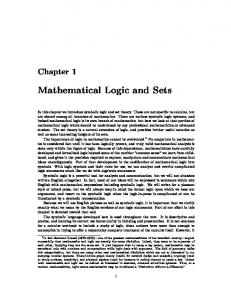


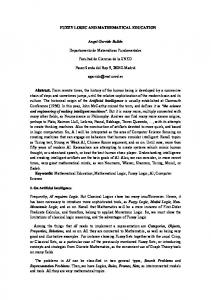

![[PDF] Discrete Structures, Logic, And Computability Full ... - Google Sites](https://m.moam.info/img/260x300/pdf-discrete-structures-logic-and-computability-fu_6477aa89097c47a9708bf779.jpg)

![([PDF]) Discrete Structures, Logic, And Computability ... - Google Sites](https://m.moam.info/img/260x300/pdf-discrete-structures-logic-and-computability-go_6477f466097c474b228ca710.jpg)
![[PDF] Discrete Structures, Logic, And Computability ... - Google Sites](https://m.moam.info/img/260x300/pdf-discrete-structures-logic-and-computability-go_6477c19e097c4786708c1039.jpg)


