([Pol07]), although the density and location of such cross-links remains to be ... simplified by carrying out the limit of instantaneous cross-link and adhesion ...
HOW DO CELLS MOVE? MATHEMATICAL MODELLING OF CYTOSKELETON DYNAMICS AND CELL MIGRATION. ¨ DIETMAR OLZ AND CHRISTIAN SCHMEISER Abstract. We present a novel approach to the modelling of the lamellipodial Actin-cytoskeleton meshwork. The model is derived starting from the microscopic description of mechanical properties of filaments and cross-links and also of the life-cycle of cross-linker molecules. The result is a mulitphase evolution model for lamellipodia with arbitrary shape which allows us to relate computationally the structure and dynamics of the Actin network to the traction forces and shape changes that constitute the amoeboid movement of cells.
1. Introduction The description of cell migration by the action of a lamellipodium given in [OSS08] is reproduced here for completeness: Cells migrate by protruding at the front and retracting at the rear. Protrusion occurs in thin membrane bound cytoplasmic sheets, 0.2-0.3 µm thick and several microns long, termed lamellipodia ([SSVR02]). The major structural components of lamellipodia are actin filaments, which are organised in a more or less two-dimensional diagonal array with the fast growing, plus ends of the actin filaments directed forwards, abutting the membrane ([SIC78]). Protrusion is effected by actin polymerisation, whereby actin monomers are inserted at the plus ends of the filaments at the membrane interface and removed at the minus ends, throughout and at the base of the lamellipodium, in a treadmilling regime ([PLCC01]). Stabilisation of the actin meshwork is achieved by the cross-linking of the filaments by actin-associated proteins, such as filamin ([NOH+ 07]) as well as protein complexes, such as the Arp2/3 complex ([Pol07]), although the density and location of such cross-links remains to be established. Since actin polymerisation is involved in diverse motile processes aside from cell motility, including endocytosis and the propulsion of pathogens that invade cytoplasm ([CP07]), the question of how actin filaments are able to push against a membrane has spawned the development of various models ([Mog06]). Modelling efforts go back to 1996 and fall into two groups. The first group includes continuum models for the mechanical behaviour of cytoplasm: a two phase formulation for cytosol and the actin network [AD99]; a one dimensional viscoelastic model [GO04]; a one dimensional model for the actin distribution [MMB]; and a two dimensional elastic continuum model [RJM05]. The second group makes presumptions about the microscopic organisation of the actin network. The Brownian ratchet model for the polymerisation process introduced by Mogilner and Oster [MO96] considers actin cross-linking proteins as stabilizers of the lamellipodium meshwork, allowing enough flexibility for actin filaments to bend away from the membrane to accept actin monomers. Other models are based on the current idea ([Pol07]), that the actin filaments in lamellipodia form a branched network with the Arp2/3 complex at the branch points 1991 Mathematics Subject Classification. Primary: 92C10 Secondary: 92C17, 92C37, 74L15, 74A25, fehlt noch was. Key words and phrases. Modelling, Cell Movement. 1
2
¨ DIETMAR OLZ AND CHRISTIAN SCHMEISER
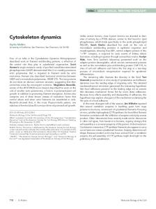
[MB01, STB07, L+ 06]. A related model considers the lamellipodia as constructed from short filaments that take one of six orientations [MJD+ 06]. Recent studies have indicated that filaments in lamellipodia are not organised in branched arrays ([KAV+ 08]). Rather, the pseudo-two-dimensional actin network contains unbranched filaments whereby the filament density decreases from the front to the rear of the lamellipodium, indicative of a graded distribution of filament lengths. According to this structural information, we present a quasi-stationary modelling approach for the simulation of the turnover of the lamellipodium surrounding a cell on a flat substrate. This corresponds to in vitro situations such as cytoplasmic fragments of keratocytes [VSB98]. Our approach differs from previous ones in that we describe the lamellipodium in terms of a continuous distribution of filaments of graded length and their linkages. In this work the models from [OSS08] and [OS08a] are generalized from rotationally symmetric to arbitrary geometries. Otherwise, the assumptions on the mechanics of the network are the same: there is an elastic resistance against bending of actin filaments, against stretching and twisting of cross-links between the filaments, against polymerisation of the barbed ends by the membrane, and against the stretching of trans-membrane linkages (called adhesions) between filaments and the substrate. In the following section the basic model is derived with a detailed probabilistic account of the life cycle of cross-links and adhesions. In Section 3 the model is simplified by carrying out the limit of instantaneous cross-link and adhesion turn-over. A picture from a time dependent simulation is reproduced from [OS08b], where numerical methods for simulations with the limiting model are presented. Finally, the connection to the results from [OSS08] and [OS08a] is established in Section 4 by showing that the general model possesses rotationally symmetric solutions. An analysis of the stability of a trivial steady state illustrates simulation results presented in [OSS08]. 2. Modelling A central feature of the model is an age-structured production/decay of cross-links and adhesions, consistent with dynamic association/dissociation of linkage molecules with the actin network. In order to obtain a feasible mathematical description we will adopt a homogenisation limit, based on the assumption that the density of filaments within the lamellipodium is very high. We let the number of filaments tend to infinity in order to obtain a model based on continuous quantities instead of discrete ones. The assumptions made are as follows: A1: The lamellipodium is two dimensional and has the topology of a ring, i.e. it lies between two closed curves. A2: All actin filaments belong two one of two families, called clockwise and anti-clockwise. Filaments of the same family do not cross each other. Crossings of clockwise with anti-clockwise filaments are transversal. All barbed ends touch the leading edge of the lamellipodium, i.e. the outer curve of the previous assumption. Filaments are inextensible. A3: Filaments polymerise at the barbed ends with given polymerisation speed. Depolymerisation at the pointed ends is a stochastic process with prescribed distribution. As a consequence of A1 and A2 the lamellipodium has the organisation depicted in Figure 1. There are two families of locally parallel filaments. Looking from the centre of the lamellipodium ring, the filaments in the first group bear to the right and the second group to the left (relative to each other); referred to as clockwise and anti-clockwise filaments, respectively. We assume the presence of n+ clockwise filament with indices i = 0, ..., n+ − 1 and n− anticlockwise filament with indices j = 0, ..., n− − 1. An arc length parametrisation of the clockwise
MATHEMATICAL MODELLING OF CYTOSKELETON DYNAMICS
3
Figure 1. Constituent elements of the model. + 2 filaments at time t is given by {Fi+ (t, s) : −L+ i (t) ≤ s ≤ 0} ⊂ R , where s = −Li (t) corresponds to the pointed end and s = 0 to the barbed end. Analogously we represent the anti-clockwise + − 2 filaments at time t by {Fj− (t, s) : −L− j (t) ≤ s ≤ 0} ⊂ R such that |∂s Fi | ≡ |∂s Fj | ≡ 1. − The lengths L+ i (t) and Lj (t) of the filaments are random variables whose distributions are considered as given by + P (−L+ i (t) ≤ s) = ηi (t, s) ,
− P (−L− j (t) ≤ s) = ηj (t, s) .
The arclength s is a geometric parameter. Because of the polymerisation at the barbed ends, polymerised actin molecules travel along the filament towards the pointed ends with the polymerisation speed denoted by vi+ (t) and vj− (t) respectively. Because of this and because of the inextensibility assumption inR A2, Lagrange variables along the filaments are given by Rt t σi+ = s + 0 vi+ (t˜)dt˜ and σj− = s + 0 vj− (t˜)dt˜. In other words, the path of the actin molecule � � Rt with label σi+ on the clockwise filament Fi+ is given by Fi+ t, σi+ − 0 vi+ (t˜)dt˜ . The fact that only depolymerisation happens at the pointed ends is reflected by the assumption that Z t Z t + + ˜ ˜ − −Li (t) + vi (t)dt and − Lj (t) + vj− (t˜)dt˜ 0
0
are increasing functions of time. As a consequence, the distribution functions ηi+ and ηj− are decreasing with respect to time when written in terms of the Lagrangian variables. In other words, ∂t ηi+ − vi+ ∂s ηi+ ≤ 0 and ∂t ηj− − vj− ∂s ηj− ≤ 0. The next step is to describe the kinematics of cross-links, and we start with the modelling assumptions: A4: A cross-link is a connection between a material point on a clockwise and a material point on an anti-clockwise filament. Cross-links can be created spontaneously at the crossing between two filaments and they can also break. Creation and breaking are stochastic processes. There exists at most one cross-link for any pair of filaments at any time.
¨ DIETMAR OLZ AND CHRISTIAN SCHMEISER
4
For the creation of cross-links, we need the information about filament crossings. We assume that each clockwise filament crosses each anti-clockwise filament at most once. At time t, the crossings are described by a set of index pairs: − + + − − C(t) := {(i, j) : ∃ s+ i,j (t), si,j (t) such that Fi (t, si,j (t)) = Fj (t, si,j (t))} .
If a cross-link between the filaments with indices i and j is created at time t∗ , then this happens at the crossing point. Once established, however, the two binding sites will travel with the material along the two filaments. Thus, at a later time t = t∗ + a, the binding sites will be located at Z t + + + + Fi (t, sa,i,j (t)) , sa,i,j (t) := si,j (t − a) − v + (t˜)dt˜, Fj− (t, s− a,i,j (t)) ,
− s− a,i,j (t) := si,j (t − a) −
t−a t
Z
v − (t˜)dt˜,
t−a
until the cross-link eventually breaks. We call a the age of the cross-link. Below we shall assume a resistance of cross-links against stretching and twisting. This means there are elastic forces related to the stretching − − Si,j (t, a) := Fi+ (t, s+ a,i,j (t)) − Fj (t, sa,i,j (t)) ,
and to the twisting Ti,j (t, a) := ϕi,j (t, a) − ϕ0 , where
h i − − ϕi,j (t, a) := arccos ∂s Fi+ (t, s+ (t)) · ∂ F (t, s (t)) s a,i,j j a,i,j
is the angle between the directions of the filaments at the binding sites, and ϕ0 is an equilibrium angle determined by the properties of the cross-linking molecule. We allow also obtuse angles 0 ≤ ϕ, ϕ0 ≤ π allowing for cross-linkers sensitive to the orientation of actin filaments. The probability distribution for the existence of a cross-link with respect to age will be denoted by ri,j (t, a), where Z ∞ (2.1) ri,j (t, a) da ≤ 1 0
is the probability that a cross-link between the the ith clockwise filament and the jth anticlockwise filament exists at time t. We postulate the following model for the evolution of the distribution: � � Z ∞ (2.2) ∂t ri,j + ∂a ri,j = −ζ(Si,j , Ti,j )ri,j , ri,j (t, 0) = β(Ti,j (t, 0)) 1 − ri,j (t, a) da , 0
This model has the standard form of age-structured population models (see, e.g., [Per07]). The differential equation describes ageing and breaking of cross-links, the boundary condition at a = 0 describes their creation. The dependence of the breaking rate on stretching and twisting reflects that a cross-link might be broken by being loaded too much. The twisting dependence of the creation rate β could eliminate the possibility for a cross-link to be established, if the angle between the filaments is too far from the equilibrium angle. Integration of the differential equation with respect to a shows that the second factor in the creation rate guarantees (2.1), i.e., the fact that there is at most one cross-link. Just as for the pointed-end (de)polymerisation process, all we need to know about the processes of creation and breaking of cross-links is the distribution ri,j .
MATHEMATICAL MODELLING OF CYTOSKELETON DYNAMICS
5
Figure 2. The domain of the differential equation in (2.2) is determined by the requirement that both binding sites (on the ith clockwise filament and on the jth anti-clockwise filament) have not + − − been depolymerised yet: s+ a,i,j (t) ≥ −Li (t), sa,i,j (t) ≥ −Lj (t). The next modelling step is the passage to a continuum description by letting the total numbers of filaments n+ and n− tend to infinity. In the limit, the discrete indices αi+ = π(2i/n+ − 1), i = 0, . . . , n+ − 1 and αj− = π(2j/n− − 1), j = 0, . . . , n− − 1 are replaced by a continuous parameter α ∈ [−π, π). Then we interpret the discrete filament positions Fi+ (t, s) and Fj− (t, s) as approximations for the values F + (t, αi , s) and, respectively, F − (t, αj , s) of continuous functions F ± : [0, ∞) × B → R2 ,
with B := [−π, π) × [−L, 0] ,
where L is a maximal length of filaments. Note that we assume periodicity of B in the sense that all functions of α are 2π-periodic. The fact that filaments of the same family do not cross, implies that F ± (t, ·) has to be one-to-one. The shape of the lamellipodium at time t is given by Ω(t) = F + (t, B) ∪ F − (t, B). According to Assumption 1, its boundary consists of an inner and an outer curve: ∂Ω(t) = ∂Ωin (t) ∪ ∂Ωout (t). The fact that, by Assumption 2, all barbed ends touch the leading edge, takes the mathematical form ∂Ωout (t) = {F ± (t, α, 0) : −π ≤ α < π}. Continuous versions of the length distributions ηi+ and ηj− are given by η ± : [0, ∞) × B → [0, 1] , now getting the deterministic interpretation as the expected fraction of filaments in each index element dα, whose length at time t is bigger than −s. They are nondecreasing functions of s satisfying η ± (t, α, 0) = 1.
6
¨ DIETMAR OLZ AND CHRISTIAN SCHMEISER
Crossings of filaments can only occur in Ωc (t) = F + (t, B) ∩ F − (t, B) ⊂ Ω(t). Similar to C(t), we construct a set of index pairs by � C(t) = (α+ , α− ) ∈ [0, 2π)2 : ∃ s± (t, α+ , α− ) such that F + (t, α+ , s+ (t, α+ , α− )) = F − (t, α− , s− (t, α+ , α− )) which corresponds to the discrete set C(t) in the sense that (αi , αj ) ∈ C(t) if (i, j) ∈ C(t). Consistent with the assumption that two given filaments cross at most once, we assume that for each pair (α+ , α− ) ∈ C(t) there is only one s± (t, α+ , α− ). Defining B ± (t) := {(α± , s± (t, α+ , α− )) : (α+ , α− ) ∈ C(t)} ⊂ B , the maps (α+ , α− ) 7→ (α± , s± (t, α+ , α− )) from C(t) to B ± (t) are invertible. Combining one of them with the other’s inverse gives an invertible map (α+ , s+ ) 7→ (α− (t, α+ , s+ ), s− (t, α+ , s+ )) from B + (t) to B − (t). We complete the description of the geometry of crossings by defining the angle between crossing filaments: � � ϕ(t, α+ , α− ) = arccos ∂s F + (t, α+ , s+ (t, α+ , α− )) · ∂s F − (t, α− , s− (t, α+ , α− )) . We introduce the polymerisation rates v ± (t, α) such that vi+ approximates v + (t, αi ) and vj− approximates v − (t, αj ) and abbreviate the s-values at time t of cross-links with age a by Z t + − + + − s+ (t, α , α ) := s (t − a, α , α ) − v + (t˜, α+ )dt˜, a + − − + − s− a (t, α , α ) := s (t − a, α , α ) −
t−a t
Z
v − (t˜, α− )dt˜.
t−a
The age-depedent probability distribution of cross-links can be understood as an expected crosslink density ρ(t, α+ , α− , a) with (α+ , α− ) ∈ C(t − a). This condition means that for a cross-link of age a connecting the filaments with labels α+ and α− to exist at time t, the filaments must have crossed at time t − a. From (2.2) the transport equation for the cross-link density becomes ∂t ρ + ∂a ρ = −ζ(S, T )ρ .
(2.3)
Boundary conditions are required at a = 0, describing the creation of new cross-links, and for (α+ , α− ) ∈ ∂C(t − a)+ , with ∂C(t − a)+ denoting the part of the boundary of C(t − a), where the filaments with labels α+ and α− start to have a crossing. In other words, the time direction points into the domain of ρ at these points. The boundary datum there has to be zero, since there are no pre-existing cross-links. So the boundary conditions are � � Z ∞ (2.4) ρ(a = 0) = β(T0 ) 1 − ρ da , ρ(t, α+ , α− , a) = 0 for (α+ , α− ) ∈ ∂C(t − a)+ , 0
with T0 = T (a = 0). Note that the upper bound in the integration should actually be t − t0 (α+ , α− ) with (α+ , α− ) ∈ ∂C(t0 )+ , but for simplicity we consider the definition of ρ as continued by zero to arbitrary values of a > 0. The stretching and twisting terms are now given by (2.5) (2.6)
+ − − − − + − S(t, α+ , α− , a) = F + (t, α+ , s+ a (t, α , α )) − F (t, α , sa (t, α , α )) , T (t, α+ , α− , a) = ϕa (t, α+ , α− , a) − ϕ0 ,
with � � + − − − − + − ϕa (t, α+ , α− ) = arccos ∂s F + (t, α+ , s+ a (t, α , α )) · ∂s F (t, α , sa (t, α , α )) .
MATHEMATICAL MODELLING OF CYTOSKELETON DYNAMICS
7
The boundedness property (2.1) of the microscopic cross-link density determined by (2.2) carries over to the modified model (2.3), (2.4). The accumulated distribution Z ∞ + − ρ(t, α+ , α− , a) da ρ¯(t, α , α ) = 0
satisfies the equation Z
∞
ζρ da + β (1 − ρ¯) ,
∂t ρ¯ = − 0
preserving the property 0 ≤ ρ¯(t, α+ , α− ) ≤ 1. Taking into account the length distribution of the filaments, we arrive at the effective crosslink density + − − − − + − ρeff (t, α+ , α− , a) = ρ(t, α+ , α− , a)η + (t, α+ , s+ a (t, α , α ))η (t, α , sa (t, α , α )) ,
where each of the two filaments involved in a cross-link contributes a factor η ± . Note that ρeff satisfies � � ∂t η + − v + ∂s η + ∂t η − − v − ∂s η − ∂t ρeff + ∂a ρeff = −ρeff ζ(S, T ) − , − η+ η− hence the same type of transport equation as ρ but with a modified decay rate, which takes into account the loss of cross-links due to depolymerisation of the pointed ends. Note that, just as in the microscopic model, the fact that only depolymerization happens at the point ends is described by the inequality ∂t η ± − v ± ∂s η ± ≤ 0.
Figure 3. Detailed view at cross-links Now we turn to the dynamics of adhesion molecules: A5: An adhesion is a connection between a material point on a filament and a point on the substrate via a transmembrane linkage. Adhesions can be created spontaneously and they can also break. Creation and breaking are stochastic processes. The number of adhesions per filament length is restricted.
¨ DIETMAR OLZ AND CHRISTIAN SCHMEISER
8
The densities ρ± adh (t, α, s, a) of adhesions on clockwise and anti-clockwise filaments, respectively, satisfy the differential equations ± ± ± ± adh ∂t ρ± (Sadh )ρ± adh + ∂a ρadh − v ∂s ρadh = −ζ adh ,
(2.7)
with the boundary conditions (2.8)
ρ± adh (a
= 0) = β
adh
� Z adh ρ¯max − 0
∞
ρ± adh da
� ,
ρ± adh (s = 0) = 0 ,
adh where ρ¯adh max is the maximal density of cross-links along the filament and the breaking rate ζ depends on the stretching of the adhesions: � � Z t ± ± ˜ ± ± t − a, α, s + v (t, α)dt˜ . Sadh (t, α, s, a) = F (t, α, s) − F t−a
Like for the cross-link density, the second boundary condition means that there are no preexisting adhesions on newly polymerized parts of the filaments. It remains to formulate assumptions determining the position of the filaments: A6: The position of the filaments is determined by a quasistationary balance of elastic forces resulting from bending the filaments, stretching and twisting the cross-links, stretching the adhesions, and stretching the cell membrane around the leading edge. The quasistationarity assumption means that elastic oscillations are neglected, since the filament network is damped by viscous forces in the cytosol. Thus, the dynamics of the network results only from (de)polymerisation and from the creation and breaking of cross-links and adhesions. Mathematically, the Assumption A6 will be formulated by assuming that the filament positions minimize a potential energy functional containing contributions from the above mentioned elastic effects. We require the functions F + (t, ·, ·) and F − (t, ·, ·) to minimize the functional (2.9)
− + (t)[G− ] + Uscl+tcl (t)[G+ , G− ] (t)[G+ ] + Ubending U (t)[G+ , G− ] := Ubending + − +Umembrane [G± ] + Uadh (t)[G+ ] + Uadh (t)[G− ]
The energy contribution from bending the filaments is the Kirchhoff bending energy from standard linearized beam theory: Z κB ± ± Ubending (t)[G ] := |∂ 2 G± |2 η ± d(α, s) 2 B s where κB is the bending stiffness of one filament. The stretching and twisting energy of the crosslinks is modelled by � S � Z ∞Z κ κT 2 + − 2 Uscl+tcl (t)[G , G ] := |S| + T ρeff d(α+ , α− ) da 2 2 0 C(t−a) with the quantities S and T from (2.5) and (2.6) applied to G+ and G− respectively. The constants κS and κT are Hooke constants describing the stretching and, respectively, torsional stiffnesses of the cross-link molecules. Furthermore the energies associated to the stretching of integrins on clockwise and anticlockwise filaments, respectively, read (2.10) � � 2 Z Z ∞ Z t ± κF ± ± ± ˜ G − F ± t − a, α± , s + ˜ ρ± η ± da d(α, s) . Uadh (t)[G ] := v ( t , α) d t adh 2 B 0 t−a
MATHEMATICAL MODELLING OF CYTOSKELETON DYNAMICS
9
Note that the evaluation of the adhesion energy and of the cross-link stretching and twisting energy at time t requires information on previous filament positions. Because of the treadmilling of filaments, the lifetime of monomers in a filament and, thus, of binding sites of cross-links and adhesion molecules is finite. The densities ρeff and ρ± adh have compact supports in the age direction and the above integrals with respect to a can be restricted to these supports. It is obvious that past filament positions enter in the computation of the adhesion energy. However, this is also the case for the energy in cross-links, where past filament positions enter in the computation of s± a. It remains to model the action of the cell membrane on the leading edge of the network: A7: The cell membrane simulates a rubber band stretched around the barbed ends of the filaments. This leads to a model of the form � + + �2 C [G ] + C − [G− ] ± M Umembrane [G ] := κ − C0 , 2 + with the circumference of the lamellipodium C + [G+ ] = C − [G− ], given by either one of the two equivalent formulations Z π ± ± C [G ] := |∂α G± (t, α, 0)| dα . −π
The arithmetic mean is used in the energy for symmetry reasons. This models resistance against stretching the membrane above the equilibrium circumference C0 . The positions of the filaments at time t is now determined by minimizing the energy: (2.11)
U (t)[F + (t, ·, ·), F − (t, ·, ·)] = min U (t)[G+ , G− ] ,
under the constraint of inextensibility (2.12)
|∂s G+ | = |∂s G− | = 1 ,
and under the constraint that all barbed ends touch the leading edge: (2.13)
{G+ (t, α, 0) : −π ≤ α < π} = {G− (t, α, 0) : −π ≤ α < π} .
The formulation of a well posed problem still requires a start-up procedure. It first involves a decision about the maximal age A of all cross-links and adhesions which are present at time t = 0. In other words, initial data ρ(0, α+ , α− , a) and ρ± adh (0, α, s, a) have to be prescribed, which vanish for a > A. In order to be able to compute the binding sites of all the initial cross-links and adhesions, the positions F ± (t, α, s) of the filaments for −A ≤ t ≤ 0 have to be given. 3. The limit of instantaneous cross link and adhesion turnover For two reasons, numerical simulations with the model presented in the previous section are very costly. On the one hand, the densities of cross-links and adhesions are functions of three variables ((α+ , α− , a) and (α, s, a), respectively). On the other hand, the problem for the deformation of the filaments is a delay problem, such that the history of the filament dynamics has to be stored up to the maximal age of cross-links and adhesions. Therefore a simplification will be carried out below, which can also be motivated by the fact that in the model macroscopic and microscopic scales are still mixed. The typical length and bending radius of a filament will in general be large compared to the size of a cross-linking or adhesion molecule, even when the latter is stretched, as assumed in our model. This also makes it plausible that the life time of such a connection is short compared to the typical time scale for the dynamics of the network. We shall make this assumption, although it is not true for all
10
¨ DIETMAR OLZ AND CHRISTIAN SCHMEISER
applications. It means for example that we exclude the build-up of large adhesion complexes from our considerations. Asymptotic methods will be used to derive an approximative problem, where the cross-link and adhesion densities can be computed explicitly. Also the delays disappear, and the problem becomes local in time at the expense of time derivatives appearing in the equations for the filament displacements. A physical interpretation of the approximation is that the rapid turnover of cross-links and adhesions can be described as effective friction. A nondimensionalisation is carried out, where the typical filament length L is used as reference length for scaling s, F ± , S± , Sadh , and C0 . With v0 being the reference speed for the polimerisation speed v± , the reference time L/v0 for scaling t is the typical time an actin molecule spends in a filament between polymerization at the barbed end and depolymerization at the pointed end. The birth and death rates of cross-links and adhesions β, ζ, β adh , and ζ adh will be assumed to be of the same order of magnitude with a typical value 1/¯ a used for nondimensionalisation, where a ¯ can be interpreted as typical life time of cross links and adhesions. Our main scaling assumption is that the dimensionless parameter ε :=
a ¯v0 , L
is small. The reference values for the densities of cross links and of adhesions are 1/(¯ aL) and, respectively, ρ¯adh /¯ a . Finally, energy (U and all its contributions) is scaled with the reference max value κB L, and the reference values for κS , κT , κA , and κM , are κB /(εL), κB L, κB /(ε¯ ρadh max L), B and κ /L, respectively. For notational simplicity, the same symbols will be used for the nondimensionalised quantities as for their dimensional counterparts. The filament displacement F ± (t, ·, ·) is determined as a minimizer (with the side conditions (2.12) and (2.13)) of the sum of the scaled energy contributions �2 � + + − − [G ] Umembrane [G± ] := κM C [G ]+C − C , 0 2 + R ± 1 2 ± 2 ± ± Ubending (t)[G ] = 2 B |∂s G | η d(α, s) , S R∞R (3.1) Uscl (t)[G+ , G− ] = κ2ε 0 C(t−εa) |S|2 ρeff d(α+ , α− ) da , T R∞R Utcl (t)[G+ , G− ] = κ2 0 C(t−εa) T 2 ρeff d(α+ , α− ) da , F R∞R 2 ± ± Uadh (t)[G± ] = κ2ε 0 B |G± − F ±∗ | ρ± adh η d(α, s) da , with (3.2)
+ − − − − + − S = G+ (t, α+ , s+ εa (t, α , α )) − G (t, α , sεa (t, α , α )) , + − T = ϕεa (t, α , α ) − ϕ0 .
and (3.3)
� Z F ±∗ := F ± t − εa, α± , s +
t
� v ± (t˜, α) dt˜ .
t−εa
The problems for the cross link density and for the adhesion density become
(3.4)
ε∂t ρ + ∂a ρ = −ζ(S, T )ρ , � R∞ ρ(a = 0) = β(T0 ) 1 − 0 ρ da , ρ(t, α+ , α− , a) = 0 for (α+ , α− ) ∈ ∂C(t − εa)+ , ρ(t = 0) = ρI .
MATHEMATICAL MODELLING OF CYTOSKELETON DYNAMICS
11
with T0 = arccos [∂s F + (t, α+ , s+ ) · ∂s F − (t, α− , s− )] − ϕ0 and, respectively, ± ± ± adh εDt± ρ± adh + ∂a ρadh = −ζ R (Sadh )ρadh �, ∞ ± ± adh ρadh (a = 0) = β 1 − 0 ρadh da , (3.5) ρ± adh (s = 0) = 0 , ± ρ± adh (t = 0) = ρadh,I . Rt ± with Sadh (t, α± , s, a) = F ± (t, α± , s) − F ± (t − εa, α± , s + ε t−a v ± (t˜) dt˜). For notational convenience, the material derivative
Dt± := ∂t − v ± ∂s
(3.6)
is used here and in the following. The reason for the scaling assumption that the stiffnesses of the adhesions and of the crosslinks against stretching are O(ε−1 ) relative to the other stiffnesses is a priori not obvious. Actually, when replacing G± (α± , s) by the minimizer F ± (t, α± , s), the energies Uscl (t)[F + , F − ] and Uadh (t)[F ± ] are formally O(ε). It will be shown below that in the limit ε → 0 they still contribute to the minimization conditons. The above mentioned approximation is derived by passing to the limit ε → 0. We start with (3.5). The formal limiting equations � � Z ∞ ± ± ± ± adh adh ρadh da , ∂a ρadh = −ζ (0)ρadh , ρadh (a = 0) = β 1− 0
have the solution β adh ζ adh (0) −ζ adh (0)a e . β adh + ζ adh (0) This is a singular limit, since the small parameter ε multiplies the material derivative. As a consequence, the conditions at s = 0 and at t = 0 cannot be satisfied by the limiting (outer, in the language of singular perturbation theory) solution. We ignore eventual boundary and initial layers (i.e., thin regions close s = 0 and t = 0 with strong variation of the solution). Analogously we deal with (3.4). The main difference is that the limiting equations � � Z ∞ ∂a ρ = −ζ(0, T0 )ρ , ρ(a = 0) = β(T0 ) 1 − ρ da , ± ρ± adh (t, α , s, a) =
0
and therefore also the limiting solution ρ=
β(T0 )ζ(0, T0 ) −ζ(0,T0 )a e β(T0 ) + ζ(0, T0 )
depend on the displacement of the filaments via T0 . As announced above, the dependence is local in time. If the limit ε → 0 is carried out formally in (3.1), the contributions from the adhesions and from stretching the cross links disappear. In order to reveal their influence, the solution of the variational problem needs to be discussed. The displacement F ± (t, ·, ·) at time t has to satisfy the variational equation δU [F + , F − ](δF + , δF − ) = 0 for all admissible variations (δF + , δF − ), where δU is the variation of the total energy, i.e., the sum of all terms in (3.1). Admissibility conditions for the variations are a consequence of the constraints |∂s F ± | ≡ 1 and {F + (t, α, 0) : −π ≤ α < π} = {F − (t, α, 0) : −π ≤ α < π}. The
¨ DIETMAR OLZ AND CHRISTIAN SCHMEISER
12
derivation of a strong formulation of the variational equations will be facilitated by a Lagrange multiplier approach, where we employ the additional functionals Z 1 ± ± Uext [G ] = λ± (α, s)(|∂s G± (α, s)|2 − 1)η ± d(α, s) , 2 B describing extension of filaments, and Z π + − Uedge [G , G ] = λedge (α+ )(G+ (t, α+ , 0) − G− (t, α ˆ (t, α+ ), 0)) · ν(t, α+ )dα+ , −π
describing the deviation between the outer edges of both filament families. Here α ˆ (t, α+ ) is + + − + + chosen such that G (t, α , 0) − G (t, α ˆ (t, α ), 0) is parallel to ν(t, α ), the outward unit normal vector along the barbed ends of the clockwise filaments, which can be computed from ∂α G+ (t, α+ , 0). In the following the variations of the energy contributions and their limits as ε → 0 are computed individually. (1) The variation of the stretching energy of the membrane reads Z π � ∂α F ± (s = 0) ± ± M ± δUmembrane [F ]δF = κ C − C0 + · ∂α δF ± (s = 0) dα , ± (s = 0)| |∂ F α −π with the same expression in the limit ε → 0. (2) For the variation of the bending energy of the filaments we obtain Z ± ± ± δUbending [F ]δF = ∂s2 F ± · ∂s2 δF ± η ± d(α, s) , B
again with the same expression for ε → 0. (3) The variation of the energy contribution by stretching the cross-links can now be written as Z Z κS ∞ + − + − ± SδF ± (t, α± , s± δUscl (t)[F , F ]δF = ± εa ) ρeff d(α , α ) da . ε 0 C(t−εa) We may write (3.2) as + + + + − S =F + (t, α+ , s+ εa ) − F (t − εa, α , s (t − εa, α , α )) − + − + − −(F − (t, α− , s− εa ) − F (t − εa, α , s (t − εa, α , α ))) .
(3.7)
This implies S = εa(Dt F + − Dt F − ) + O(ε2 ), and therefore passing to the limit ε → 0 gives Z + − ± δUscl (t)[F , F ]δF = ± µS (T0 )(Dt F + − Dt F − )δF ± η + η − d(α+ , α− ) , C(t)
with (3.8)
S
S
Z
µ (T0 ) = κ
∞
aρ da = 0
κS β(T0 ) . ζ(0, T0 )(β(T0 ) + ζ(0, T0 ))
(4) Before we compute the variation of the twisting energy, we observe that our formula for the angle between filaments is only valid if the constraint |∂s F ± | = 1 holds. Since, in the Lagrange multiplier approach, also variations are allowed which violate this condition, we reformulate the definition of the angle as cos ϕεa =
∂s F + ∂s F − + (s = s ) · (s = s− εa εa ) . |∂s F + | |∂s F − |
MATHEMATICAL MODELLING OF CYTOSKELETON DYNAMICS
� � x With T = ϕεa − ϕ0 and δ |x| δT [F + , F − ]δF ± = −
|x|=1
13
= (x⊥ · δx)x⊥ ((x1 , x2 )⊥ = (−x2 , x1 )) we obtain
(∂s F ±⊥ · ∂s F ∓ )(∂s F ±⊥ · ∂s δF ± ) = ∓∂s F ±⊥ · ∂s δF ± , sin ϕεa
where ∂s F ± and ∂s δF ± are evalutated at (t, α± , s± εa ). The sign in the last term is due to the fact that the superscript + indicates the family of clockwise filaments. It then holds that Z ∞Z + − ± T T (∂s F ±⊥ · ∂s δF ± )ρeff d(α+ , α− ) da , δUtcl (t)[F , F ]δF = ∓κ 0
C(t−εa)
and therefore, as ε → 0, we conclude Z + − ± δUtcl (t)[F , F ]δF = ∓ µT (T0 )T0 (∂s F ±⊥ · ∂s δF ± )η + η − d(α+ , α− ) , C(t)
where now ∂s
F±
are evalutated at (t, α± , s± (t, α+ , α− )) and Z ∞ κT β(T0 ) T T ρ da = µ (T0 ) = κ . β(T0 ) + ζ(0, T0 ) 0
and ∂s
(3.9)
δF ±
(5) The variation of the stretching energy of the adhesions is straightforward and reads Z Z κA ∞ ± ± ± ± δUadh [F ]δF = (F ± − F ±∗ ) · δF ± ρ± adh η d(α, s) da . ε 0 B In the limit ε → 0, a material derivative occurs similarly to the stretching of the cross links: Z ± Dt± F ± · δF ± η ± d(α, s) , (3.10) δUadh [F ± ]δF ± = µA B
with A
(3.11)
A
Z
∞
µ =κ
aρadh da =
0
κA β adh . ζ adh (0)(β adh + ζ adh (0))
(6) In the two Lagrangian terms, we do not include the contributions form the variation of the Lagrange multipliers. For the inextensibility term we obtain Z ± ± ± δUext [F ]δF = λ± ∂s F ± · ∂s δF ± η ± d(α, s) . B
(7) The term which guarantees that all pointed ends touch the leading edge gives Z π + − ± ± δUedge [F , F ]δF = ± λ± edge ν · δF (s = 0) dα , −π
where
λ+ edge
= λedge (α) and
λ− edge
= λedge (α+ (t, α, 0)).
Collecting the terms computed under (1)–(7) leads to the variational equation � Z π� � ∂α F ± ± ± ± (3.12) · ∂ δF ± λ ν · δF dα κM C ± − C 0 + α edge |∂α F ± | −π s=0 Z � � ± µS (T0 )(Dt F + − Dt F − )δF ± − µT (T0 )T0 ∂s F ±⊥ · ∂s δF ± η + η − d(α+ , α− ) C(t) Z � + ∂s2 F ± · ∂s2 δF ± + µA Dt± F ± · δF ± + λ± ∂s F ± · ∂s δF ± η ± d(α, s) = 0 , B
¨ DIETMAR OLZ AND CHRISTIAN SCHMEISER
14
where now there is no restriction on the variations δF + and δF − . The first integral corresponds to the leading edge and will contribute boundary conditions to a strong formulation of the problem. From the second and third integrals the Euler-Lagrange equations will be derived. For that purpose the integration domains have to mapped to each other. Noting that in the second integral F ± and δF ± and their derivatives are evaluated at (t, α± , s± ), we employ the transformations (α+ , α− ) 7→ (α, s) = (α± , s± (t, α+ , α− )). We incorporate the corresponding Jacobians and the fact that these terms only contribute in B ± (t) into the macroscopic stiffness parameters for the cross-links: ∓ ∓ ( ( ∂α S ± T µ ∂s± in B (t) , µ ∂α in B ± (t) , ∂s± µS± = µT± = 0 in B \ B ± (t) , 0 in B \ B ± (t) , where the interpretation of the additional factor is the number of crossings per unit length. The Euler-Lagrange equations are given by (3.13) ∂s2 (η ± ∂s2 F ± ) − ∂s (η ± λ± ∂s F ± ) + η ± µA Dt± F ± � � � � ±∂s η + η − µT± (ϕ − ϕ0 )(ϕ − ϕ0 )∂s F ±⊥ ± η + η − µS± (ϕ − ϕ0 ) Dt+ F + − Dt− F − = 0 . The terms in the first row correspond to standard linear models for the deformation of beams. The first term corresponds to bending, the second to stretching (just the right amount such that |∂s F ± | = 1 holds), and the third to friction caused by adhesion to the substrate. All these terms are evaluated at (t, α, s) and, obviously none of them generates any coupling in α, i.e., between different filaments. The terms in the second line describe the effects of cross-linking. Note that, in the equation for F + , the derivatives of F − have to be evaluated at (t, α− (t, α, s), s− (t, α, s)) and vice versa, employing the mapping between B + (t) and B − (t). The last term shows that the macroscopic effect of the resistance against stretching of cross-links is friction caused by the relative motion of the two filament families. The solution of the Euler-Lagrange equations (3.13) have to satisfy the boundary conditions −∂s (η ± ∂s2 F ± ) + η ± λ± ∂s F ± ∓ η + η − µT± (ϕ − ϕ0 )∂s F ±⊥ = 0 , ∂s (η ± ∂s2 F ± )
±
− λ ∂s F
±
±
µT± (ϕ
M = ±λ± edge ν − κ
(3.14) η ± ∂s2 F ± = 0 ,
for s = −L ,
±⊥
− ϕ0 )∂s F � � � ∂α F ± ± , C − C0 + ∂ α |∂α F ± |
for s = 0 ,
for s = −L, 0 .
The Lagrange parameters λ± and λedge have to be determined such that the constraints are satisfied: (3.15) |∂s F + | = |∂s F − | = 1 ,
{F + (t, α, 0) : −π ≤ α < π} = {F − (t, α, 0) : −π ≤ α < π} .
Figure 4 shows one frame of a time dependent simulation carried out in [OS08b]. It describes a situation where an originally circular cell is pushed from the side and returns to its circular shape after the pushing force has been turned off. 4. Rotationally symmetric solutions In [OSS08] a model has been derived, where in addition to the assumptions of Section 2, the lamellipodium was assumed to be rotationally symmetric, i.e. to have the shape of a circular ring. The limit of instantaneous cross-link and adhesion turn over in this symmetric model has
MATHEMATICAL MODELLING OF CYTOSKELETON DYNAMICS
15
U0=20.11, kappaB=0.100, kappaS=1.000, kappaT=0.100, kappaM=0.000, Delta t=0.1000, t=1.4000, N=10, M=32 4 3 2 1 0 −1 −2 −3 −4 −4
−2
0
2
4
6
8
10
12
14
Perimeter: : 22.148 Mean velocity: (1.1190, −0.0042)
Figure 4. Solution at time t = 1.4 been carried out in [OS08a]. In this section we shall demonstrate that the model of [OS08a] can be recovered as a special case of (3.13)–(3.15). A symmetric solution is only possible with symmetric data. This means that the prescribed polymerization speeds and the length distributions have to be the same all around the lamellipodium, v ± (t, α) = v(t) , η ± (t, α, s) = η(t, s) . The first equation gives Dt := Dt+ = Dt− = ∂t − v∂s . We search for solutions, where all filament positions can be computed from the positions of one reference filament, such that all clockwise filaments are constructed by rotation of the reference filament, whereas a reflection followed by rotations is used for the anti-clockwise filaments. Using the matrices of rotation and reflection/rotation � � � � cos α − sin α 1 0 R(α) := , D(α) := R(α) , sin α cos α 0 −1 we make the ansatz F + (t, α+ , s) = R(α+ )z(t, s) ,
F − (t, α− , s) = D(−α− )z(t, s) ,
where z(t, s), −L ≤ s ≤ 0, denotes the arc-length parametrization of the reference filament, in the following sometimes written in terms of polar coordinates: z = |z|(cos φ, sin φ), −π < φ ≤ π. A straightforward computation shows that at crossings of filaments, i.e., F + (t, α+ , s) = F − (t, α− , s), α+ + α− = −2φ holds. With Dt z = zDt |z|/|z| + z ⊥ Dt φ, (a, b)⊥ := (−b, a), this implies Dt+ F + − Dt− F − = (R(α+ ) − D(−α− ))Dt z = R(α+ )(I − D(−α+ − α− ))Dt z = R(α+ )(I − D(2φ))z ⊥ Dt φ = 2R(α+ )z ⊥ Dt arg z
¨ DIETMAR OLZ AND CHRISTIAN SCHMEISER
16
and cos ϕ = ∂s F + · ∂s F − = ∂s z · D(2φ)∂s z = (∂s |z|)2 − (|z|∂s φ)2 = 2(∂s |z|)2 − 1 where the last equality is due to |∂s z|2 = (∂s |z|)2 + (|z|∂s φ)2 = 1. Because of ∂s α± = −2∂s φ, the symmetry also gives µS+ = µS− = µS 2|∂s φ| ,
µT+ = µT− = µT 2|∂s φ| .
With these preparations, the Euler-Lagrange equation for F + can be written as (after multiplication with R(−α+ )) � � (4.1) ∂s2 (η∂s2 z) − ∂s (ηλ∂s z) + ηµA Dt z + ∂s η 2 µT (ϕ − ϕ0 )∂s z ⊥ + 4η 2 µS |∂s φ|z ⊥ Dt φ = 0 , with ϕ = arccos(2(∂s |z|)2 − 1). In the same way, the equation for F − also turns out to be equivalent to (4.1), using (D(α)z)⊥ = −D(α)z ⊥ . The boundary conditions now take the form −∂s (η∂s2 z) + ηλ∂s z − η 2 µT (ϕ − ϕ0 )∂s z ⊥ = 0 , (4.2)
∂s (η∂s2 z)
T
⊥
M
− λ∂s z + µ (ϕ − ϕ0 )∂s z = κ
η∂s2 z = 0 ,
for s = −L , z , for s = 0 , (C − C0 )+ |z|
for s = −L, 0 .
The Lagrange multiplier λ has to be determined such that the constraint |∂s z| = 1 is satisfied. The other constraint is now satisfied automatically, and λedge is not needed any more. Finally, we are looking for a stationary situation, where the geometry of the lamellopodium does not change. This requires the assumption on the data that the polymerization speed and the length distribution are independent from time, i.e., v = const and η = η(s). We then expect a time dependence of the reference filament of the form z(t, s) = R(−ωt)y(s) ,
y = |y|(cos ψ, sin ψ) ,
so, |z|(t, s) = |y|(s) and φ(t, s) = ψ(s) − ωt. This means that the reference filament does not change its shape but rotates with constant angular velocity ω. This corresponds to lateral flow of barbed ends along the leading edge as observed in experiments. The ansatz implies Dt φ = ∂t φ − v∂s φ = −ω − v∂s ψ and Dt z = −ωR(−ωt)y ⊥ − vR(−ωt)∂s y, and we obtain ∂s2 (η∂s2 y) − ∂s (ηλ∂s y) − η µA v∂s y � � � +∂s η 2 µT (ϕ − ϕ0 )∂s y ⊥ − 4η 2 µS |∂s ψ|y ⊥ v∂s ψ = ω ηµA + 4η 2 µS |∂s ψ| y ⊥ , where we have multiplied by R(ωt) already. The boundary condtions for y are the same as for z, i.e. (4.2). In numerical experiments in [OSS08], stable steady states have been observed. However, it seems that the resistance against twisting the cross-links is necessary. With µT = 0, the network typically degenerated in one of two ways. Either the filaments became more and more radial, or more and more aligned to the leading edge. We try to understand the former situation by setting µT = 0 and observing that in this case there is a stationary solution of (4.1), (4.2) of the form � � 1 z0 (s) = (r + s) , 0
MATHEMATICAL MODELLING OF CYTOSKELETON DYNAMICS
17
where the equilibrium radius r and the Lagrange multiplier λ0 (s) are given by Z s Z 0 A M A η(ˆ s)dˆ s. η(s)ds , η(s)λ0 (s) = −µ v κ (2πr − C0 ) = µ v −L
−L
We try to analyze the stability of this state, where all filaments are in the radial direction, by linearization. In the ansatz z(t, s) = z0 (s) + eγt z(s) ,
λ(t, s) = λ0 (s) + eγt λ(s) ,
the perturbation of the filament position has to be of the form z(s) = (b, a(s)), to satisfy the linearized constraint ∂s z0 · ∂s z = 0. The components of the linearization of (4.1), (4.2) give two decoupled eigenvalue problems. The second component leads to −∂s (ηλ) + ηµA γb = 0 ,
η(−L)λ(−L) = 0 ,
λ(0) = −κM 2πb .
An easy computation produces the only eigenvalue �−1 � Z 0 M A η(s)ds γ = −2πκ µ . −L
So the steady state is stable under perturbations in the radial direction. The other eigenvalue problem can be written as ∂s2 (η∂s2 a) − ∂s (ηλ0 ∂s a) + ηµA γa − ηµA v∂s a = 0 , −∂s (η∂s2 a) + ηλ0 ∂s a = 0 , ∂s (η∂s2 a) − λ0 ∂s a = µA v η∂s2 a = 0 ,
a r
for s = −L , Z
0
η(s)ds ,
for s = 0 ,
−L
for s = −L, 0 .
No explicit solution is available here. Some information can be drawn from multiplication of the differential equation by the complex conjugate of a and subsequent integration, using integrations by parts and the boundary conditions: � Z Z 0 Z 0 �Z s γ 0 1 2 2 2 η|a| ds = − A η|∂s a| ds + η(ˆ s)dˆ s |∂s a|2 ds v −L µ v −L −L −L Z 2 Z 0 1 1 0 |a(0)| 1 − ∂s η|a|2 ds − η ds − η(−L)|a(−L)|2 + |a(0)|2 . 2 −L r 2 2 −L The first term on the right hand side has the highest differential order. The fact that it is negative reflects the well-posedness of the problem. Among the remaining terms, the second term dominates the terms in the second row for high frequency perturbations. This indicates that instability of the steady state is likely for large values of the product µA v, i.e. for strong adhesion and/or fast polymerization at the leading edge. These observations are compatible with the simulation results in [OSS08].
18
¨ DIETMAR OLZ AND CHRISTIAN SCHMEISER
References [AD99] [CP07] [GO04] [KAV+ 08]
[L+ 06] [MB01] [MJD+ 06]
[MMB] [MO96] [Mog06] [NOH+ 07] [OS08a] [OS08b] [OSS08] [Per07] [PLCC01] [Pol07] [RJM05] [SIC78] [SSVR02] [STB07] [VSB98]
Wolfgang Alt and Micah Dembo, Cytoplasm dynamics and cell motion: Two-phase flow models., Math. Biosci. 156 (1999), no. 1-2, 207–228. M.F. Carlier and D. Pantaloni, Control of actin assembly dynamics in cell motility., J Biol Chem. 282 (2007), 23005–9. Maria E. Gracheva and Hans G. Othmer, A continuum model of motility in ameboid cells, Bull. Math. Biol. 66 (2004), no. 1, 167–193. MR MR2246033 (2007c:92012) S.A. Koestler, S. Auinger, M. Vinzenz, K. Rottner, and J.V. Small, Differentially oriented populations of actin filaments generated in lamellipodia collaborate in pushing and pausing at the cell front., Nat Cell Biol. (2008), Epub ahead of print. C.I. Lacayo et al., Ena/vasp anticapping activity modulates large-scale coordination of cell morphology and movement., submitted., 2006. I.V. Maly and G.G. Borisy, Self-organization of a propulsive actin network as an evolutionary process., Proc. Natl. Acad. Sci. 98 (2001), 11324–11329. A. F. M. Mar´ee, A. Jilkine, A. Dawes, V. A. Grieneisen, and L. Edelstein-Keshet, Polarization and movement of keratocytes: a multiscale modelling approach., Bull. Math. Biol. 68 (2006), no. 5, 1169– 1211. A. Mogilner, E. Marland, and D. Bottino, A minimal model of locomotion applied to the steady gliding movement of fish keratocyte cells. Alexander Mogilner and George Oster, Cell motility driven by actin polymerization, Biophysical Journal 71 (1996), 3030–3045. A. Mogilner, On the edge: modeling protrusion., Curr Opin Cell Biol. 18 (2006), 32–9. F. Nakamura, T.M. Osborn, C.A. Hartemink, J.H. Hartwig, and T.P. Stossel, Structural basis of filamin a functions., J Cell Biol. 179 (2007), 1011–25. Dietmar Oelz and Christian Schmeiser, Derivation of a modell for symmetric lamellipodia with instantaneous crosslink turnover, to be submitted (2008). , A steepest descent aproximation of a modell for the lammelipodial cytoskeleton., to be submitted (2008). Dietmar Oelz, Christian Schmeiser, and J. V. Small, Modelling of the actin-cytoskeleton in symmetric lamellipodial fragments., Cell Adhesion and Migration 2 (2008), no. 2, 117–126. Benoˆıt Perthame, Transport equations in biology, Frontiers in Mathematics, Birkh¨ auser Verlag, Basel, 2007. MR MR2270822 D. Pantaloni, C. Le Clainche, and M.F. Carlier, Mechanism of actin-based motility., Science 292 (2001), 1502–6. T.D. Pollard, Regulation of actin filament assembly by arp2/3 complex and formins., Annu Rev Biophys Biomol Struct. 36 (2007), 451–77. B. Rubinstein, K. Jacobson, and A. Mogilner, Multiscale two-dimensional modeling of a motile simpleshaped cell., Multiscale Model. Simul. 3 (2005), no. 2, 413–439. J.V. Small, G. Isenberg, and J.E. Celis, Polarity of actin at the leading edge of cultured cells., Nature 272 (1978), 638–9. J.V. Small, T. Stradal, E. Vignal, and K. Rottner, The lamellipodium: where motility begins., Trends Cell Biol 12 (2002), 112–20. T.E. Schaus, E. W. Taylor, and G. G. Borisy, Self-organization of actin filament orientation in the dendritic-nucleation/array-treadmilling model., Proc Natl Acad Sci USA 104 (2007), no. 17, 7086–91. Alexander B. Verkhovsky, Tatyana M. Svitkina, and Gary G. Borisy, Self-polarization and directional motility of cytoplasm, Current Biology 9 (1998), no. 1, 11–20.