Matrix Approach To Graph Transformation: Matching and Sequences

Matrix Approach To Graph Transformation: Matching and Sequences Pedro Pablo P´erez Velasco, Juan de Lara Escuela Polit´ecnica Superior Universidad Aut´onoma de Madrid {pedro.perez, juan.delara}@uam.es

Abstract. In this work we present our approach to (simple di-)graph transformation based on an algebra of boolean matrices. Rules are represented as boolean matrices for nodes and edges and derivations can be efficiently characterized with boolean operations only. Our objective is to analyze properties inherent to rules themselves (without considering an initial graph), so this information can be calculated at specification time. We present basic results concerning wellformedness of rules and derivations (compatibility), as well as concatenation of rules, the conditions under which they are applicable (coherence) and permutations. We introduce the match, which permits the identification of a grammar rule left hand side inside a graph. We follow a similar approach to the single pushout approach (SPO), where dangling edges are deleted, but we first adapt the rule in order to take into account any deleted edge. To this end, a notation borrowed from functional analysis is used. We study the conditions under which the calculated data at specification time can be used when the match is considered.

1 Introduction Graph Transformation [11] is becoming increasingly popular in computer science as it provides a formal basis for graph manipulation. Transformations of this data structure are central to many application areas, such as visual languages, visual simulation, picture processing and model transformation (see [5] and [11] vol.2 for some applications). The classical algebraic approach to graph transformation is based on category theory [3], and provides a rich body of theoretical results(see [11] vol.1). Thus, graph transformations expressed as graph rewriting become not only graphical and intuitive but also formal, declarative and high-level models, subject themselves to analysis [11] [5] [6]. Nonetheless, methods to increase efficiency and new analysis techniques that can be efficiently implemented in tools are needed for real industrial applications. In contrast to the categorical-algebraic approach, we propose an algebraic characterization based on boolean matrix algebra. In this way, simple digraphs can be represented as boolean matrices and productions as matrices for edge and node deletion and addition, together with a graph L (also represented with matrices) that must be present in the host graph in order for the rule to be applicable. Therefore, the effects of a production p : L → R can be modelled using boolean matrix operations only. This purely algebraic approach constitutes a different perspective from algebraic-categorical approaches, as

it provides an operational characterization of most concepts (closer to implementation) and has the potential for efficient implementation and parallelization. In our work [10], most analysis is made independently of the host graph. The advantages of this approach are twofold. First, all properties under study are inherent to the graph transformation system and second, it has the practical advantage that the analysis can be performed by a tool in the phase of specification of the grammar, independently of any host graph. We present concepts such as coherence (potential applicability of a sequence), minimal initial digraph (smallest graph with enough elements to execute a sequence), rule permutation coherence and G-congruence (potential sequential independence). These concepts provide a rich amount of information about productions and how they are related to each other, including limitation in their application, dependencies and dynamical behaviour. To the best of our knowledge, some of these results are new, for example we have studied conditions for coherence of rule advancement and delay an arbitrary number of positions in a sequence. For space limitations, some proofs are omitted, but can be found in [10]. In addition, we introduce the match as an operator modifying the rule by including the context in which it is applied. We use a similar approach to SPO [4], where the dangling edges are deleted. Thus, the rule is adapted to include the edges that would become dangling and explicitly delete them. Our goal is to use the information calculated about the grammar at specification time once the initial host graph is considered. In this work, we study how this information is modified when a host graph is taken into account. We also introduce a bra-ket operational notation for rules similar to that of functional analysis for operators (also known as Dirac Notation) [1]. Thus, productions can be depicted as R = hL, pi, splitting the static part (initial state, L) from the dynamics (element addition and deletion, p). The paper is organized as follows. Section 2 presents the characterization of graphs and productions in our approach, together with rule sequences, minimal initial digraph, permutation and G-congruence. Section 3 presents our approach to handle the match. Section 4 revisits the properties calculated for rules in section 2, and study how they are affected by the match. Section 5 presents the conclusions and future work.

2 Characterization and Basic Properties This section presents an informal introduction to the basic concepts in our approach. In subsection 2.1, we start defining simple digraphs, which can be represented as boolean matrices, introduce basic operations on these matrices and show a characterization of graph transformation rules using them. We formulate the conditions for a production to be compatible (i.e. it defines a simple digraph) and the concept of completion, where matrices representing graphs are modified – arranged – to permit operations between them. In subsection 2.2, we present production concatenation together with the concept of coherence. We present the minimal initial digraph, the conditions for sequence permutations to be coherent and the concept of potential sequential independence.

2.1 Simple Digraphs and Productions A graph G = (V, E) consists of two sets, one of nodes V = {Vi | i ∈ I} and one of edges E = {(Vi , Vj ) ∈ V × V }. In this paper we are concerned with simple digraphs, “simple” meaning that only two arrows are allowed between two nodes (one in each direction), and “di-” because arrows have a direction. A simple digraph G is uniquely determined by its adjacency matrix AG , whose element aij is one if (i, j) ∈ E, and zero otherwise. As we will delete and add edges and nodes, a nodes vector VG is also associated to our digraph G, with its elements equal to one if the corresponding node is present in G and zero otherwise.

1: S

2: C

3: C

4: C

(a)

(b)

Fig. 1. (a) A Simple Digraph Representing a Client-Server System (b) Matrix Representation.

Fig. 1(a) shows a digraph representing a client-server system. Links between the clients and the server represent that the client is connected to a server. Links between clients represent a directed communication channel, while a loop link represents a message. The matrix representation of the previous graph is shown in Fig.1(b). The boolean product between two adjacency matrices MG = (gij )i,j∈{1,...,n} and Wn MH = (hij )i,j∈{1,...,n} is defined as (MG ¯ MH )ij = k=1 (gik ∧ hkj ). Next, we are interested in formulating the properties (that we call compatibility) that should be fulfilled by a boolean matrix and a vector of nodes to define a simple digraph. We want to forbid edges incident to nodes that do not belong W to the digraph. We first n define the norm k·k1 of a vector N = (v1 , . . . , vn ) as kN k1 = i=1 vi . Proposition 1. A pair (M, N ), where M is °an adjacency matrix ° and N a vector of nodes, is compatible if and only if they verify °(M ∨ M t ) ¯ N °1 = 0. 1 Now we consider productions and their characterization. We define a production as a morphism – in the sense of category theory – which transforms a simple digraph into another one, p : L → R. We can describe a production p with two matrices for edges and two vectors for nodes. Therefore a production can be specified as functions between boolean matrices and vectors. Definition 1 (Production) A production p is a morphism between ¢two simple digraphs ¡ L and R, and can be specified by the tuple p = LE , RE ; LN , RN where E stands for edge and N for node. L is the left hand side (LHS) and R is the right hand side (RHS). 1

where t denotes transposition.

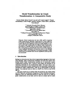
A production models deletion and addition of edges and nodes, carried out in the order just mentioned, i.e., first deletion and then addition. These actions can be represented with two matrices for edges (eE , rE ) and two vectors for nodes (eN , rN ), which can be calculated as:2 e = L (L R) = L R and r = R (L R) = R L. Fig. 2 shows a rule that creates a communication channel between two clients connected to the same server. The deletion matrix eE (and vector eN ) is zero, while the addition matrix rE has a unique non-zero element at position (2, 3) and the addition vector for nodes is zero. From previous definitions, a number of conditions are immedi-

1: S

1: S create channel

2: C

3: C

2: C

(a)

3: C

(b)

Fig. 2. (a) Create Channel Rule (b) Matrix Representation of Rule (only for edges).

ate (see next proposition). The first two state that elements cannot be rewritten (erased and created or vice versa) by a rule application. This is a consequence of the way in which matrices e and r are calculated.3 The last two conditions say that if an element is in the RHS, then it is not deleted, and that if the element is in the LHS, it is not created. Proposition 2. Let p : L → R be a production, the following identities hold for both edges and nodes: r e = r, e r = e, R e = R, L r = L. Finally we are ready to characterize a production p : L → R using deletion and addition matrices, starting from its LHS: R = r ∨ e L (for both edges and nodes). It could be the case that the production erases a node but leaves some incident edges (dangling edges). Some conditions have to be imposed on matrices and vectors of nodes and edges to keep compatibility when a rule is applied (i.e., to avoid dangling edges): 1. An incoming edge cannot be added to a node that is going° to be deleted°or, using the ° ° °¡ ¢t ° norm, °rE ¯ eN °1 = 0. Similarly, for outgoing edges: ° rE ¯ eN ° = 0. Note 1

how, vector eN has a 1 in position i, if the node has to be deleted. Row i in matrix rE depicts the outgoing edges for node i, and has a 1 in column j if edge (i, j) has E to be added. Therefore vector rE ¯ eN contains elements (∨nj=1 rij ∧ eN j )i∈{1,...,n} with a 1 in position i, if there is some newly added edge from node i to some node j which is deleted by the production. The transposition of rE checks for new edges starting from deleted nodes. 2

3

Superindices E and N shall be omitted if, for example, the formula applies to both cases or if it is clear from context which we refer to. Moreover, the and operator (∧) will also be omitted. This contrasts with the DPO approach, in which edges and nodes can be rewritten in a single rule. This can be useful to forbid the rule application if the dangling condition is violated. Section 3 explains how to deal with dangling edges in this approach.

2. Deleting a node with some incoming edge is forbidden, edge is° not deleted as °³ if the ° ° ´t ° ° ° E E N° E well: °e L ¯ e ° = 0. For outgoing edges: ° eE L ¯ eN ° ° = 0. Matrix ° 1 1

eE LE contains the edges in the rule’s LHS that are not deleted, therefore eE LE ¯ eN results in a vector with a one in position i if some node j is deleted and has an incident edge coming from i (and the edge is not deleted). The transposition of eE LE checks for outgoing edges from deleted nodes. 3. It is not possible to add an incoming°edge to³ a node ´° which is neither present in the ° ° LHS nor added by the production: °rE ¯ rN LN ° = 0. Similarly, for edges 1 °¡ ¢ ³ ´° t ° ° starting in a given node: ° rE ¯ rN LN ° = 0. In this case, rN LN is a vector 1 containing a 1 in position i if node i does not belong to the LHS and is not going to be added. 4. It is not possible for an edge to reach not belong to the LHS °³a node´which ³ does ´° ° ° and which is not going to be added: ° eE LE ¯ rN LN ° = 0. For outgoing 1 °³ ° ´t ³ ´° ° E E E N N E ° ° edges: ° e L ¯ r L ° = 0. In this case, e L is a matrix with a 1 in 1 the edges that are in the LHS and not deleted. Thus we arrive naturally at the next proposition: Proposition 3. Let p : L ³ → R be ´a production, if previous conditions in items 1-4 are ³ ´ fulfilled then RE = rE ∨ eE LE and RN = rN ∨ eN LN are compatible. ° ° which is easily proved, as we have to check that °(M ∨ M t ) ¯ N °1 = 0, with ³ ´ M = rE ∨ eE LE and N = rN eN ∨ LN . Therefore, ·³ ´ ³ ´t ¸ h ³ ´i ¡ ¢ M ∨ M t ¯ N = r E ∨ e E LE ∨ r E ∨ e E LE ¯ rN eN ∨ LN = · ´t ¸ ³ ´ ¡ ¢t ³ = r E ∨ e E LE ∨ r E ∨ e E LE ¯ e N ∨ r N LN (1) Conditions in items 1-4 are taken from this identity. For the rule in Fig. 2, it is easy to check that (RE , RN ) are compatible, as vector N has all elements equal to zero (because eN and LN are zero). Up to now we have assumed that when operating with matrices and vectors these had the same size, but in general matrices and vectors represent graphs with different sets of nodes or edges, although probably with some common subsets. Moreover, the elements in both matrices can appear in a different order. An operation called completion modifies matrices (and vectors) to allow some specified operation. Suppose we want to operate with two matrices representing the edges of two graphs (a similar operation can be defined for vectors of nodes). In this way, first a common subset C of elements are identified, and it is moved up in the matrices, maintaining the order. Then, the common subset is sorted in the second matrix to obtain the same order as in the first one. Then,

the elements present in the first matrix but not in the second one are added to the second one (i.e. rows and columns of zeros), sorted like in the first one. Similarly, the elements present in the second matrix but not in the first one are added to the first one (i.e. rows and columns of zeros), sorted like in the second one. For example, if we have to operate the graph in Fig. 1 with the LHS of rule in Fig. 2, then the matrix of edges and the vector of nodes of the rule have to be enlarged. If we identify nodes and edges with the same label, we get the following result:     0000 1 1 1 1 0 0 0 2 1 2 0N     L0E CC =  1 0 0 0 3  ; LCC =  1 3  0000 4 0 4 where an additional column and row has been added to the edge matrix and an additional element has been added to the nodes vector. In this case, the matrices for the graph in Fig. 1 remain the same. Note how, if we had assumed other identification of nodes in the different graphs, the completion procedure would have produced a different result. Once the matrices and vectors of the two graphs are completed, we can define any graph transformation (i.e. any morphism on simple digraphs) as two boolean functions (for the edges matrix and for the nodes vector, which we have modelled with e and r). These functions may change arbitrarily 0’s and 1’s in the matrix of edges and vector of nodes (and thus we have to check compatibilty after their application). 2.2 Concatenation, Permutations and Minimal Initial Digraph It is possible to define sequences of rules and the order in which they are to be applied. Definition 2 (Concatenation) Given a set of productions {p1 , . . . , pn }, the notation sn = pn ; pn−1 ; . . . ; p1 defines a sequence of productions establishing an order in their application, starting with p1 and ending with pn . A concatenation is said to be coherent if actions carried out by one production do not prevent4 the application of those coming afterwards. Fig. 3 shows more rules for the example. Messages are depicted as self-loops, which can be sent through channels. For example sequence remove channel; send; message ready; create channel is coherent, as link (2, 3) is created by the first rule (create channel), used by rule send and then deleted by the last rule. We assume an identification of nodes in the different rules having the same numbers, but other combinations could be studied as well.5 The conditions for coherence of a concatenation of two rules s2 = p2 ; p1 are: E 1. The first production – p1 – does not delete any edge used by p2 : eE 1 L2 = 0. E 2. p2 does not add any edge used, but not deleted, by p1 : r2E LE 1 e1 = 0. E E 3. No common edges are added by both productions: r1 r2 = 0. 4 5

Potentially, because no actual application of productions to a host graph is considered. Hence, completion is not unique – there may exist several ways to identify nodes across productions – depending on how rules are defined or the operation to be performed.

1: S

1: S

2: C

1: S

1: S 1: S

message ready

connect2 server

2: C

1: S

1: S

2: C 2: C

2: C

send

3: C

2: C

3: C

1: S

1: C

server down

1: S remove channel

client down

2: C 3: C

2: C 3: C

Fig. 3. Additional Rules for the Client-Server Example

The first condition is needed because if p1 deletes one edge used by p2 , then p2 is not applicable. The last two conditions are needed in order to obtain a simple digraph (with at most one edge in each direction between two nodes). Applying the first two identities in proposition 2, the three previous equalities can be transformed into E E E E R1E eE 2 r2 ∨ L2 e1 r1 = 0 and similar for nodes. Our objective is to obtain a closed formula to represent these conditions for the case with n productions. For this purpose, we introduce a graphical notation for boolean equations: a single arrow means ∧, while a fork (more than one arrow starting in the same node) stands for ∨. These diagrams are useful to understand how the formulas change depending on the number of productions. As an example, the representation of coherence equations for two productions (for edges) is shown in Fig. 4(left). The figure also shows the equations for three and five productions.

Fig. 4. Graph for Sequence of Length 2 (left), 3(middle) and 5(right).

Analysing the graphs for sequences of increasing size, we arrive at the following theorem concerning sequences of arbitrary size. The proof is not included here, it can be found at [10]. Theorem 1 (Sequence Coherence). The concatenation sn = pn ; . . . ; p1 is coherent if n _ ¡

¢ Ri 5ni+1 (ex ry ) ∨ Li 4i−1 (ey rx ) = 0 1

(2)

i=1

where 4tt10

(F (x, y)) =

t1 _ y=t0

Ã

t1 ^ x=y

! (F (x, y))

; 5tt10

(G(x, y)) =

t1 _ y=t0

Ã

y ^

x=t0

! (G(x, y))

E.g., sequence s1 = remove channel; send; message ready; create channel is coherent but send; message ready; remove channel is not, because the first production (remove channel) deletes edge (2, 3) needed by send one step afterwards. The resulting matrix of the coherence formula has a one in such position and zeros elsewhere. In this way, the resulting matrix of the formula is useful to indicate where the potential coherence problems are. On the other hand, sequence s2 = remove channel; send; create channel is coherent, but it is worth stressing that edge (2, 2) needs to be supplied by the host graph, because rule send needs a self loop representing a message and we know that such element is not added by any rule before send. Altogether, coherence allows the grammar designer to check dependencies between rules, and to realize possible conflicts, some of which can be solved if the initial graph provides enough edges and nodes. This is related to the notion of minimal initial digraph, which is a graph containing the necessary nodes and edges for a rule (or sequence) to be applicable. Theorem 2 (Minimal Initial Digraph). Given a coherent concatenation of productions sn = pn ; . . . ; p1 , its minimal initial digraph is defined by: Mn = 5n1 (rx Ly ). One graph is easily Wn obtained which contains enough nodes and edges to execute a coherent sequence: i=1 Li . However, this graph can be made smaller, so for example, for production p1 we only include in Mn elements which are in the LHS, but not added. In a similar way, for p2 we include elements in its LHS if they are not added by p2 nor p1 . Therefore, we have Mn = (r1 L1 ) ∨ (r1 L2 )(r2 L2 ) ∨ · · · ∨ (r1 Ln ) · · · (rn Ln ), which is the expanded form of 5n1 (rx Ly ). Note how, we assume a given identification of nodes and edges in the different productions of the sequence, that is, a certain way of completing each matrix. The calculation of the minimal initial digaph for sequence s2 = remove channel; send; create channel is shown in Fig.5 as an example. 1: S

1: S

1: S

1: S

1: S

1: S

= 2: C 3: C

2: C 3: C

2: C 3: C

2: C 3: C

2: C 3: C

r L

r L

r L

r L

r L=r L

1 1

2 2

1 2

1 3

2 3

2: C 3: C

3 3

Fig. 5. Minimal Digraph for Sequence s2 .

The image of a concatenation sn = pn ; . . . ; p1 (please, refer to [10]) Wn almost can be seen as a production sn = (rs , es ), where rs = 4n1 (ex ry ) and es = i=1 ei , i.e., n ^ sn (Mn ) = (ei Mn ) ∨ 4n1 (ex ry ) = rs ∨ es Mn (3) i=1

However, in this case, it is not true that rs es = rs , which in particular implies that it is important to delete elements (apply es ) before addition takes place (rs application). The following result states conditions to keep coherence in case of permuting one production inside a sequence [10]. Theorem 3 (Production Permutations). Consider coherent productions tn = pα ; pn ; pn−1 ; . . . ; p1 and sn = pn ; pn−1 ; . . . ; p1 ; pβ and permutations φ and δ.

³ ´ ³ ´ n E E ∨ RE 5n eE r E = 0. 1. φ (tn ) is coherent if: eE α 51 rx Ly α x y 1 ³ ´ ³ ´ n E eE ∨ r E 4n eE RE = 0. 2. δ (sn ) is coherent if: LE 4 r x y x y 1 1 β β where φ advances the last production to the front, that is, moves the left-most rule to the right n − 1 positions in a sequence of n rules. Thus, φ has associated permutation φ = [ 1 n n−1 . . . 3 2 ]. In a similar way, δ delays the first production n−1 positions in a sequence of n rules, moving it to the last position. Thus, δ = [ 1 2 . . . n−1 n ]. For sequence t2 = send; create channel; remove channel, φ(t2 ) = create channel; remove channel; send is coherent. G-congruence guarantees that two coherent and compatible concatenations have the same output starting with G as minimal initial digraph. The conditions to be fulfilled are known as Congruence Conditions (CC). A coherent and compatible concatenation sn and a coherent and compatible permutation of it, σ (sn ), which besides have the same minimal initial digraph G (G-congruent) are potentially sequential independent. For advancement and delaying of productions, the congruence conditions are (see [10]): (ex ry ) ∨ rn ∇n−1 (rx Ly ) = 0 CC (φ, sn ) = Ln ∇n−1 1 1 n n CC (δ, sn ) = L1 ∇2 (ex ry ) ∨ r1 ∇2 (rx Ly ) = 0

(4) (5)

For sequence s = send; create channel; remove channel, CC(φ, s) = 0, therefore we obtain the same result by advancing send twice. As s and φ(s) have the same initial digraph (the one in Fig. 5, plus edge (2, 3)), they are potential sequential independent. Symbol ⊥ denotes potential sequence independence, thus we can write send⊥(create channel; remove channel) in previous example. Note that it is possible to check sequential independence between a rule and a sequence, in contrast with results in the algebraic-categorical approach.

3 Match, Extended Match and Production Transformation Matching is the operation of identifying the LHS of a rule inside a host graph. This identification is not necessarily unique, thus becoming a source of non determinism. Definition 3 (Match) Given a production p : L → R and a simple digraph G, any m : L → G total injective morphism is known as a match (for p in G). Recalling the notion of completion, a match can be interpreted as one of the possible ways to complete L in G. We do not explicitly care about types or labels in our matrices (“S” and “C” in the examples), but this can be thought as restrictions for the completion procedure, which cannot identify elements with different types. Fig.6(a) displays a production p and a match m for p in G. It is possible to close the diagram, making it commutative (m∗ ◦ p = p∗ ◦ m), using the pushout construction [5] on category Pfn(Graph) of simple digraphs and partial functions (see [9]). This categorical construction for relational graph rewiting is carried out in [9] in their Theorem 3.2 and Corollary 3.3. Proposition 3.5 in [9] gives a sufficient condition to decide if a given rewriting square like the one in Fig.6(a) can be closed.

L L

p

/R

m

m∗

²

G

²

p∗

/H

p

/R

m

²

G

²

p∗

/H m∗ ε

mε

²

G

m∗

p b∗

² /H

p

L- GG

-- GG m -- GGGG # -iL iG G mG - xx -x xxmε ² {xx --L × GF FF -- pb FF FF m b # ¹² G

/RG GG ∗ GGm GG iR G# p∗ /H ² { / R×H

iH m∗ ε ∗

m b ∗

p b

# ² /H

Fig. 6. (a) Production plus Match. (b) Neighbourhood. (c) Extended Match and Production.

Definition 4 (Direct Derivation) Given p : L → R and m : L → G as in Fig.6(a), d = (p, m) is called a direct derivation with result H = p∗ (G). If a concatenation sn = pn ; . . . ; p1 is considered together with the set of matchings mn = {m1 , . . . , mn }, then dn = (sn , mn ) is a derivation. When applying a rule to a host graph, the main problem to concentrate on is that of so-called dangling edges, which is differently addressed in SPO and DPO. In DPO, if an edge comes to be dangling then the rule is not applicable (for that match), while SPO allows the production to be applied, deleting any dangling edge. In this paper we propose an SPO-like behaviour. Fig.6(b) shows our strategy to handle dangling edges: 1. Morphism m shall identify rule’s left hand side in the host graph. 2. A neighbourhood of m(L) ⊆ G covering all relevant extra elements is selected (performed by mε 6 ), taking into account all dangling edges not considered by match m with their corresponding source and target nodes. 3. Finally, p is enlarged (through operator Tε , see definition below) erasing any otherwise dangling edge. Definition 5 (Extended Match) Given a production p : L → R, a host graph G and a match m b : L × G → G is a morphism whose image S : L → G, the extended match m is m (L) ε, where ε is the set of dangling edges and their source and target nodes. Coproduct (see Fig.6(c)) is used for coupling L and G, being the first embedded def

def

into the second by morphism m. We use the notation L = mG (L) = (mε ◦ m) (L) i.e., extended digraphs are underlined and defined by composing m and mε . Example.¤Consider the digraph L, the host graph G and the morphism match depicted on the left side of Fig. 7. On the top right side in the same figure, m(L) is drawn, and mG (L) on the bottom right side. Nodes 2 and 3 and edges (2, 1), (2, 3) and (2, 2) have been added to mG (L). The edges would become dangling in the image “graph” of G by p, p (G). Note how this composition is possible, as m and mε are functions between boolean matrices which have been completed. ¥ Once we are able to complete the rule’s LHS, we have to do the same for the rest of the rule. To this end we define an operator Tε : G → G0 , where G is the original 6

Recall that morphisms are functions on boolean matrices and vectors.

client down

L 2: C

m H

1: S

G 2: C

3: C

4: C

m*

m (G)

3: C

client

4: C down

*

1: S 2: C

4: C G

ε

1: S

1: S 3: C

3: C

m (L) = (m o m) (L)

ε

H

1: S

2: C

ε

1: S

m*

ε

2: C

m (L)

3: C

m G

R

4: C

2: C

3: C

Fig. 7. Matching and Extended Match.

grammar and G0 is the grammar transformed once Tε has modified the production. The notation that we use from now on is borrowed from functional analysis [1]. Bringing this notation to graph grammar rules, a rule is written as R = hL, pi (separating the static and dynamic parts of the production) while the grammar rule transformation including matchings is: R = hmG (L) , Tε pi. Proposition 4. With notation as above, production p can be extended to consider any dangling edge, R = hmG (L) , Tε pi. Proof ¤What we do is to split the identity operator in such a way that any problematic element is taken into account (erased) by the production. In some sense, we first add elements ∗ −1 to p’s LHS and afterwards enlarge p to erase­them. Otherwise ¡ −1 ¢ ®stated, mG = Tε and Tε∗ = m−1 , so in fact we have R = hL, pi = L, T ◦ T p = hm (L) , T ε G ε (p)i = ε G R. The equality R = R is valid strictly for edges. ¥ The effect of considering a match can be interpreted as a new production concatedef

nated to the original production. Let pε = Tε∗ , R = hmG (L) , Tε (p)i = hTε∗ (mG (L)) , (p)i = = p (Tε∗ (mG (L))) = p ; pε ; mG (L) = p ; pε (L)

(6)

Considering the match can be interpreted as a temporary modification of the grammar, so it can be said that the grammar modifies the host graph and – temporarily – the host graph interacts with the grammar. If we think of mG and Tε∗ as productions respectively applied to L and mG (L), it is necessary to specify their erasing and addition matrices. To this end, we introduce matrix ε, with elements in row i and column i equal to one if node i is to be erased by p, and zero otherwise (see definition 5). This matrix considers any potential dangling edge. For mG we have that eN = eE = 0, and r = L L (for both nodes and edges), as the production ¢has to add the elements in L that are not present in L. Let pε = ¡ E E E N N E N E eTε , rTε ; eN Tε , rTε , then eTε = rTε = rTε = 0 and eTε = ε ∧ L . Example.¤Consider rules depicted in Fig. 8, in which server down is applied to model a server failure. We have £ ¤ £ ¤ £ ¤ £ ¤ eE = rE = LE = 0 1 eN = 1 1 ; rN = 0 1 ; LN = 1 1 ; RE = RN = ∅

L

server down

1: S

R

m G

down

3: C

4: C

ε

2: C

m* server * H

1: S 2: C

L

L 2: C

3: C

server

1: S down 3: C

R

1: S

ε 2: C

1: S server server down

4: C 2: C

Tε

3: C

down

3: C

R Tε

2: C 3: C

Fig. 8. Full Production and Application.

Once mG and operator Tε have been applied, the resulting matrices are       · ¸ 000 1 000 1 000 1 00 2 1 0 0 2 r E =  1 0 0 2  ; LE =  1 0 0 2  ; R E = ; eE Tε = 00 3 100 3 100 3 100 3 Matrix rE , besides edges added by the production, specifies those to be added by mG to the LHS in order to consider any potential dangling edge (in this case (2, 1) and (3, 1)). As neither mG nor production server down delete any element, eE = 0. Finally, pε removes all potential dangling edges (check out matrix eE Tε ) but it does not add any, so rTEε = 0. Vectors for nodes have been omitted.¥ ´ ³ E Let Tε∗ = Tε∗ N , Tε∗ E be the adjoint operator of Tε . Define eE ε and rε respectively as the erasing and addition matrices of Tε (p). It is clear that rεE = rE = rE and E E eE ε = e ∨ ε L , so ­ ® ¡ ¢ E E E E E = rεE ∨ eE L = RE = LE ,³Tε (p) ´ ε L = r ∨ e ∨ εL E E E E E E E =r ∨ ε∨L e L =r ∨e εL ­ E E ¡ E ¢® ­ E E ® E The previous = ε L , p , which proves ³ identities´show that R = L , Tε p that Tε∗ = Tε∗ N , Tε∗ E = (id, ε). Summarizing, when a given match m is considered for a production p, the production itself is first modified in order to consider all potential dangling edges. m is automatically transformed into a match which is free from any dangling element and, in a second step, a pre-production pε is appended to form the concatenation pb∗ = p∗ ; p∗ε

4 Revision and Extension of Basic Concepts In this section we brush over all concepts and theorems introduced in section 2, completing them by considering matchings. Let sn = pn ; . . . ; p1 be a concatenation. As there is a match for every production in the sequence, it is eventually transformed into s∗n = pn ; pε,n ; . . . ; p1 ; pε,1 . Fig.9 displays the corresponding derivation. For compatibility, the main difference when considering matchings is that the sequence is increased in the number of productions so it shall be necessary to check more conditions.

L1

pε,1

mG,1

²

G

/ L1

L1 CC CC CC m1 CC ! ² / Gε,1

p∗ ε,1

p1

p

ε,2 / R1 / L2 L2 L2 AA CC CC AA CC AA mG,2 m2 CC AA ! ² Ã ² / G1 / Gε,2

p∗ 1

p∗ ε,2

p2

p∗ 2

/ ...

/ ...

Fig. 9. Productions and ε-productions in a Concatenation.

4.1 Initial Digraph Set Concerning the minimal initial digraph, one may have different ways of completing the rule matrices, depending on the matches. Therefore, we no longer have a unique initial digraph, but a set. Definition 6 (Initial Digraph Set) Given sn a sequence, its associated initial digraph set M (sn ) is the set of simple digraphs Mi such that 1. Mi has enough nodes and edges for every production of the concatenation to be applied in the specified order, and 2. Mi has no proper subgraph with previous property ∀Mi ∈ M (sn ). Every element Mi ∈ M (sn ) is said to be an initial digraph for sn . It is easy to see that M (sn ) 6= ∅, ∀sn finite sequence of productions. The initial digraph set contains all graphs that can potentially be identified by matches in concrete host graphs. In section 2.1, coherence was used in an absolute way but now, due to matching, coherence is a property depending on the given initial digraph. Hence, we now say that sn is coherent with respect to initial digraph Mi . For the initial digraph set, we can define the maximal initial digraph as the element Mn ∈ M (sn ) which considers all nodes in pi to be different. This element is unique up to isomorphism, and corresponds to considering the parallel application of every production in the sequence. In a similar way, Mi ∈ M (sn ) in which all possible identifications are performed are known as minimal initial digraphs, which in general are not unique. As an example, left of Fig. 10 shows the minimal digraph set for sequence s2 = remove channel; remove channel, which is not coherent, as the link between two clients is deleted twice. In this way, the initial digraphs should provide two links. It is possible to provide some structure T (sn ) to set M (sn ) (see the right of Fig. 10). Every node in T represents an element of M, and a directed edge from one node to another stands for one operation of identification between corresponding nodes in LHS and RHS of productions of the sequence sn . Node M7 is the maximal initial digraph, as it only has outgoing edges. The structure T is known as graph-structured stack, in our case with single root node. 4.2 Coherence Coherence formulas do not change, except that now there are conditions for all εproductions. When considering the match, coherence is similar to conflict detection in

M1 1: S 2: C

3: C

M4 1: S

M2

M3

1:S

2:C 3:C 4:C 5: S

M6

1:S

2:C 3:C 4:C

M5 1: S

5: S

2:C

M7

1:S

3:C 1:S

3=5 4:C

5:C

4:S

M7

3=6

1=4

M4

M6

1=5 3=4

M5

3=5

M2

2=4 2: C

3: C

4: C

2: C

3: C

4: C

2:C 3:C 5:C 6:C

1=5

M3

2=4 M1

Fig. 10. Initial Digraph Set for s2 = remove channel; remove channel.

critical pairs [5] [6], where an important issue is efficiency [8]. We believe our approach is a contribution in improving the efficiency in finding this kind of conflicts. The functional notation introduced so far can be used to re-enunciate Theorem 1 for coherence, deriving conditions which resemble those of perpendicular vectors and kernel of a function. Let qLi = 41n−1 (rx ey ) and qRi = 5ni+1 (ex ry ), then sn = pn ; . . . ; p1 is coherent if hLi , qLi i = hRi , qRi i = 0. In addition, when the host graph is not considered, if nodes are identified across rules, it can be the case that some dangling edge appears in the concatenation. For example, given p2 ; p1 , suppose that rule p1 uses but does not delete edge (4, 1), that rule p2 specifies the deletion of node 1 and that we have identified both nodes 1. It is mandatory to add one ε-production pε,2 to the grammar, which conceptually is of a different nature than those previously discussed. The latter dangling edges appear in the context where the rule is applied, but not in other rules. We have an unavoidable problem of coherence between p1 and pε,2 if we wanted to advance the application of pε,2 to p1 . Hence, we split the set of edges deleted by ε-productions into two disjoint classes: – External. Any edge not appearing explicitly in the grammar rules, i.e., edges of the host graph “in the surroundings” of the actual initial digraph. Examples are edges (2, 1) and (3, 1) in Fig.8. – Internal. Any edge used or appended by a previous production in the concatenation. One example is the previously mentioned edge (4, 1). ε-productions can be classified accordingly in internal ε-productions if any of its edges is internal and external ε-production otherwise. External ε-productions cannot be considered during rule specification which, in turn, may spoil coherence, compatibility, etc. One way to handle this problem is to check the conditions under which all ε-productions can be advanced to the front of the sequence. Given a host graph G in which sn – coherent and compatible – is to be applied, and assuming a match which cε , identifies sn ’s actual initial digraph (Mn ) in G, we check whether for some m b and T which respectively representDall changes to be done to Mn and all modifications to sn , E c it is correct to write Hn = m b (Mn ) , Tε (sn ) , where Hn would be the piece of the final state graph H corresponding to the image of Mn . Example.¤Let s2 = p2 ; p1 be a coherent and compatible concatenation. Using operators we can write H = hmG,2 ¡ (hm ¢ G,1 (M2 ) , Tε,1 (p1 )i) , Tε,2 (p2 )i, which is equivalent to H = p2 ; pε,2 ; p1 ; pε,1 M2 , with actual initial digraph twice modified M2 = mG,2 (mG,1 (M2 )) = (mG,2 ◦ mG,1 ) (M2 ).¥

Definition 7 (Exact Derivation) Let dn = (sn , mn ) be a derivation with actual initial digraph Mn , concatenation sn = pn ; . . . ; p1 , matches mn = {mG,1 , . . . , mG,n } and cε such ε-productions {pε,1 , . . .D, pε,n }. It is an exact b and T E derivation if there exist m cε (sn ) . that Hn = dn (Mn ) = m b (Mn ) , T Previous equation might be satisfied if once all matches are calculated, the following identity holds: pn ; pε,n ; . . . ; p1 ; pε,1 = pn ; . . . ; p1 ; pε,n ; . . . ; pε,1 . Equation (3) allows cε and m us to consider a concatenation almost as a production, justifying operators T b and our abuse of the notation (recall that brakets apply to productions and not to sequences). Proposition 5. With notation as before, if pε,j ⊥ (pj−1 ; . . . ; p1 ), ∀j, then dn is exact. Proof cε modifies the sequence adding a unique ε-production, the composition 7 ¤Operator T of all ε-productions pε,i . To see this, if one edge is to dangle, it should be eliminated by the corresponding ε-production, so no other ε-production deletes it unless it is added by a subsequent production. But by hypothesis there is sequential independence of every pε,j with respect to all preceeding productions and hence pε,j does not delete any edge used by pj−1 , . . . , p1 . In particular no edge added by any of these productions is erased. In definition 7, m b is the extension of the match m which identifies the actual initial digraph in the host graph, so it adds to m (Mn ) all nodes and edges to distance one to cε shows that m nodes that are going to be erased. A symmetrical reasoning to that of T b is the composition of all mG,i .¥ With definition 7 and proposition 5 it is feasible to get a concatenation where all εproductions are applied first, and all grammar rules afterwards, recovering the original concatenation. Despite some obvious advantages, all dangling edges are deleted at the beginning, which may be counterintuitive or even undesired. For example, if the deletion of a particular edge is used for synchronization purposes. The following corollary states that exactness can only be ruined by internal ε-productions. Let sn be a sequence to be applied to a host graph G and Mk ∈ M (sn ). Corollary 1. With notation as above, assume there exists at least one match in G for Mk that does not add any internal ε-production. Then, dn is exact. Proof (sketch) ¤All potential dangling elements are edges surrounding the actual initial digraph. It is thus possible to adapt the part of the host graph modified by the sequence at the beginning, so applying proposition 5 we get exacteness.¥

5 Conclusions and Future Work In this paper we have presented a new approach to simple digraph transformation based on an algebra of boolean matrices. We have shown some results (coherence, minimal 7

Given a sequence of productions, their composition is one production which performs the same operations, see [10] for the formal definition.

initial digraphs, permutation, G-congruence) that can be calculated on the graph transformation system, independent of the host graph. We have introduced the match, and how to handle dangling edges by generating ε-productions which are applied previous to the original rule in order to delete dangling edges. We believe that the main difference of our approach with respect to others is that we use boolean operators to represent graph manipulations. Other approaches such as DPO and SPO use a categorical representation of the operations, which, on the one hand makes the approach more general, but on the other, makes bigger the gap between specification and implementation on tools. In addition, we believe that concepts like initial digraph, coherence, arbitrary sequences of finite length are easier to express and study in our framework than using category theory. Concerning additional related work, the relational approach of [9] uses also exclusively a categorical approach for operations. Other approaches such as logic-based [12], algebraic-logic [2], relation-algebraic [7] are more distant from ours. With respect to future work, we are working on application conditions, studying the structure of M(sn ), bringing to our framework techinques from Petri nets, considering more general types of graphs and implementing the current concepts in a tool. Acknowledgements: This work has been sponsored by the Spanish Ministry of Science and Education, project TSI2005-08225-C07-06. The authors would like to thank the referees for their useful comments.

References 1. Braket notation intro: http://en.wikipedia.org/wiki/Bra-ket notation. 2. Courcelle, B. 1990. Graph Rewriting: An Algebraic and Logic Approach Handbook of Theoretical Computer Science, Vol. B. pp.: 193-242. 3. Ehrig, H. 1979. Introduction to the Algebraic Theory of Graph Grammars. In V. Claus, H. Ehrig, and G. Rozenberg (eds.), 1st Graph Grammar Workshop, pages 1-69. LNCS 73. 4. Ehrig, H., Heckel, R., Korff, M., L¨owe, M., Ribeiro, L., Wagner, A., Corradini, A. 1999. Algebraic Approaches to Graph Transformation - Part II: Single Pushout Approach and Comparison with Double Pushout Approach. In [11] Vol.1, pp.: 247-312. 5. Ehrig, H., Ehrig, K., Prange, U., Taentzer, G. 2006. Fundamentals of Algebraic Graph Transformation. Springer. 6. Heckel, R., K¨uster, J. M., Taentzer, G. 2002. Confluence of Typed Attributed Graph Transformation Systems. Proc. ICGT’2002. LNCS 2505, pp.: 161-176. Springer. 7. Kahl, W. 2002. A Relational Algebraic Approach to Graph Structure Transformation Tech.Rep. 2002-03. Universit¨at der Bundeswehr M¨unchen. 8. Lambers, L., Ehrig, H., Orejas, F. 2006. Efficient Conflict Detection in Graph Transformation Systems by Essential Critical Pairs. Proc. GT-VMT’06, to appear in ENTCS (Elsevier). 9. Mizoguchi, Y., Kuwahara, Y. 1995. Relational Graph Rewritings. Theoretical Computer Science, Vol 141, pp. 311-328. 10. P´erez Velasco, P. P., de Lara, J. 2006. Towards a New Algebraic Approach to Graph Transformation: Long Version. Tech. Rep. of the School of Comp. Sci., Univ. Aut´onoma Madrid. http://www.ii.uam.es/∼jlara/investigacion/techrep 03 06.pdf. 11. Rozenberg, G. (managing ed.) 1999. Handbook of Graph Grammars and Computing by Graph Transformation. Vol.1 (Foundations), Vol.2(Applications, Languages and Tools), Vol.3., (Concurrency, Parallelism and Distribution). World Scientific. 12. Sch¨urr, A. Programmed Graph Replacement Systems. In [11], Vol.1, pp.: 479 - 546.