technique to smooth sensor data, but not suited for com- ... Permission is granted for indexing in the ACM Digital Libra
Poster: Maxima Estimation in Spatial Fields by Distributed Local Polynomial Regression Reiner Jedermann
Henning Paul
Walter Lang
Institute for Microsensors, -actuators and systems (IMSAS) University of Bremen, Germany +49 (0)421 218 - 62 603
Department of Communications Engineering University of Bremen, Germany +49 (0)421 218 - 62399
Microsystems Center Bremen (MCB) University of Bremen, Germany +49 (0)421 218 - 62 601
[email protected]
[email protected]
[email protected]
Abstract Identifying the location of field maxima is a crucial task in environmental monitoring. A modified local polynomial regression method was applied to find maxima in between the sensor nodes. The method is well suited for a distributed implementation.
Keywords Spatial field reconstruction; wireless sensor networks; local polynomial regression; in-network processing
1
Introduction
In several wireless sensor network applications, e.g. monitoring the temperature in a refrigerated container [2] or truck [3], the observed physical property varies over space. Crucial information is the location of field maxima or so-called hot-spots. The location of hot-spots is not known in advance, so they will most likely be found in between the sensor nodes (SNs). We present a solution to this problem to estimate the coordinates of field maxima. The algorithm requires only information from the close neighborhood of SNs and is therefore well suited for local in-network processing with a reduced communication volume.
2
Algorithm
The algorithm is based on an extension to the method of local polynomial regression (LPR) [1], which is a common technique to smooth sensor data, but not suited for compressed data transmission in its original form. The target point is locally fitted by a second order polynomial in our approach. Neighboring data points are weighted by a kernel function with limited support, i.e., only points within a short radius λ have a non-zero influence. We assume that each SN knows its own position coordinates and is able to query the current (temperature) measurement
International Conference on Embedded Wireless Systems and Networks (EWSN) 2016 15–17 February, Graz, Austria © 2016 Copyright is held by the authors. Permission is granted for indexing in the ACM Digital Library ISBN: 978-0-9949886-0-7
and the coordinates of its neighbors within λ, if necessary, over an intermediate hop. In order to test for low communication volumes, the input data for each SN was furthermore limited to information from its kN =15 nearest neighbors. The algorithm consists of the following three steps: Step 1 (Smoothing): Each SN queries its neighbors and smooths its own data locally. This first step is necessary to avoid the search algorithm getting stuck in a local maximum caused by measurement noise. Step 2 (Climbing search): The search for the SN with the highest values is started by assigning a handle to 9 SNs on a 3 x 3 grid. The handle is passed to the neighbor with the highest smoothed value. If an SN receives two or more handles and has no neighbor with a higher value, it is considered as a significant maximum (Figure 1). Step 3 (Inter-node search): The selected SNs of step 2 scan their proximity for higher values based on an LPR reconstruction of the field by heuristic optimization. All necessary data have already been transferred during step 1. The LPR prediction is calculated for two points with a small position offset in x-direction of ∆x =±0.03 m. The maximum of a parabola through these total three points is calculated, giving a fourth point. The maximum of the four points is taken as new estimation of the field maxima coordinates. The process is repeated two times for the x and y coordinates.
Figure 1. Example of climbing search. Position of sensors (black dots), climbing steps (blue), maxima of reference data (green circles) and estimated maxima (red crosses).
223
3
Test Data and Implementation
The algorithm is suited for various types of spatial sensor data, e.g. estimation of the center of chemical spills in a lake, or the location of hot-spots from open field climate measurements or spatial temperature measurements in refrigerated warehouses. In order to test the accuracy of the algorithm, the exact locations of the field maxima have to be known as a reference, which is normally not the case in real-world sampling data. Furthermore, the simulation should be repeated for different locations of the SNs and different instances of the measurement noise, which is only feasible with simulated data. The data set was generated by COMSOL for the temperature field of three heat sources in a water basin of size 2 m·2 m, including different physical effects such as heat transfer by diffusion and horizontal advection. Gaussian noise was added to a randomly selected set of SN positions (Figure 2).
Figure 2. Noise-free test data (colored surface) and smax =100 measurements (red crosses) with σNoise =0.1.
Figure 3. Average absolute error of the estimation of the two highest maxima as a function of the number of sensors smax and of noise σNoise .
5
Conclusions
The simulation framework consisted of a set of MATLAB scripts, which handle the data exchange between the SNs and graphical display of the results, and Java code. Each SN and its data processing were represented by a Java object. In addition to simulation on a workstation, the Java code was tested on a SunSpot sensor node from Oracle equipped with a 400 MHz ARM CPU. The estimation of the maxima required 78 ms on the SNs that were nearest to the field maxima and 7 ms on the other SNs.
We showed that the algorithm is well suited for distributed implementation by simulation, testing of one JAVA instance on real sensor node hardware, and evaluation of the communication requirements. The number of SNs required for maxima estimation with sufficient accuracy depends on the number of field maxima. In our test scenario with three maxima, 150 SNs were sufficient for a reliable estimation, provided that the amplitude (standard deviation) of the noise is not greater than 10% of the peak-to-peak range of the observed values.
4
6
Results
For noise-free data and smax =500 SNs, the average absolute error of the predicted location of the first two maxima was only 0.56% of the lateral length of the observed area. The error increased with higher noise and a lower number of SNs (Figure 3). Prediction errors were not only due to the lack of accuracy of our LPR model. The low number of SNs provided insufficient information for accurate maxima estimation; further inaccuracies were caused by noise. In a typical scenario with σNoise =0.1, equivalent to 10% of the maximum temperature change, a stable estimation was possible for smax =200. In 98.7% of the total 1000 simulation runs the first and the second maxima were correctly estimated with an average error of 2.49% of their location and 5.9% of their height. For smax