Maximum Entropy: A Special Case of Minimum Cross-entropy Applied to Nonlinear Estimation by an Artificial Neural Network Joseph C. Park*
2d3D Incorporated, 2003 North Swinton Avenue, Delray Beach, FL 33444 Salahalddin T. Abusalah÷
University of West Florida, Department of Electrical and Computer Engineering, Pensacola, FL 32514 The application of cross-entropy information processing optimizations to artificial neural network (ANN) training can provide decreased sensitivity to accelerated learning rates as well as insights into the information processing structure of the network. In order to assess the cross-entropy between the desired training goal and the evolving state of network information at each training step, the probability distributions of the network output at each step, as well as that of the desired network output must be available. However, if the input training data is not expressible as a closed form function, analytic representation of the network output distribution may be impossible, excluding the application of cross-entropy measures to many higher-dimensional, real-world problems. In such cases the network may be trained according to entropy maximization of the output training distribution. To illustrate this, a perceptron is detailed which estimates orthogonal basis function coefficients of a highly nonlinear set of oceanographic data based on entropy maximization. Use of the maximum entropy cost-function obviates the need for explicit determination of the network output probability distributions, while retaining the desirable functionality of information-theoretic network organizations.
1. Introduction
Artificial neural networks (ANNs) constitute a class of computational architectures capable of processing, storing, and predicting complex informational systems. These networks are comprised of simple, multiply interconnected computational units, each of which performs a summation that is then applied to a nonlinear transfer function for output. In * Electronic
÷ Electronic
mail address:
[email protected]. mail address:
[email protected].
Complex Systems, 11 (1997) 289–307; ” 1997 Complex Systems Publications, Inc.
290
J. C. Park and S. T. Abusalah
order for an ANN to arrive at a computationally useful structure (in terms of the interconnection weight-states) the network must either be trained to recognize the relevant feature information, or have incorporated into its processing structure a rule-base which dictates the network evolution. In this paper we focus on the former class wherein a feedforward (nonrecurrent) ANN is trained to recognize a multivariate oceanic environmental data set. The training process is essentially a directed organization based on an error (or uncertainty) minimization which can be recognized as a process of informational entropy minimization. In general terms, training constitutes a minimization of cross-entropy (or mutual information) between the distributions of the actual and desired network outputs. Much of the previous work connecting neural networks and information theory simply applied the ANN as an analysis tool for classical statistical estimation. Either the ANN was employed to implement maximum entropy statistical estimation for probability distribution functions (PDFs) based on incomplete information in constrained optimization problems, to multidimensional spectral estimation, or to provide signal reconstruction [1–4]. Other work applied the ideas of information theory to assay the inherent effectiveness of ANN architectures in terms of information content [5]. Another body of research explored methods to explicitly train ANNs in the information-space of the network output variables [7–11], instead of training based on the parametric error of the outputs themselves, and established that such an approach can allow the network to tolerate increased learning rates without divergence. These information-space training scenarios are based on the minimization of cross-entropy (mutual information content) between the desired output distribution and the current distribution of the network output. This requires that probability distributions for both the network output at each training step and for the output training sets are known. While the latter presents no difficulty, specification of the network output PDF at each training step may be analytically intractable in cases where the input training set PDF is not expressible in closed form.1 This situation encompasses many real-world dynamical systems wherein the underlying physics are high-dimensional and exhibit significant complexity. Therefore, it is of significant practical interest to remove this restriction so that any measurable physical process can be amenable to an ANN estimation which employs the information1 One could argue that an analytical representation is not required, it is possible to simply estimate the distribution at each learning step for each output unit through relative frequency computations. However, such a computational burden is not very attractive when considering the typically intensive numerical load of an ANN with significant complexity, as well as the introduction of additional uncertainties by virtue of the PDF estimation.
Complex Systems, 11 (1997) 289–307
Maximum Entropy: A Special Case of Minimum Cross-entropy
291
theoretic training measures. Following this assertion, and in contrast to the previous body of work exploring the connections between information theory and ANN training, the focus of this paper is to explicitly detail application of the maximum entropy principle as the cost-function of gradient-descent training in the information-space of the network output parameters, thereby enabling the information-theoretic cost functions as viable alternatives to classical parametric cost functions in cases where the input distribution is not analytically accessible. We proceed by demonstrating that application of cross-entropy as a cost function in ANN training is a general case of entropy minimization, while the entropy maximization constitutes a special case. This distinction is made clear in section 1.1. 1.1 Information measures and entropy maximization
To clarify the relationship between minimization of cross-entropy and maximization of entropy, examine the classic definition of Shannon’s entropy [6] which can be defined for a random variable with sample space X = {x1 , x2 , . . . xN } and associated probability measure P(xn ) = pn as: H(p) = - ‚ pn log(pn ). N
(1)
n=1
The measure H(p) represents the average information contained by the random variable x that would be transferred to an observer who made an observation of a sample value of the random variable X. It is clear that if any of the pi were unity, then the corresponding sample xi could be the only possible measurement outcome and no information transfer would be possible, hence H = 0. At the other extreme, if all the xi are equally probable, then measurement of a sample value would remove the maximum possible uncertainty as to which of the equally-likely values was actually measured, and this establishes an upper bound of H = 1/N. If we now inquire as to a “difference” in information content between two processes with independent probability distributions, Kullback and Leibler [12] proposed an information measure based on the Shannon entropy that would quantify the average information for discrimination between two distributions (denoted as p and q) as: DKL (p : q) = ‚ pi log K i
pi O. qi
(2)
When p and q are equivalent distributions, then D = 0 and there is no information contained in p that q does not have. Alternatively, the “distance” or difference between the two distributions is zero. As the two Complex Systems, 11 (1997) 289–307
292
J. C. Park and S. T. Abusalah
distributions diverge, then the corresponding value of D increases. Such cross-entropy functions are continuous, convex functions well-suited to providing an error-metric for gradient-descent minimization algorithms. The use of two probability distributions as expressed in equation (2) when subjected to a minimization algorithm results in a general case of minimization of the mutual information (cross-entropy) between the two distributions. A special case of minimum cross-entropy arises when one of the distributions is assumed to be uniform, which is equivalent to maximization of the informational entropy of the nonuniform distribution. That is, let the distribution q be a uniform distribution (q = U). Then equation (2) becomes DKL (p : U) = ‚ pi log K N i
pi O 1/N
ÊÁ N ˆ˜ = log(N) - ÁÁÁÁ- ‚ pi log(pi )˜˜˜˜ = log(N) - H(p). Ë i ¯
(3)
This is an expression of Jayne’s maximum entropy principle, which simply asserts that in the situation where one of the distributions is uniform (say q), minimization of the cross-entropy between the two distributions is achieved by maximization of the entropy of the other distribution (p). Thus, the maximum entropy principle is a special case of the general cross-entropy minimization principle. 1.2 Entropy maximization applied to artificial neural network training
In order to employ the cross-entropy information-theoretic divergence measures as a means of error feedback for training ANNs, one must have available the output probabilities q(Tj ) associated with the target values Tj , as well as the output probabilities p(Oj ) arising from the actual network output Oj . A divergence such as D is used at each training iteration2 in place of the conventional error measure based on f (Tj -Oj ). However, determination of p may be problematic if the input training data are not analytically accessible. This arises from the fact that p is a transformed version of the input training distribution after processing through the network. Since the network weights are dynamically evolving during training, one must make assumptions about the distribution of the weight-states, and their transformed output through the nonlinear activation functions. In the situation where the input training 2 The use of an error-measure exactly in the form of equation (2) is not possible. This is because it is a directed-divergence, or one-sided information measure not suitable for ANN gradient descents. It does however illustrate the basic form of a cross-entropy measure and it’s relation to maximum entropy. A more suitable form would be D(p : q) - D(q : p). A detailed discussion of this issue can be found in [14].
Complex Systems, 11 (1997) 289–307
Maximum Entropy: A Special Case of Minimum Cross-entropy
293
data are expressible in closed form, this is possible [9]. Otherwise an analytical solution may not be possible. Therefore, the main proponent of this work is to detail a method wherein explicit determination of p is obviated, so that information-theoretic error-measures may be applied to ANN training when the input training distributions are not expressible in closed form. This is achieved by assuming that during training the network output distribution is uniform (p = U), and then maximizing the entropy of the output training distribution q as the cost function for the backpropagation algorithm. Explicit application details are provided in section 2. 2. Application of maximum entropy error-measure to artificial neural network training
To demonstrate explicitly the application of the maximum entropy training in the information-space of the network output, we invoke the multilayer perceptron ANN depicted schematically in Figure 1 to learn, and then estimate a set of nonlinear orthogonal basis function coefficients based on sparse environmental measurements. Section 3 details the development and application of the ANN towards this problem.
Figure 1. Schematic of the multilayer perceptron ANN.
Complex Systems, 11 (1997) 289–307
294
J. C. Park and S. T. Abusalah
The ANN is trained with the “backpropagation” gradient-descent algorithm [13]. However, a departure from the conventional parametric output-domain error gradient is that we employ the maximum entropy expression as the representation of the divergence of the actual output from the desired one. In the backpropagation algorithm, the metric employed to effect the weight modifications is the error ei of the network output Oi at the ith unit, with respect to the target value Ti . This error is used to calculate the effective gradient dj of the weight modification term. In order to apply backpropagation in the information-theoretic plane, the classical parametric euclidian error e = (Ti - Oi ), is replaced with the information-theoretic cross-entropy e = D(p : q) between the actual and target distributions. Here however, we assume that the network output distribution p is not available, and so in accordance with Laplace’s principle of insufficient reason, we assign the uniform distribution to the distribution p. The error-metric then equates to the maximum entropy expression of the output training distribution: e = log(N) - qi log(qi ). Details of the ANN computational algorithms are presented in the appendix. 3. Application to a nonlinear oceanographic estimation problem
To illustrate the efficacy of the maximum entropy error-metric in organizing a neural network for which a closed form expression of the output PDF is not possible, the multilayer perceptron ANN is trained to learn a nonlinear transformation from an input set of environmentally sensed data, to a set of orthogonal basis function series expansion coefficients which can reconstruct a depth-dependent profile of acoustic wave celerity in a complex oceanic environment. In the ocean, acoustic energy is the communication and remote-sensing medium of choice. This is largely due to the opacity of sea water to electromagnetic radiation. The significant ionic conductivity and particulate suspension concentration of sea water limit all wavelengths of electromagnetic radiation to have 1/e amplitude attenuation length scales on the order of tens of meters or less. In contrast, acoustic energy is capable of traversing ocean-basin scales (thousands of km) at detectable amplitudes. This is primarily a result of the unique acoustic wave-guiding properties of the ocean from a stable “sound-axis channel,” essentially a minimum in the acoustic wave celerity bracketed at deeper and shallower depths by greater sound speeds. This is analogous to the refractive index crosssection of graded-index fiber optic cables. As a result of the strong coupling between the refractive index of the acoustic energy and propagation characteristics of the sound waves in the ocean, the vertical (depth-dependent) distribution of the acoustic sound speed is the primary environmental variable that a sonar operator/designer would like to accurately model. Unfortunately, access to accurate spatiotemporal Complex Systems, 11 (1997) 289–307
Maximum Entropy: A Special Case of Minimum Cross-entropy
295
Figure 2. Representative SSPs for the ANN training data.
sampling of the oceanic sound speed is logistically and economically expensive, as well as often physically dangerous. Therefore, we have implemented an ANN to predict sound speed profiles (SSPs) based on sparse environmental input. The ANN training data are based on a sample of 65 representative SSPs sampled over a period of one year from a near-shore coastal region off the coast of North Carolina. The region is some 10 to 30 nautical miles off the New River/Camp Legeune area, specifically, it can be defined by the area contained within 33–34Î N and 76–77Î W. This is a complex coastal ocean environment where the water is a composite of the Gulfstream, continental inflow from the nearby rivers, and nonGulfstream coastal water masses. Figure 2 displays the 65 representative SSPs and clearly exhibits a large variance in modal shapes and distributions. The model used to represent the SSP data is an expansion of orthogonal functions Fi (z) about the background (mean) SSP: c(z) = co (z) + ‚ ai Fi (z) M
(4)
i=1
where co (z) is the mean SSP, and M is the number of modal functions. A powerful method of obtaining such functions from a given data set is to use empirical orthogonal functions (EOFs) introduced in [15] (see also [16, 17]). The EOFs are defined as the eigenvectors of the real and symmetric matrix of correlation coefficients. They are termed empirical since they are constructed entirely from the statistics of the data, and orthogonal because the eigenvalues form a diagonal matrix, ensuring statistical independence between the eigenvectors. In the present case the correlation is one of sound speed between profiles. However, since Complex Systems, 11 (1997) 289–307
296
J. C. Park and S. T. Abusalah
Figure 3. First seven EOFs extracted from the 65 representative SSPs.
the expansion functions sought are those for sound speed perturbation, one can remove the mean from each of the correlation coefficients and deal with EOFs of the covariance matrix. Therefore, the EOFs satisfy (5)
R F = LF
with eigenvalues Lij - li dij where d is a Kronecker delta function and where the entries of the covariance matrix are explicitly given by SSP 1 Rij = ‚ [cn (zi ) - co (zi )][cn (zj ) - co (zj )] NSSP n=1
N
(6)
with NSSP the number of SSPs in the data set, and i and j are the depth indices. The covariance, eigenvalue, and eigenvector matrices are therefore computable directly from the data, leaving the specification of expansion coefficients (ai in equation (4)) to complete the model. Accordingly, the SSP model may be interpreted as consisting of the covariance matrix representing the statistics of the sound speed perturbations, the eigenvectors representing the independent modes of the sound speed perturbations, and the expansion coefficients coupling the various modes to the environmental conditions appropriate to the SSP being modeled. The task at hand is efficient and accurate prediction of the EOF expansion coefficients (and therefore the SSP) by the ANN based on sparse real-time measurements characterizing the state of the oceanic boundary conditions. Figure 3 plots the first seven EOFs for the SSP data set. Each EOF is scaled by the square root of its eigenvalue, thus weighting the amplitude of each EOF corresponding to its strength in contributing to the sound speed perturbation, and providing a dimension of (m/s). The first five modes (in terms of strength) are labeled in the figure, and account for the bulk of the data variance. The strength of each of the modes in contributing to sound speed variation is quantified by the magnitude Complex Systems, 11 (1997) 289–307
Maximum Entropy: A Special Case of Minimum Cross-entropy
297
of the respective eigenvalues, it is therefore simple to sum the energy in each successive mode from which it is revealed that use of the first five modes will account for 99.03 percent of the energy in sound speed variations. Based on this information, it is determined sufficient to truncate the expansion of equation (4) at M = 5. To provide a set of EOF expansion coefficients which the neural network requires for training, the EOF coefficients are computed for the representative SSP data by a five-parameter model fit by least-squares residuals. The problem is this: given an observed SSP from the 65 representative profiles, and the first five EOFs computed from the observed data set, what are the five EOF expansion coefficients that best fit the observed data? Since we have chosen to include only five EOFs in the SSP estimates, the sound speed variation Dc(z) is computed from the EOF expansion coefficients ai by: ƒƒƒ Dc(z1 ) ƒƒƒ ÈÍÍÍ F11 F21 F31 F41 F51 ˘˙˙˙ ƒ ƒ a ƒƒ Í ƒƒ ÍÍ Í Í Í Í Í ˙˙˙˙ ƒƒƒƒ 1 ƒƒƒƒ ƒƒ ƒ Í ˙ ƒƒ a2 ƒƒ ƒƒ Í ƒƒƒ ÍÍÍÍ Í ˙ Í Í Í Í ˙˙˙ ƒƒ ƒƒ ƒƒƒ ƒƒ = ÍÍ (7) a ƒƒ Í ƒƒƒ ÍÍÍÍ Í Í Í Í Í ˙˙˙˙ ƒƒƒ 3 ƒƒƒ ˙ ƒƒ a4 ƒƒ ƒƒƒ Í ƒƒƒ ÍÍÍ Í ˙ Í Í Í Í ˙˙˙ ƒƒ ƒƒ ƒƒ ƒ Í ˙˙ ƒ a5 ƒ ƒƒ Dc(z ) ƒƒƒ ÍÍÍÎ F F F F F N 1N 2N 3N 4N 5N ˚ from which it is clear that the number of sampled depths in the profile (Nz = 21) exceeds the number of parameters to be estimated (M = 5), resulting in an overdetermined set of linear equations. That is, there will not exist an exact solution vector a. In this case it is appropriate to implement a least-squares approximation to the desired solution by a five-parameter model. The objective is to identify the best solution in the least-squares sense for the vector a that comes closest to satisfying equation (5) simultaneously. The five-parameter model is therefore defined as: Dˆc(z) = ‚ aˆ i Fi (z) 5
(8)
i=1
where Dˆc(z) is the estimated SSP variation computed with the estimated EOF expansion coefficients aˆ i . The best estimates of the five parameters are implemented by minimization of the residuals: [Dc(z) - Dˆc(z)]2 where Dc(z) is the sound speed variation of the observed profile data with respect to the mean SSP. This set of best-fit expansion coefficients aˆ i is then used as the output training data for the ANN. 3.1 Artificial neural network implementation details: Training sets
The input training data will be limited by the measurement resources available in the geographic area. We assume that the measurements available are: (1) time quantified as a day-of-year in the interval [1 through 365]; (2) ocean bottom temperature; (3) sea surface temperaComplex Systems, 11 (1997) 289–307
298
J. C. Park and S. T. Abusalah
Figure 4. The three dominant refracted acoustic paths (eigenrays).
ture; and (4) acoustic time-of-flight (TOF) between two bottom mounted transducers. Further, to conform to the average depth of the ocean area under consideration the bottom depth is taken as 300 m and the sensor separation as 5000 m. Computation of acoustic eigenrays from the mean and representative SSPs reveal that three acoustic paths dominate the sensor-to-sensor multipath structure for much of the year: (1) a refracted direct path designated as [1V 0], the 1V indicating an upper vertexing ray, and the 0 referring to no bottom vertexes or reflections; (2) a surface reflected ray [1 0]; and (3) a surface-bottom-surface reflected path [2 1]. Figure 4 depicts the three refracted acoustic ray paths. The acoustic TOF for each of the three dominant eigenrays is computed via integration of the inverted SSP values over the propagation path of the eigenray for each of the 65 representative SSPs as follows: TOF = ‡
ds c(s)
(9)
where s is the ray path connecting the source and receiver sensors. The generic sonar model [18] was implemented in calculating acoustic TOFs. The objective of the network implementation is to predict the EOF expansion coefficients of equation (4). These are the coefficients of sound speed variation quantified by the EOFs with respect to the mean SSP. Accordingly, the mean values of temperature and TOF for each acoustic path contribute only a bias term to the respective input feature vectors, therefore, these mean values are removed from the input temperature and TOF data. The complete set of input parameters available is a vector of length six consisting of the day of year, two temperature variations (one at the sea surface and one at the sea floor), and three acoustic TOF variations. The time parameter should conform to a cyclic function of period 1 year. Therefore, the time is parameterized as: time-of-year = sin(2p day-of-year/365). The temperature variations were extracted from the observed data (with the mean removed) at the surface and bottom points. The magnitude of the temperature variComplex Systems, 11 (1997) 289–307
Maximum Entropy: A Special Case of Minimum Cross-entropy
299
Figure 5. Input training data for the ANN.
Figure 6. Input training data for the ANN.
ations fell within ±6Î C. The multipath TOFs were computed by the generic sonar model for each of the 65 SSPs. The mean SSP was used to compute the mean TOF for each acoustic ray path, which was removed from the 65 training set TOFs to produce the TOF variations (DTOF). The magnitude of the TOF variations was less than 0.04. Based on the small magnitude of these variations, the DTOFs were scaled by a factor of 100 to span the interval ±4. Figure 5 plots the time-of-year parameter and temperature variations versus the day-of-year for the 65 SSPs of the network input training set. Figure 6 presents the scaled DTOFs for each of the dominant multipaths, notice that TOFs are not available for all acoustic paths for Complex Systems, 11 (1997) 289–307
300
J. C. Park and S. T. Abusalah
Figure 7. Output training data for the ANN.
every training set. Figures 5 and 6 constitute the complete set of network input training data available to the network, and clearly indicate that a closed-form analytical function to represent these complex data would be difficult if not impossible. The network output training set consists of the five EOF coefficients associated with each of the 65 observed SSPs. The EOF coefficients were solved as a five-parameter linear least-squares fit of the EOF basis functions to the 65 observed SSPs. Owing to the large variance of the low order EOFs, the resulting magnitude of coefficients was in the range of [-0.1 to 0.15]. To avoid training the network to these small target values, the EOFs were scaled by 0.01, resulting in the coefficients being scaled by a factor of 100. Figure 7 plots the five EOF coefficients and constitutes the network output training set (target values). 3.2 Artificial neural network implementation details: Network architecture
Having identified the ANN input and output data in section 3.1, the basic input/output requirements of the ANN have been defined. Accordingly, the ANN accommodates six input units in the input layer, three for the acoustic TOFs between the sea-floor mounted transducers, one each for the sea-floor and surface temperatures, and one for the day of the year. The output layer consists of five units, one each for the predicted EOF expansion coefficients aˆ i . There are two “hidden” layers to perform the nonlinear mapping transformation, with 22 neurons in Complex Systems, 11 (1997) 289–307
Maximum Entropy: A Special Case of Minimum Cross-entropy
301
each layer. The activation function for the hidden layer neurons is a hyperbolic tangent, while the output layer units employ a simple linear scaling with a unit derivative: FS (Xi ) = Xi . This allows the output to produce values outside the ±1 output range of the hyperbolic tangent activation functions of the hidden layers. The backpropagation algorithm uses a fixed momentum parameter of l = 0.9 and a learning rate of h = 0.0015. Implementation of the maximum entropy error-metric proceeds by assuming the network output distribution to be uniform, p = U, and then minimizing the cross-entropy between the uniform distribution and the desired target distribution q. Therefore, the maximum entropy error-metric is used directly in the backpropagation algorithm as the entity to be minimized. This is achieved through computation of the effective gradient (dj = (∂Oi /∂Xi )ej ) where the error-metric is expressed as: e = log(N) - qi log(qi ). We see that the term log(N) represents the maximum entropy of this information-theoretic error-metric, as H(q) is a strictly nonnegative, monotonic, convex function of q. Therefore, e can be expressed as: e = Hmax - H(q), and the network trained by the normalized error-metric: ej = 1 -
H(qj ) Hmax
.
(10)
Equation (10) expresses the maximum entropy error-metric utilized in the ANN of Figure 1 to learn the mapping of the environmental oceanographic data input to the estimated EOF expansion coefficients output. 4. Artificial neural network results
The ANN was trained for 250 training cycles under gradient-descent directed by the maximum entropy error-metric. Each training cycle consists of repeatedly presenting the 65 training sets 10 times to the ANN input/output, thereby resulting in a total of 2500 training steps for the five outputs. The convergence characteristics of the ANN training can be examined by plotting the error-metric e versus the training cycles as shown in Figure 8. The values of e in Figure 8 have been normalized to a maximum of 1. It can be observed that the ANN converges to a stable point. To verify that the gradient-descent solution was indeed a valid one, we examine the root mean square (RMS) error of the five predicted EOF coefficients for each of the 65 training sets. That is, after the network is trained as depicted in Figure 8, each of the 65 training sets is presented as input to the ANN, which then estimates the five EOF coefficients for each training input. The RMS error of the five estimated EOF coefficients from the values used as training output for each of the training sets are shown in Figure 9. Complex Systems, 11 (1997) 289–307
302
J. C. Park and S. T. Abusalah
Figure 8. Temporal evolution of the ANN maximum entropy error-metric.
Figure 9. RMS error of the five predicted EOF expansion coefficients for each of
the 65 training sets.
The mean of the RMS errors over the 65 training sets was 0.19. Given that the output training set EOF coefficients have a dynamic range amplitude of approximately 20, this average RMS error corresponds to roughly 1% accuracy in prediction of the EOF coefficients, indicating that the network did indeed reach a pragmatic organization. One could argue that a 1% accuracy may not be sufficient for a specified level of environmental reconstruction of the SSPs. However, the focus of this paper is not to develop an ANN architecture and implementation that solves the problem at hand with the utmost in fidelity, rather, we are concerned with demonstrating the utility of the maximum entropy error-metric as a strategy for ANN training in the information-theoretic domain without explicit determination of the network output PDF at each training step.
Complex Systems, 11 (1997) 289–307
Maximum Entropy: A Special Case of Minimum Cross-entropy
303
5. Conclusions
Training artificial neural networks (ANNs) in the information-theoretic error domain is useful since it can accommodate increased learning rates without divergence, and may offer insights into the inherent information processing performance of the ANN structure. Such error-measures are generally cross-entropy measures denoted as D(p : q). They quantify a distance measure of dissimilarity between the probability distributions of the output and the target values, and provide a measure of the inefficiency of assuming that the distribution is q when the true distribution is p. That is, the principle of minimum cross-entropy is a generalization that applies in cases when one wishes to estimate an unknown distribution p, given the a priori distribution q that estimates p, in addition to some known constraints. The principle states that, of the distributions q that satisfy the constraints, the one with the least cross-entropy ⁄i pi log[pi /qi ] should be chosen. Minimization of D physically means, reducing the “distance” or “divergence” between the statistics of p and q. Minimizing cross-entropy is equivalent to maximizing entropy when the unknown distribution is assumed uniform. Therefore, the principle of maximum entropy states that if the unknown distribution must be assumed uniform after all available information has been applied, and in accordance with the existing constraints, then of all the distributions p that satisfy the constraints, the one with the largest entropy ⁄i pi log(pi ) should be chosen. In the general case of cross-entropy measures, the synthesis of information-theoretic error measures applied directly to the network organization of ANNs in the network output and target probability domains would require that both distributions of the network output at each training step and the target values be known. In the situation where the network training data are not expressible in a closed form, it may be impractical or impossible to explicitly express the distribution of the network output. Therefore, it is desirable to implement the special case of entropy maximization, wherein the tacit expression of the network probability distribution function (PDF) is not required at each learning step. In this manner, the emerging subdiscipline of information-theoretic error measures for ANN optimizations may be expanded to include the pragmatic application of ANN estimation to many real-world, high dimensional problems. In this paper, we demonstrated the use of maximum entropy errormetric on a nonlinear oceanographic estimation problem, thereby obviating the requirement for knowledge of the ANN output distributions. A multilayer perceptron ANN was trained via the backpropagation gradient-descent algorithm under the direction of entropy maximization of the network target PDFs to learn a nonlinear transformation from an input set of sparsely sampled environmental data, to a set of Complex Systems, 11 (1997) 289–307
304
J. C. Park and S. T. Abusalah
orthogonal expansion coefficients of the vertical sound speed profiles (SSPs). The network converged to a stable solution, and verifies the usefulness of the maximum entropy information-theoretic error measure as an alternative to the standard network output parametric error minimizations. Appendix A. Computational details of the artificial neural network
Consider the ANN depicted in Figure 1, it is comprised of two successive layers of individual information-processing units, referred to as neurons, with complete cross-neuron interconnections between adjacent layers. The interconnections are simply numerical weights wij between the ith and jth neurons. Each weight is multiplied by the output of the ith neuron, and is then presented as one of the multiinputs to the jth unit. Each weight is modified during the training process to produce a minimum error output from the network. The input-layer receives the network stimulus and serves as a multiplexer to the first “hidden-layer” of neurons. Successive neural layers propagate the incrementally processed stimuli until the network output-layer is reached. Each neuron is a nonlinear processor which takes the weighted sum of the multiinputs xj : Xi = ⁄ wij xj and then processes this value by a (typically sigmoidal) activation function FS (Xi ) to produce the neuron output signal Oi as depicted in Figure 10. In order to organize the network (adjust the weight-states), the backpropagation gradient-descent algorithm is employed based on a set of training data. In the backpropagation algorithm, the metric employed to effect the weight modifications is the error ei of the network output Oi at the ith unit, with respect to the target value Ti . This error is used to calculate the effective gradient dj of the weight modification term. The effective gradient has two distinct definitions depending on
Figure 10. An artificial neuron computational schematic. Complex Systems, 11 (1997) 289–307
Maximum Entropy: A Special Case of Minimum Cross-entropy
305
whether or not a target value is available for a particular unit. In the case of network output units, for which a target is known, dj is defined as the error of the jth unit times the derivative of the activation function evaluated at the output value of the ith unit. That is, dj = (∂Oi /∂Xi )ej where Xi represents the ith unit input to the activation function. When the unit resides in a hidden or input-layer, a target value is not available for computation of the network error e. Therefore, the definition is modified such that the product of cumulative effective gradients from the next layer and the interconnection weights are “backpropagated” to these units. In other words: di = (∂Oi /∂Xi ) ⁄j dj wij . In the case of the conventional euclidian metric, the sign of d is determined by the simple arithmetic difference between the target and output, so that the direction of the gradient-descent is controlled by feedback from the comparison of the target versus output difference. However, the cross-entropy metrics involving logarithmic functions are strictly nonnegative, and therefore would not allow for d to change its sign in response to the target versus output differences changing sign, thereby resulting in a loss of feedback control in the weight change algorithm. To remedy this situation, the calculation of the effective gradient with the cross-entropy error-metrics is multiplied by ±1, depending on the sign of the target-output difference. That is, the value of d is specified by: di = di signum(Ti - Oi ). Having determined the error gradient, the weight adjustment at the nth training step is given by the well-known Widrow–Hoff delta rule [13], namely, wij (n) = wij (n - 1) + hdj Oi = wij (n - 1) + Dwij (n) where h is the learning rate. In regions of the error surface where large gradients exist, the d terms may become inordinately large. The resulting weight modifications will also be large leading to extensive oscillations of the network output, preventing convergence to the true error minimum. The learning coefficient could be set to an extremely small value to counteract this tendency; however, this would drastically increase the training time. To avoid this situation, the weight modification can be given a “memory” so that it will no longer be subject to abrupt changes. That is, the weight change algorithm is specified by: Dwij (n) = hdj Oi + l[Dwij (n - 1)] where l is the momentum parameter. References [1] Zhuang, X., et al., “A Neural Net Algorithm for Multidimensional Maximum Entropy Spectrum Estimation,” Neural Networks, 4 (1991) 619– 626. Complex Systems, 11 (1997) 289–307
306
J. C. Park and S. T. Abusalah
[2] Igman, D. and Merlis, Y., “Maximum Entropy Signal Reconstruction with Neural Networks,” IEEE Trans. Neural Networks, 3 (1992) 195–201. [3] Choong, P. L., et al., “Entropy Maximization Networks: An Application to Breast Cancer Prognosis,” IEEE Trans. Neural Networks, 7 (1996) 568–577. [4] Van Hulle, M. M. and Martinez, D., “On an Unsupervised Learning Rule for Scalar Quantization Following the Maximum Entropy Principle,” Neural Computation, 5 (1993) 939–953. [5] Bischel, M. and Seitz, P., “Minimum Class Entropy: A Maximum Information Approach to Layered Networks,” Neural Networks, 2 (1989) 133–141. [6] Shannon, C. E., “A Mathematical Theory of Communication,” Bell Sys. Tech. J., 27 (1948) 623–659. [7] Solla, S. A., et al., “Accelerated Learning in Layered Neural Networks,” Complex Systems, 2 (1988) 625–640. [8] Watrous, R. L., “A Comparison between Squared Error and Relative Entropy Metrics Using Several Optimization Algorithms,” Complex Systems, 6 (1992) 495–505. [9] Park, J. C., et al., “Information-theoretic Based Error-metrics for Gradient Descent Learning in Neural Networks,” Complex Systems, 9 (1995) 287– 304. [10] Neelakanta, P. S., et al., “Dynamic Properties of Neural Learning in the Information-theoretic Plane,” Complex Systems, 9 (1995) 349–374. [11] Neelakanta, P. S., et al., “Csiszar’s Generalized Error Measures for Gradient-descent-based Optimizations in Neural Networks Using the Backpropagation Algorithm,” Connection Science, 8 (1) (1996) 79–114. [12] Kullback, S., and Leibler, R. A., “On Information and Sufficiency,” Ann. Math. Stat., 22 (1951) 79–86. [13] Wasserman, P. D., Neural Computing (Van Nostrand Reinhold, 1989). [14] Park, J. C. and Salahalddin, A. T., “Symmetrization of Informationtheoretic Error-measures Applied to Artificial Neural Network Training,” Complex Systems, 11 (1997) 125–140. [15] Kosambi, D. D., “Statistics in Function Space,” J. Indian Math. Soc., 7 (1943) 76–88. [16] Davis, Russ E., “Predictability of Sea Surface Temperature and Sea Level Pressure Anomalies over the North Pacific Ocean,” Journ. Phys. Ocean., 6(3) (1976) 249–266.
Complex Systems, 11 (1997) 289–307
Maximum Entropy: A Special Case of Minimum Cross-entropy
307
[17] Kundu, Pijush K., J. S. Allen, and Robert L. Smith, “Modal Decomposition of the Velocity Field Near the Oregon Coast,” Journ. Phys. Ocean., 5 (1975) 683–704. [18] Weinberg, H., “Generic Sonar Model,” NUSC Technical Document 5971D, Naval Underwater Systems Center, Newport RI, 6 June 1985 (unclassified).
Complex Systems, 11 (1997) 289–307