1. the goal of adaptation is to match the pdf of the test and training data ..... 2For the case of 1 sentence of adaptation data, only 1 transform was computed, and ...
Eurospeech 2001 - Scandinavia
Maxium Likelihood Non-linear Transformation for Environment Adaptation in Speech Recognition Systems M. Padmanabhan and S. Dharanipragada IBM T. J. Watson Research Center P. O. Box 218, Yorktown Heights, NY 10598 (mukund,saty)@us.ibm.com
Abstract In this paper, we describe an adaptation method for speech recognition systems that is based on a piecewise-linear approximation to a non-linear transformation of the feature space. The method extends a previously proposed non-linear transformation (NLT) technique by making the transformation function more sophisticated (piecewise-linear instead of piecewiseconstant), and by computing the transformation to maximize the likelihood of the adaptation data given its transcription (instead of just matching the global statistics of the test and training data). This method also differs from other linear techniques (such as MLLR, linear feature space transforms, etc.) in two ways - first, the computed transformation is non-linear, second, the tying structure of the transformation depends not on the phonetic class but rather on the location in the feature space. Experimental results show that the method performs well for the case of limited adaptation data, and the performance gains appear to be additive to those provided by MLLR - yielding upto 3.4% relative improvement over MLLR.
1. Introduction A real-world speech recognition system encounters several acoustic conditions in the course of its application. Currently, it is well known that a system trained only for a particular acoustic condition degrades drastically when it encounters a different acoustic condition. One method of improving recognition accuracy in new conditions during run-time is by identifying a transform that brings the new speech/feature vectors close to the speech/feature vectors seen during training – a technique often called “adaptation via feature space transformation.” There are several types of transformations that have been considered. They broadly fall into the categories of ”data transformation” methods, and ”model transformation” methods. The methods described in [2, 3] fall in the former category, and the method described in [1] falls in the latter category. In [3], we proposed a new adaptation scheme, that transformed the features using a piecewise constant approximation to a non-linear transformation in such a way that the cumulative distribution function (cdf) of the transformed adaptation data is made identical to the cdf of the training data. This approach was motivated by the following reasoning: 1. the goal of adaptation is to match the pdf of the test and training data 2. it is well known that the assumed parametrization of the true pdf of the data is often inaccurate; consequently, if we could deal with the empirically observed cdf of the data, there would be no need to make any modelling assumptions. Further, the cdf is a well behaved function
(monotonic, lying between 0 and 1), consequently it is relatively easy to define a mapping of the feature dimension that equates two cdf’s. One of the distinguishing features of this method was that it relied on using the global statistics of the data and did not rely on any knowledge of the transcription of the adaptation data. In this paper, we extend this approach to using a piecewise linear approximation of a non-linear transformation and computing the parameters of the transformation to maximize the likelihood of the adaptation data. We refer to this technique as maximum-likelihood non-linear transformation (MLNLT). The technique is especially suited to cases where only a limited amount of adaptation data is available (for example, 1 sentence). Further, it can can also be used in conjunction with other linear transformation techniques such as MLLR, and is shown to provide statistically significant improvements over and above those provided by MLLR.
2. Mathematical Formulation 2.1. Background Let padapt (x) represent the pdf of the adaptation data, ptrg (y ) represent the pdf of the training data, x = g (y ) represent a non-linear transformation that maps the training data, y , to x, 0 and ptrg (x) represent the pdf of the transformed training data. In [3], it was shown that the non-linear mapping, g (), could be computed so as to minimize the Kullback-Liebler distance
D(:; :) =
Z
x
h
i
padapt(x) log padapt(x)=ptrg (x) dx 0
(1)
between padapt(x) and ptrg (x), where the quantity affected by 0 the optimization is ptrg (x). As the K-L distance between two distributions is minimized when they are identical, the strategy adopted in [3] was to equate the cdf’s corresponding to the den0 sities padapt (x) and ptrg (x) at certain discrete points, thus leading to a piecewise constant mapping for g (y ). This is shown as the solid line in Fig 1. A straightforward extension of this transformation function is to use a linear approximation between the discrete points. This would correspond to parametrizing the proposed mapping, x = g (y ), as a piecewise-linear mapping (shown as a dotted line in Fig 1). The above method may be viewed in the context of maximum likelihood as follows: if the term R p (x) log [padapt(x)] dx in ( 1), which does not adapt x affect the optimization, is ignored it may be seen that minimizing the K-L distance in ( 1) is equivalent to computing the 0 likelihood of the adaptation data using the pdf ptrg (x), and 0
Eurospeech 2001 - Scandinavia data according to g;1 () and computing the likelihood of the transformed feature using the pdf of the training data (scaled by mk ). Defining nk = m1k , this inverse mapping, y = g;1 (x), is given by
10
y = Yk + nk (x ; Xk ) 8 x 2 [Xk ; Xk+1 )
X8,Y8
−10 x values [test data]
j j
X10,Y10
0
(5)
X6,Y6
where
X4,Y4
−20
X2,Y2
Yk = Y0 +
−30
−40
j =0
nj [Xj+1 ; Xj ]
(6)
2.2. Formulation X1,Y1
−50 −50
−40
−30
−20 y values [training data]
−10
0
10
Figure 1: Warping function for energy dimension
maximizing the likelihood of the adaptation data, with respect to the parameters describing the non-linear transformation g (). Unlike most maximum likelihood methods, the above method does not rely on supervision i.e., the actual transcription corresponding to the adaptation data is neither required nor used. The method instead relies on the fact that the global statistics of the speech should be the same irrespective of what was spoken. This could be an incorrect assumption for instance in the case where the ratio of silence to speech is much higher in the adaptation data compared to the original training data. Consequently, there may be some advantage in using additional information that specifies the phonetic class that each frame belongs to. The two main ideas that are pursued in this paper, and that differentiate it from [3] are: 1. the use of a piecewise-linear transformation 2. maximum likelihood estimation of the parameters of the transformation using a transcription of the adaptation data For the one-dimensional case, we propose a parametrization of the form:
x = g(y) = Xk + mk (y ; Yk ) 8 x 2 [Xk ; Xk+1 ) (2) i.e. the range of values of the transformed feature x (rather than the original feature y ) is divided into intervals [Xk ; Xk+1 ), and the original features y whose transformed values lie in this range are transformed to x.
With this parametrization, it becomes possible to derive a closed form expression for the log-likelihood of the adaptation data, and consequently use optimization routines to find a local optimum. The pdf of the transformed training data is given by
ptrg (x) = ptrg (y = g;1 (x))=jmk j x 2 [Xk ; Xk+1 ) 0
(3)
The above formulation applies to the case of one-dimensional feature vectors. For the multi-dimensional case, we will develop the formulation for the case where each dimension is transformed independently. Further, in computing the log-likelihood of the adaptation data, we will assume that an alignment of the adaptation data is available that specifies the context-dependent sub-phonetic state (henceforth referred to as a “leaf”) for each feature vector, and that the pdf of the multi-dimensional features corresponding to this leaf are modeled by a mixture of diagonal gaussians. We will adopt the following notation:
T D ~xt xt;d ~yt yt;d Xd;k Yd;k nd;k Nd Yd;k yi;d Bd (t) lt
Ml Ml;j
cl;j �~ l;j ~�l;j Lt;j Lt
t;j
number of adaptation feature vectors dimensionality of feature vector tth feature vector in the adaptation data dth dimension of ~xt tth transformed feature vector dth dimension of ~yt bin boundaries for dth dimension of ~x corresponding bin boundaries in transformed space slope of g;1 () in kth bin of dth dimension number of bins in the dth dimension of ~x
;1 nd;j [Xd;j +1 ; Xd;j ] Yd;0 + Pkj=0 Yd;k + nd;k (xi;d ; Xd;k ) 8 xi;d 2 [Xd;k ; Xd;k+1 ) bin that dth dimension of ~xt falls in leaf corresponding to ~xt Acoustic model for leaf l j th gaussian in model Ml
M M
prior of gaussian representing l;j mean of gaussian representing l;j diagonal covariance of gaussian representing �
p(~yt=Ml ;j ) = p(~yt=Ml ) = t
Lt;j Lt
XZ
x2[Xk ;Xk+1 )
padapt(x) log[ptrg (g;1 (x))=jmk j]dx
(4)
As the transformation g;1 () in ( 4) is also a piecewise linear transformation, this is equivalent to transforming the adaptation
t
p2�cDltj;j~� j exp lt ;j P j Lt;j
;
Ml;j � yt;d ;�lt ;j;d )2 2 d 2�l ;j;d t
P
(
The log-likelihood of the transformed adaptation data may now be written as
L=
The log-likelihood of the adaptation data is now given by
k
k ;1 X
T X t=1
"
log Lt
Y
d
jnd;B t j d(
)
#
(7)
We will next proceed to develop an expression for the gradient of this objective function with respect to the parameters being d;� k. Now Lt is a function of optimized, i.e. [Yd;0 ; nd;k ] � (Yd;0 ; nd;0 ); ; nd;Bd (t) d . Consequently, the tth term in ( 7) will contribute to the gradient of only these terms. Hence
���
8 8
Eurospeech 2001 - Scandinavia
Slopes and discrete points initialized from NLT
we can write
10
X dL (yt;d ; �l ;j;d ) dnd;k () = ; j t;j �l2 ;j;d [Xd;k+1 ; Xd;k ] 0 � k < Bd (t#) " X = ; t;j (yt;d�;2 �l ;j;d ) [xt;d ; Xd;k ] + n 1 d;B (t) l ;j;d j k = Bd (t) d L () = ; X (yt;d ; �l ;j;d ) t;j dn �2 t
t
t
d;k
t
j
lt ;j;d
X9,Y9 −10 X5,Y5
−20
X2,Y2
−30 −40
(9)
d
t
X10,Y10
0
(8)
−50 −50
X1,Y1 −40
−30
−20
−10
0
10
Discrete points spaced uniformly and slopes initialized to 1.0 10
(10)
The expressions ( 7, 8, 9, 10) are then used by a numerical optimization package [5] to find a local maximum of the objective function, L. The intervals [Xd;k ; Xd;k+1 ] along each dimension define hyper-rectangles in the D-dimensional feature-space. Each hyper-rectangle has simple diagonal linear transform and bias (affine) associated with it. If Nd is the number of intervals in the dth dimension, then the nonlinear transformation is comD posed of �dd= =1 Nd number of affine transforms. P D However, these transforms are all described by only D + dd= =1 Nd parameters (the slopes at each interval, and the biases). This is achieved by sharing the parameters across different hyper-rectangles: all hyper-rectangles that originate from the same interval in a particular dimension, d, share the same dth diagonal value in the transform. This is an important difference between MLNLT and techniques such as MLLR. In MLLR, the transform, that is applied either to the models or the feature space, is associated the phonetic class identity whereas in MLNLT the transforms are associated with regions in the D-dimensional feature space. An important consequence of this form of association is that we do not need to explicitly take the Jacobian of the transform into account while computing the likelihoods during recognition [8]. The choice of hyper-rectangles and diagonal transforms was merely out of simplicity. Clearly, any form of partitioning of the feature space and structured or unstructured linear transforms can be used with this technique [9].
3. Experimental Results We experimented with this technique to compensate for the mismatch between handset and speaker-phone telephone data. The baseline system was trained using handset data and the test data was speakerphone data. 3.1. System Description All experiments were conducted on the IBM rank-based LVCSR system. The IBM LVCSR system uses contextdependent sub-phone classes which are identified by growing a decision tree using the training data and specifying the terminal nodes of the tree as the relevant instances of these classes [6, 7]. The training feature vectors are poured down this tree and the vectors that collect at each leaf are modeled by a mixture of Gaussian pdf’s, with diagonal covariance matrices. Each leaf of the decision tree is modeled by a 1-state Hidden Markov Model with a self loop and a forward transition. Output distributions on the state transitions are expressed in terms of the rank of the leaf instead of in terms of the feature vector and the mixture of Gaussian pdf’s modeling the training data at the leaf. The rank of a leaf is obtained by computing the log-likelihood of the acoustic vector using the model at each leaf, and then
0
X10,Y10
−10 X7,Y7
−20 X5,Y5
−30 X3,Y3
−40 −50 −50
X1,Y1 −40
−30
−20
−10
0
10
Figure 2: Warping function for energy dimension
ranking the leaves on the basis of their log-likelihoods. The decision tree had 2347 leaves, and each leaf had 15 Gaussian mixture components to model the pdf. Speech is coded into 25 ms frames, with a frame-shift of 10 ms. Each frame is represented by a 39 component vector consisting of 13 MFCCs and their first and second time derivatives. A baseline model was trained on several hours of the telephone handset data. 3.2. Experimental Set-up The test data comprised of 25 sentences each (from the air travel domain) from 31 speakers, recorded on speakerphones. The adaptation data comprised of an additional set of upto 25 sentences from each speaker recorded on speakerphone. We experimented with using 1, 2, 5 and all the adaptation sentences in supervised adaptation mode, where the correct word script (and corresponding leaf level alignment) was assumed to be known for the adaptation data. The adaptation data was used to compute a feature space mapping (NLT or MLNLT), or to transform the means of the baseline model (MLLR) or to do both. For the case of MLLR, the transforms were constrained to be block-diagonal with 3 blocks (corresponding to the cepstra, deltas and double-deltas) 1 . Each transformation could be shared between models for several leaves with the tying structure and the transformations determined by a regression tree 2 . We also provide results with the NLT adaptation method described in [3]. This results in a warping function where the test feature space, ~x is partitioned such that Xd;i correspond to uniform sampling of the CDF of xd , and the training feature space ~y is partitioned such that Yd;i correspond to uniform sampling of the CDF of yd . A plot of the warping function is shown in Fig 1 (solid line). For the MLNLT experiments, we experimented with 2 different setups 1. the values of
Xd;i in ( 5) were chosen to be the same
1 It was necessary to do this because for the 1 sentence adaptation case, use of a full transformation significantly degraded the performance after adaptation. 2 For the case of 1 sentence of adaptation data, only 1 transform was computed, and for the case of 25 sentences, approximately 10 transforms were computed.
Eurospeech 2001 - Scandinavia
Method # Adaptn sent Baseline MLLR NLT NLT +MLLR MLNLT-1 MLNLT-1+MLLR MLNLT-2 MLNLT-2+MLLR
1 46.11 38.58 40.23 42.07 44.92 39.34 42.72 37.28
Supervised 2 5 46.11 46.11 30.45 29.61 36.62 36.06 30.88 29.23 44.19 42.14 31.75 28.89 42.17 42.21 29.15 29.23
25 46.11 27.13
41.81 26.68
Table 1: Word Error Rate comparisons on a speakerphone test set. as those provided by the NLT method, and the slopes nd;i were initialized to the values computed from these intervals (MLNLT-1) - this corresponds to the top part of Fig 2
2. the values of Xd;i were chosen to lie uniformly between the minimum and maximum values of the feature dimension, and all slopes nd;i were initialized to 1.0 (MLNLT2) - this corresponds to the lower part of Fig 2 The word error rate results are tabulated in Table 1. Based on the experimental results, we can draw the following conclusions:
1. Statistically significant gains can be obtained over MLLR by combining MLNLT-2 and MLLR. The gains are larger for smaller amounts of adaptation : 3.4% relative improvement (1 sentence adaptation) vs 1.7% relative improvement (25 sentence adaptation). 2. Interestingly enough, MLNLT-2 (uniform spacing of bin boundaries) performs better than MLNLT-1 (bin boundaries initialized from NLT, i.e. placed so as to have equal probability mass in each bin)
4. Conclusion In this paper, we describe an adaptation method for speech recognition systems that is based on a piecewise-linear approximation to a non-linear transformation of the feature space. The formulation assumes that the transformation is applied on the training data, resulting in a corresponding transformation of the trained models. The transformation is then computed so as to minimize the K-L distance between the pdf’s of the adaptation data and the transformed training data for each context dependent sub-phonetic state (this turns out to be equivalent to maximizing the log-likelihood of the adaptation data). One of the unique features of the transformation is the tying structure associated with it - the transformations are tied not across phonetic classes, but rather on the location in the feature space. The experimental results show that the method complements MLLR for the case of limited adaptation data, and the performance gains appear to be additive to those provided by MLLR - yielding upto 3.4% relative improvement over MLLR for the case of supervised adaptation with only one sentence.
5. References [1] C. J. Legetter and P. C. Woodland, “Maximum Likelihood linear regression for speaker adaptation of contin-
uous density HMM’s,” in Comp. Speech Lang., vol9, pp. 171-186, 1996. [2] A. Sankar and C. H. Lee, “A maximum-likelihood approach to stochastic matching for robust speech recognition,” IEEE Trans. ASSP, 1995. [3] S. Dharanipragada and M. Padmanabhan, “A Nonlinear Unsupervised Adaptation Technique for Speech Recognition” Proc., Intl Conf. on Spoken Language Proc., 2000. [4] J. L. Gauvain and C. H. Lee, ”Maximum-a-Posteriori estimation for multivariate Gaussian observations of Markov chains”, IEEE Trans. Speech and Audio Processing, vol. 2, no. 2, pp 291-298, Apr 1994. [5] Numerical Algebra Group, FORTRAN library. [6] L.R. Bahl and P.V. deSouza and P.S. Gopalakrishnan and D. Nahamoo and M.A. Picheny, “Robust methods for context-dependent features and models in a continuous speech recognizer,” in Proc., Intl Conf. on Acoust., Speech, and Sig. Proc., 1994, pp. I-533-536. [7] P.S. Gopalakrishnan and L.R. Bahl and R. Mercer, “A tree search strategy for large vocabulary continuous speech recognition,” in Proc., Intl Conf. on Acoust., Speech, and Sig. Proc., 1995. [8] M. J. F. Gales, ”Factored Semi-Tied Covariance Matrices”, Proc., Neural Information Processing Workshop, Boulder, [9] M. Padmanabhan, L. R. Bahl and D. Nahamoo, ”Partitioning the Feature Space of a Classifier with Linear Hyperplanes”, IEEE Trans. Speech and Audio Processing, May 1999.