Tectonophysics xxx (xxxx) xxx–xxx
Contents lists available at ScienceDirect
Tectonophysics journal homepage: www.elsevier.com/locate/tecto
Maximum magnitude of injection-induced earthquakes: A criterion to assess the influence of pressure migration along faults Jack H. Norbeck*,1, Roland N. Horne Department of Energy Resources Engineering, Stanford University, Stanford, CA 94305, USA
A R T I C L E I N F O
A B S T R A C T
Keywords: Induced seismicity Earthquake mechanics Seismic hazard Rate and state friction
The maximum expected earthquake magnitude is an important parameter in seismic hazard and risk analysis because of its strong influence on ground motion. In the context of injection-induced seismicity, the processes that control how large an earthquake will grow may be influenced by operational factors under engineering control as well as natural tectonic factors. Determining the relative influence of these effects on maximum magnitude will impact the design and implementation of induced seismicity management strategies. In this work, we apply a numerical model that considers the coupled interactions of fluid flow in faulted porous media and quasidynamic elasticity to investigate the earthquake nucleation, rupture, and arrest processes for cases of induced seismicity. We find that under certain conditions, earthquake ruptures are confined to a pressurized region along the fault with a length-scale that is set by injection operations. However, earthquakes are sometimes able to propagate as sustained ruptures outside of the zone that experienced a pressure perturbation. We propose a faulting criterion that depends primarily on the state of stress and the earthquake stress drop to characterize the transition between pressure-constrained and runaway rupture behavior.
1. Introduction Disposal of wastewater associated with oil and gas operations by injection into the subsurface is a common practice in the petroleum industry. Changes in the state of stress at depth caused by fluid injection have reportedly generated significant levels of seismic activity near Underground Injection Control (UIC) class-II wells in several instances (Barbour et al., 2017; Frohlich, 2012; Frohlich et al., 2014, 2011; Healy et al., 1968; Hornbach et al., 2015; Horton, 2012; Hsieh and Bredehoeft, 1981; Keranen et al., 2013; Kim, 2013; Rubinstein et al., 2014; Walsh and Zoback, 2015). In order to determine the seismic hazard for a site, it is important to estimate parameters in probabilistic seismic hazard assessment models, such as the maximum expected earthquake magnitude and the occurrence rate of a given-magnitude earthquake (Ellsworth et al., 2015). Understanding how the interaction between injection well operational parameters and natural geologic setting affects the behavior of induced earthquakes is difficult to quantify and has, so far, remained unresolved (Ellsworth, 2013; McGarr et al., 2015). Apart from ground motion estimates, the most influential parameters in earthquake hazard analysis are the seismicity rate, the Gutenberg-Richter (GR) frequency-magnitude scaling factor, and the
*
1
maximum earthquake magnitude (Petersen et al., 2014). If these earthquake statistics can be quantified accurately, then the data can be combined to develop a probabilistic estimate of earthquake hazard for a particular area. van der Elst et al. (2016) found that the maximum magnitude earthquakes observed in 21 separate cases of injection-induced seismicity were each as large as expected statistically based on the local earthquake catalogs. Characterization of the hydromechanical reservoir response to fluid injection must therefore be cast in terms of understanding how these types of earthquake statistics can be expected to change due to injection operations (Dempsey et al., 2016; Llenos and Michael, 2013). Wastewater injection wells target injection horizons within naturally permeable brine aquifers, which are usually composed of sedimentary rocks. In most cases where relatively large earthquakes have been attributed to fluid injection, the earthquake hypocenters have been located beneath the target aquifers along faults that exist within igneous basement rocks (Horton, 2012; Kim, 2013; Keranen et al., 2014; Hornbach et al., 2015). It has been suggested previously that basement faults may sometimes extend into overlying formations, providing a necessary hydraulic connection for pressure communication (Ellsworth, 2013; Göbel, 2015; Göbel et al., 2016; Hornbach et al., 2015; McGarr, 2014). If the fluid pressure within a fault zone increases
Corresponding author. E-mail address:
[email protected] (J.H. Norbeck). Now at Earthquake Science Center, U.S. Geological Survey, Menlo Park, CA 94025, USA.
https://doi.org/10.1016/j.tecto.2018.01.028 Received 25 August 2017; Received in revised form 6 January 2018; Accepted 23 January 2018 0040-1951/ © 2018 The Author(s). Published by Elsevier B.V. This is an open access article under the CC BY-NC-ND license (http://creativecommons.org/licenses/BY-NC-ND/4.0/).
Please cite this article as: Norbeck, J., Tectonophysics (2018), https://doi.org/10.1016/j.tecto.2018.01.028
Tectonophysics xxx (xxxx) xxx–xxx
J.H. Norbeck, R.N. Horne
and considered a rigorous treatment of the earthquake rupture process within the framework of rate-and-state friction theory. We propose classifying faulting behavior into two separate categories:
due to injection, the effective normal compressive stresses that provide resistance to shear slip are reduced, thereby bringing the state of stress on the fault closer to failure conditions (Ellsworth, 2013; Jaeger et al., 2007; Raleigh et al., 1976). McGarr (2014) used an analytical poroelastic reservoir model and an assumption about the frequency-magnitude scaling of earthquake sequences to develop an expression for a theoretical upper bound on earthquake magnitude that was related linearly to the cumulative volume of injected fluid. An implicit assumption was made that earthquakes must be confined to regions that experience pressure change. In that study, it was concluded that data collected from 18 different case studies of injection-induced seismicity supported the proposed relationship between maximum magnitude and injection volume. In this perspective, the size of an earthquake is related closely to the injection operations. Göbel (2015) presented a comparison between induced seismicity in Oklahoma and California based on regional-scale statistics of earthquakes, injection rates, and injection pressures. In that study, it was concluded that differences in the geologic setting likely played the primary role in how injection-triggered seismicity has evolved in those study areas over the past two decades, and the influence of injection well operations was of secondary importance. In this work, we explored the relationship between fluid injection, flow through porous media, and earthquake rupture along faults through numerical modeling experiments.
• Pressure-constrained ruptures (Type A) are limited by the extent of the pressure perturbation along the fault. • Runaway ruptures (Type B) are controlled by traditional tectonic factors such as fault geometry or stress heterogeneity.
This is a useful distinction because pressure-constrained behavior might be considered more stable. For example, the maximum earthquake magnitude might be expected to grow over time in a systematic manner as larger patches of the fault are exposed to significant pressure changes. For runaway rupture behavior, although fluid injection may ultimately be responsible for causing earthquakes to nucleate, the factors controlling how large an earthquake will grow might depend more closely on characteristics of the natural geology, such as the size of the fault, geometric complexity, and stress heterogeneity. We simulated sequences of injection-induced earthquake ruptures and found that the following faulting criterion, C, can be used to assess the conditions that separate the two categories of behavior:
C=
f0 fD
,
(1)
where fD is the dynamic friction coefficient and f0 = τ0/ σ0 is the ratio of shear stress, τ0, to effective normal stress, σ0 , acting on the fault before injection begins (i.e., the prestress ratio). For C < 1, pressure-constrained behavior occurs within the pressure influenced region, and for C > 1, runaway rupture behavior occurs. This faulting criterion describes a subset of the transitional faulting behaviors investigated and quantified by Garagash and Germanovich (2012). As is discussed in Section 5.2, Eq. (1) can also be derived from an earthquake energy balance. The parameter fD can be estimated from rate-and-state friction laboratory experiments (Blanpied et al., 1991, 1995; Dieterich, 1992) or through controlled field experiments (Guglielmi et al., 2015). The parameter f0 embodies the initial state of stress, the initial fluid pressure, and the orientation of the fault. In practical applications, there may be considerable uncertainty in the state of stress and frictional properties of real faults. However, in the numerical experiments we performed where the model properties were known with certainty, we found that the value of the faulting criterion in Eq. (1) was good indicator of whether earthquake ruptures would arrest within the pressure-perturbed region or propagate in a sustained manner beyond the pressure front.
2. Faulting criterion In reservoir engineering, the “distance of investigation ” has been used to describe the location in the reservoir where pressure has changed by a prescribed magnitude and is often interpreted as a pressure front (Horne, 1995). It is intuitive to understand that the likelihood of interacting with hydraulic connections to basement faults increases as injection continues and the pressure front migrates further from the well. However, does this length-scale set a bound on the dimension of an earthquake rupture and, ultimately, the earthquake magnitude? We addressed this question by performing numerical simulations that modeled the coupled interactions between fluid flow in porous media, fluid flow in faults, and earthquake rupture physics (McClure and Horne, 2011; Norbeck and Horne, 2016). We modeled a scenario where fluid was injected into a permeable aquifer overlying impermeable basement rock. A strike-slip fault zone in the vicinity of the well was located mostly within the basement rock, but a portion of the fault extended into the aquifer (see Fig. 1). The reservoir and fault geometry in our conceptual model were designed to be consistent with several recent instances of induced seismicity (Hornbach et al., 2015; Horton, 2012; Keranen et al., 2014; Kim, 2013). In contrast to previous studies, for example see McGarr (2014) and Barbour et al. (2017), we modeled the hydraulic interaction between the aquifer and the fault explicitly
3. Hydromechanical coupling with a rate-and-state friction model We performed our numerical experiments with a reservoir modeling software called CFRAC (McClure and Horne, 2011, 2013; Norbeck, 2016; Norbeck et al., 2016). The simulations involved a coupling between fluid flow in an aquifer, fluid flow along a fault, and quasidynamic earthquake rupture. Mass transfer between the aquifer domain and the fault was calculated using an embedded fracture modeling approach (Karvounis and Jenny, 2016; Li and Lee, 2008; Norbeck et al., 2016; Ţene et al., 2017). Earthquake rupture, propagation, and arrest were considered within the context of a rate-and-state friction constitutive framework. 3.1. Fluid flow in faulted porous media In the embedded fracture modeling framework, the mass conservation equations for the aquifer and fault domains are expressed separately which allows for flexibility in the discretization strategy
Fig. 1. Conceptual reservoir model used to design the numerical modeling experiments. A permeable basement fault extended slightly into a saline aquifer, allowing for pressure communication during fluid injection.
2
Tectonophysics xxx (xxxx) xxx–xxx
J.H. Norbeck, R.N. Horne
parameter, b controls the magnitude of the state evolution effect, δc is the characteristic slip distance over which friction evolves, and f* and V * are reference values that are introduced to define the steady-state friction curve. The dynamic friction coefficient can be approximated as the steady-state friction coefficient while sliding at seismic slip speeds (i.e., fD ≈ fss (V max)). Similarly, the static friction coefficient can be approximated as the steady-state friction coefficient while sliding at low slip speeds during the interseismic phase of the earthquake cycle (i.e., fS ≈ fss (V min)). In Eqs. (6) through (8), strongly rate-weakening effects (Di Toro et al., 2011; Nielsen, 2017; Spagnuolo et al., 2016) as well as the frictional response to variable normal stress (Linker and Dieterich, 1992) were neglected. We considered a purely mode-II shear problem and assumed plane strain along the vertical dimension of the fault (i.e., the ruptures were effectively one-dimensional). Under these assumptions, fault properties (pf, V, Ψ, τ, σ ) are constant along the vertical dimension of the fault, but can vary along the length of the fault. The seismic moment can be calculated as:
(Norbeck et al., 2016). For a porous medium saturated with singlephase fluid, the mass balance equations can be written, for flow in the aquifer domain, as:
∂ fa ∼wa + ∼ ∇⋅(ρλk a⋅∇pa ) + m Ω = (ρϕ a), ∂t
(2)
and, for flow in the fault domain, as:
∂ af ∼wf + ∼ ∇⋅(ρλek f ⋅∇p f ) + m Ω = (ρE ). ∂t
(3)
Here, p is the fluid pressure, ρ is the fluid density, λ is the inverse of fluid viscosity, k is the permeability, ϕ is the porosity, e is the fault ∼ is a normalized hydraulic aperture, E is the fault void aperture, and m mass source term related to wells. The superscripts a, f, and w indicate properties related to the aquifer, fault, and well domains, respectively. In addition to the usual terms related to flux, wells, and storage, the ∼ fa ∼af terms Ω and Ω are introduced to account for mass transfer between the two domains. Upon integration over their respective control volumes, these mass transfer terms take the following form (Hajibeygi et al., 2011):
Ω fa = ϒ(p f − pa ),
Lf
M0 = μ
(4)
(9)
where Δδ is the shear slip accumulated during an individual earthquake rupture, μ is the shear modulus, Hf is the height of the fault, Lf is the length of the fault, and A is the surface area of the fault. 3.3. Stress and slip-dependent fault hydraulic properties It is well understood that fault zone architecture can affect the ability for faults to transmit fluids (Caine et al., 1996). We were interested in understanding how flow within the injection aquifer travels along the fault, therefore in the context of the classifications described by Caine et al. (1996) our model fault can be interpreted as either a distributed or localized conduit that represents a fractured damage zone. In the fluid mass balance equation for flow along faults, Eq. (3), the flux term depends on the hydraulic aperture of the fault, e, and the storage term depends on the void aperture, E. In our model, the fault transmissivity and permeability were related to the hydraulic aperture of the set of fractures that make up the fault damage zone through the following relationship:
3.2. Quasidynamic earthquake rupture Under the assumptions of quasidynamic linear elasticity, mechanical equilibrium along a fault can be described as (Ben-Zion and Rice, 1997): (5)
where τ = τ0 + Δτ − ηV is the shear stress acting on the fault, σ = σ0 + Δσ − p f is the effective normal stress acting on the fault, f is the fault friction coefficient, V = dδ/dt is the sliding velocity along the fault, Δτ and Δσ represent the quasistatic stress transfer caused by slip on the fault, η is the inertial damping parameter, and s is fault cohesion. In Eq. (5), a Mohr-Coulomb failure criterion is assumed. We modeled a single planar fault, so slip on the fault did not affect the normal stress. In the case of a fault located along a bimaterial interface, it may be possible that dynamic effects leading to a reduction in normal stress during rupture propagation may promote sustained rupture even for cases where C < 1 (Andrews and Ben-Zion, 1997). Bimaterial dynamic stress effects are not likely to be significant for injection-induced earthquakes that occur along faults in basement rock, therefore we neglected the bimaterial effect in our simulations. The friction coefficient is assumed to evolve according to a rate-andstate constitutive formulation (Dieterich, 1992; Rice et al., 2001):
T f = ek f =
e3 . 12
(10)
The fault porosity is the total fracture void volume relative to the physical width of the fault damage zone:
ϕf =
E . Wf
(11)
The fault is able to deform elastically which can influence its hydraulic properties significantly. Following the models proposed by Barton et al. (1985) and Willis-Richards et al. (1996), we adopted the following constitutive laws to relate the mechanical deformation of the fault to changes in hydraulic properties:
V + Ψ, V* (6) where Ψ is the state variable. In this study, we used the aging law to describe state evolution (Rojas et al., 2009):
e (σ , δ ) =
f (V , Ψ) = a ln
f (V , Ψ) − fss (V ) ⎤ ⎫ bV ⎧ ∂Ψ 1 − exp ⎡− =− , ⎥ ⎢ δc ⎨ b ∂t ⎦⎬ ⎣ ⎭ ⎩
∫ Δδ (x ) dx, 0
A
where the parameter ϒ is a transmissibility called the fracture index and is analogous to the Peaceman well index (Peaceman, 1978). Fluid density and matrix rock porosity are assumed to be slightly compressible and are calculated as ρ = ρ*exp [cw (p − p*ρ)] and ϕ a = ϕa exp [cϕ (p − p ϕ )]. The fault is able to deform elastically, and the * * hydraulic properties depend on the effective normal stress and shear slip as described in Section 3.3.
τ0 + Δτ − ηV = fσ + s,
∫ Δδ dA =
μH f
e* σ 1 + 9σ
*e1
E (σ , δ ) =
E* σ 1 + 9σ
*E1
+ δ tan
φe 1 + 9σ
,
σ
(12)
*e2
+ δ tan
φE 1 + 9σ
σ
*E 2
. (13)
The first term represents a nonlinear response to changes in effective stress, and the second term accounts for shear-enhanced dilation that occurs as the fault slips. In Eqs. (12) and (13), e*, E*, σ*e1, σ*e2, σ*E1, and σ*E2 are constants that define the fault stiffness, while φe and φE are shear dilation angles. The effect of shear dilation during the earthquake rupture can cause transient pressure changes that occur relatively quickly on the order of the rupture duration (McClure and Horne,
(7)
where the steady-state friction coefficient is defined as:
V fss (V ) = f − (b − a) ln . * V* (8) In Eqs. (6) through (8), a is the direct-effect velocity-strengthening 3
Tectonophysics xxx (xxxx) xxx–xxx
J.H. Norbeck, R.N. Horne
2011).
Table 2 Aquifer and fault hydraulic properties.
3.4. Numerical discretization and solution strategy Eqs. (2) and (3) were discretized using a forward-Euler finite volume method. We used an embedded fracture modeling strategy to couple flow in the fault and flow in the aquifer, so the aquifer discretization did not conform to the fault discretization (Norbeck et al., 2016). A displacement discontinuity method was used to calculate the static stress change caused by slip on the fault, Δτ (Shou and Crouch, 1995), and the hierarchical matrices algorithm described by Bradley (2014) was implemented to perform the slip-stress computations efficiently. During earthquake rupture, state and sliding velocity can change rapidly causing fault strength to evolve in a highly nonlinear fashion. Therefore, to solve for sliding velocity, state, and stress in the rate-and-state framework, we used an explicit third-order Runge-Kutta method (see Section 2.4.2 in Norbeck, 2016). To couple the fluid flow and fault mechanics governing equations (see Eqs. (2), (3), and (5)), we used a sequential coupling strategy in which the fluid flow equations were solved first to obtain pa and pf, followed by the fault mechanics equation to obtain V, Ψ, and Δτ. The coupling between flow and mechanics arises because fluid pressure influences frictional strength (see Eq. (5)) and both slip and effective stress influence the fault's hydraulic properties (see Eqs. (10) and (12)). The numerical solution strategy is described in detail in Chapter 2 of Norbeck (2016).
Fault length Fault height Width of fault damage zone Aquifer length Aquifer height Aquifer width
0
Pa-1
Fault pore compressibility
-14
2
k ϕa * cϕa
1 × 10 0.1
m –
Aquifer permeability Aquifer porosity
4.4 × 10⁻¹⁰
Pa-1
Aquifer pore compressibility
p*ϕ
40
MPa
Porosity reference pressure
Value -3
0.7 × 10 1000 4.4 × 10⁻¹⁰ 0.1013
Unit
Description
Pa⋅s kg⋅m-3 Pa-1 MPa
Water viscosity Reference water density Water compressibility Density reference pressure
Parameter
Value
Unit
Description
a b δc f* V* μ ν η
0.0100 0.0110 to 0.0175 50 × 10-6 0.6 1 × 10⁻⁹ 30 0.25 3.15
– – m – m⋅s-1 GPa – MPa⋅s⋅m-1
Direct-effect parameter State evolution parameter Slip-weakening distance Reference friction coefficient Reference sliding velocity Shear modulus Poisson's ratio Radiation damping parameter
Horton, 2012; Kim, 2013) and is illustrated schematically in Fig. 1. In the model, water was injected into a 4 km deep saline aquifer at a constant rate of 10 kg/s (roughly 165,000 bbl/month) over a period of three years. This is representative of a relatively high-rate wastewater disposal well for the state of Oklahoma (Walsh and Zoback, 2015; Weingarten et al., 2015). Flow was two-dimensional in the aquifer and one-dimensional along the length of the fault. The state of stress and frictional properties were homogeneous. The aquifer was modeled as a wide channel. The aquifer was 100 m thick, 1 km wide, and 25 km long. This situation could represent a scenario in which the injection well is bounded on two sides by impermeable geologic structures or perhaps the effects of injection from adjacent wells. The edge of the basement fault was 500 m away from the injection well in the center of the channel aquifer. The orientation of the aquifer paralleled the strike of the fault. The fault was in direct contact with the aquifer for 500 m, and was assumed to be surrounded completely by impermeable basement rock for the remaining extent of the fault. The aquifer-fault mass transfer terms (see Eq. (4)) were calculated for elements within the first 500 m of the fault, assuming that the entire surface area of each fault element was embedded in the aquifer domain. The initial fluid pressure in the aquifer and fault were both p0 = 40 MPa, approximately equal to hydrostatic pressure at a depth of 4 km. The permeability of the aquifer was ka = 10-14 m2 (10 md) and the porosity of the aquifer was ϕa = 0.1. The aquifer overlaid impermeable basement rock. The permeability of the fault was kf = 10-12 m2. Rateand-state friction properties used in the model were consistent with values obtained from laboratory experiments on granitic rocks (Blanpied et al., 1991, 1995). Additional important model parameters are listed in Tables 1 through 4. Despite our choice of a quite particular model geometry, our results are representative of other flow regimes
Table 1 Model geometry.
km m m km m km
Fault permeability Porosity of fault damage zone
Table 4 Rate-and-state friction and elastic properties.
The conceptual reservoir model used in this study was motivated by recent case studies of injection-induced seismicity (Barbour et al., 2017;
1 or 5 or 10 50 1 25 100 1
m2 –
λ ρ* cw p*ρ
4.1. Model geometry and physical properties
L Hf Wf La Ha Wa
1 × 10-12 0.01
-1
In each case, 1 km, 5 km, and 10 km faults were considered. Tables 1 through 4 list values of the model properties used in the simulations. Tables S1 through S3 in the Supporting Information provide detailed information on the stress and frictional conditions used to estimate C for Cases 1 through 3.
Description
kf
Parameter
friction
Unit
Description
Table 3 Fluid properties.
• Case 1: varied orientation of the fault • Case 2: varied magnitude of the least principal stress • Case 3: varied b in the rate-and-state model to influence dynamic
Value
Unit
a
We explored a wastewater disposal setting in which a basement fault was connected hydraulically to an overlying aquifer. In this study, it was essential to model the interaction between flow in the aquifer and flow in the fault realistically. Faults that are able to host induced earthquakes of significant magnitude are not likely to exist entirely within the target injection aquifer, are on the scale of tens of kilometers long, and have finite transmissivity. In our simulations, the transient nature of pressure diffusion along the fault influenced the earthquake nucleation, rupture, and arrest processes significantly. We modeled three separate cases to test conditions spanning a broad range of C values:
f
Value
ϕf * cϕf
4. Description of numerical experiments
Parameter
Parameter
4
Tectonophysics xxx (xxxx) xxx–xxx
J.H. Norbeck, R.N. Horne
(e.g., two-dimensional or three-dimensional radial flow), which will only affect the shape of the pressure profile along the fault and not the rupture propagation or arrest processes on which the faulting criterion is based.
Here, we present the results of our numerical experiments. In Section 5.1, we demonstrate the differences between pressure-constrained and runaway rupture behavior. In Section 5.2, we elaborate on the faulting criterion defined in Eq. (1) and show that it can also be used to define the approximate location for rupture arrest in the case of pressure-constrained rupture behavior. In Section 5.3, we present the results of a parametric study that validated our proposed faulting criterion for a broad range of conditions related to state of stress, fault geometry, and fault frictional properties. Finally, the results of an additional simulation in which shear dilation effects affected the rupture propagation process are presented in Section 5.4.
are at their maximum. Ahead of the rupture front, the cumulative shear slip is zero. During an earthquake, the value of friction behind the rupture front represents the dynamic friction, fD, and the value well ahead of the rupture front represents f0. The relative magnitude of these two values is described by the faulting criterion in Eq. (1), and was the most influential factor governing earthquake behavior in these experiments. For the pressure-constrained earthquake event, shown in Fig. 2, the rupture died out before reaching the pressure front so that only a small incremental accumulation of shear slip occurred during the earthquake. The magnitude of this earthquake was calculated as Mw = 2.8. The runaway rupture event shown in Fig. 3 displayed markedly different behavior. Friction behind the rupture front was below f0 which enabled a stress drop to occur outside of the pressurized region, providing the necessary energy to drive the rupture a significant distance beyond the pressure front. Slip was able to accumulate over the entire fault surface area which produced a correspondingly large seismic moment release. The magnitude of this earthquake was calculated as Mw = 4.0.
5.1. Injection-induced earthquake rupture behavior
5.2. Critical pressure perturbation for sustained rupture
Subsurface fluid injection can cause a change in reservoir pressure, Δp, which can be transmitted within a fault zone if there is a hydraulic connection between a well and a fault. Assuming a Mohr-Coulomb shear failure criterion, a fault can be expected to begin to fail if the frictional resistance to slip is reduced to the level of shear stress acting on the fault, i.e., fS (σ0 − Δp) = τ0 , where fS is the static friction coefficient of the fault (Jaeger et al., 2007). This failure criterion implies that there is a critical pressure perturbation that is required to initiate slip on a fault, Δpc,S (Garagash and Germanovich, 2012):
Although the faulting criterion proposed in Eq. (1) was based on observations from numerical experiments, it can also be interpreted within the theory of earthquake rupture dynamics as a limiting case of an earthquake energy balance. The rupture and arrest processes are governed by a competition between fracture energy, Γ, and energy release rate, G (Ampuero and Rubin, 2008; Rice, 1980). In the limit that Γ→ 0, then G > 0 will cause instability leading to earthquake rupture. The energy release rate scales with the stress intensity factor, K, as G ∼ K2 (Rice, 1980). In turn, K ∼ΔτD depends on the stress drop behind the rupture front (Rice, 1980):
5. Results
Δpc, S = σ0 −
τ0 . fS
ΔτD = τ0 − fD σ0 + fD Δp .
(14)
In rate-and-state friction theory, earthquake nucleation occurs when shear stress exceeds the static strength over a sufficiently large coherent patch of the fault that can be estimated as Lc = γμδc /[σ (b − a)(1 − ν )], where γ is a dimensionless prefactor that depends on geometrical effects (Ampuero and Rubin, 2008; Rice, 1980; Rice and Ruina, 1983; Rice et al., 2001). In the context of injection-induced seismicity, this requires that a pressure perturbation of at least Δpc,S must diffuse over this critical length-scale of the fault before an earthquake can nucleate, otherwise slip will be purely aseismic. Aseismic behavior over the entire three-year injection duration was a common outcome in many scenarios we modeled. This depended mostly on the initial proximity to failure of the fault. For scenarios in which seismicity did occur, two general patterns of earthquake rupture behavior emerged: a) earthquake ruptures that were confined within pressurized regions of the fault (Type A), and b) earthquake ruptures that propagated beyond the pressure front and were limited by the size of the fault (Type B). Here, we provide examples of model results to illustrate each type of behavior. Figs. 2 and 3 show profiles of fault properties during typical pressure-constrained and runaway rupture events, respectively, on 5 km long faults. These two faults had the same orientation and stress state, but had different dynamic friction values. The earthquake events occurred at similar times (285 and 310 days after injection began, respectively). The pressure and effective stress distributions developed because the faults were relatively large and had finite permeability and storativity. The location along the fault at which the pressure changed by 0.1 MPa was taken as the pressure front. The pressure distribution was effectively constant during each earthquake event because the earthquake ruptures occurred very quickly relative to pressure diffusion time scales and fault permeability was assumed to be constant. In between subsequent events, the pressure front migrated along the fault. In Figs. 2 and 3, the earthquake rupture front can be identified as the location along the fault where slip velocity, shear stress, and friction
(15)
In the case that (τ0 − fD σ0 ) < 0 (or, equivalently, C < 1), it is possible for a stress drop to occur only over the region that has been pressurized, so the rupture will be constrained by the pressure front. If we relax Eq. (1) and now allow C to be a function of fluid pressure during injection, then Eq. (15) can be used to determine the pressure change at the transition point along the fault where C = 1. This critical pressure perturbation, Δpc,D, depends on the dynamic friction coefficient:
Δpc, D = σo −
τ0 . fD
(16)
For faults that exhibit pressure-constrained behavior, Δpc,D can be used to define a nonarbitrary pressure front that represents approximately the distance at which earthquake ruptures will arrest. Portions of the fault that have experienced a pressure change of at least Δpc,D are able to host sustained earthquake ruptures. The apparent similarity between Eqs. (14) and (16) is encouraging, because it suggests that Eq. (16) can be applied in a manner analogous to the Mohr-Coulomb failure criterion as a method for estimating the maximum extent of induced earthquake ruptures. We demonstrate this principle in Fig. 4. The location along the fault at which the faulting criterion transitions across C = 1 is now taken as the critical pressure front. In this case, this critical pressure front corresponded with the rupture arrest location quite well. In general, the extent of the critical pressure front defined using Eq. (16) represents the approximate location of rupture arrest. 5.3. Parametric study We performed three sets of numerical experiments to assess the validity of the proposed faulting criterion and to isolate the effect of different parameters that influence the value of C. In Case 1, the effect of fault orientation was investigated. In Case 2, the principal stress ratio 5
Tectonophysics xxx (xxxx) xxx–xxx
J.H. Norbeck, R.N. Horne
Fig. 2. Earthquake rupture profiles during a typical pressureconstrained rupture event (Type A). The location of the pressure front is indicated by the blue dashed line. The earthquake rupture was confined to the pressurized region. The conditions for this scenario are listed as Simulation 3-6 in Table S1. (For interpretation of the references to color in this figure legend, the reader is referred to the web version of this article.)
Information. For each case, we examined three different fault sizes: 1 km, 5 km, and 10 km long. In all scenarios, a sequence of earthquakes developed along the fault over the three year duration of injection. We compared different
was varied. In Case 3, dynamic friction of the fault was varied. The state of stress, fault orientation, and frictional properties of the fault for each scenario are illustrated as Mohr circle representations in Fig. 5 and are also summarized in Tables S1 through S3 in the Supporting
Fig. 3. Earthquake rupture profiles during a typical runaway rupture event (Type B). The location of the pressure front is indicated by the blue dashed line. The earthquake rupture propagated beyond the pressure front and ultimately arrested after reaching the fault boundary. The conditions for this scenario are listed as Simulation 3-10 in Table S1. (For interpretation of the references to color in this figure legend, the reader is referred to the web version of this article.)
6
Tectonophysics xxx (xxxx) xxx–xxx
J.H. Norbeck, R.N. Horne
Fig. 4. The faulting criterion (Eq. (1)) was applied to identify the maximum extent of rupture propagation for pressure-constrained ruptures. The critical pressure front where pressure changed by at least Δpc,D is represented by the dashed blue line. Alternatively, the critical pressure front location can be identified as the point along the fault where the faulting criterion transitioned across C = 1. This location corresponded to the rupture arrest location. The conditions for this scenario are listed as Simulation 3-6 in Table S1. (For interpretation of the references to color in this figure legend, the reader is referred to the web version of this article.)
constant hydraulic properties, in this case the fluid pressure distribution along the fault changed as the rupture propagated, slip occurred, and the fault dilated. This hydromechanical coupling affected the rupture behavior significantly. In Eqs. (12) and (13), the fault hydraulic and void apertures depend on effective stress and shear slip. The constitutive properties used in this simulation were similar to previous studies of induced seismicity and are provided in Table 5 (McClure and Horne, 2011; Norbeck and Horne, 2016). The reference hydraulic properties were chosen such that the permeability and porosity under the initial loading conditions were equal to the fault properties used in the prior simulations. In this simulation, a constant injection pressure of 50 MPa was specified at the left boundary of the fault. All other model parameters were identical to Simulation 3-10 (see Table S1), which was an example of conditions that promoted runaway rupture (i.e., compare these results to Fig. 3). The time evolution of various fault properties during a typical rupture are shown in Fig. 6. This rupture was the second earthquake to occur in the sequence, so both the cumulative slip from all ruptures, δ, and the additional slip accumulated during the rupture of interest, Δδ, are shown. Note that the pressure distribution before dynamic rupture nucleated shows a concave-down shape due to the strong contrast in transmissivity between the previously slipped patch and the unruptured patch, similar to the behavior observed at the Basel geothermal field (Mukuhira et al., 2017). The rupture began to nucleate near x = 250 m within the concentration of increased shear stress that resulted from the prior rupture. Slip speeds began to increase along the previously ruptured patch where fluid pressures were largest, and once the critical nucleation length of Lc was met the earthquake transitioned into a dynamic rupture. As the rupture nucleated and began to propagate, the accumulation of shear slip caused the fault to dilate, increasing the fault's pore volume. In response, the fluid pressure along the slipping portion of the fault dropped nearly instantaneously which had the effect of strengthening the slipping patch. A competition between the two terms in Eq. (13) caused a complex distribution of void aperture change to develop as the rupture progressed. Ultimately, the rupture arrested after propagating only a few tens of meters. As injection continued in between ruptures, we observed several instances in which shear dilation encouraged aseismic slip to occur by preventing nucleation from transitioning toward instability. Evidently, the shear dilation behavior was
scenarios by normalizing seismic moment, M0, by the cumulative volume of fluid injected up until the earthquake was induced, Q. We used Q as a proxy for the distance of the pressure front because it is a tangible operational parameter. We are not attempting to demonstrate a direct relationship between M0 and Q. In Fig. 5, we show M0/Q for different faults. The data presented represent the average value of M0/Q for earthquake sequences over the three year injection duration. The results from the Case 1 experiments, shown in Fig. 5 (b), demonstrate the marked contrast in behavior depending on the value of the faulting criterion, C, calculated using Eq. (1). For faults with C < 1, the normalized seismic moment did not depend on the size of the fault because the dimension of the earthquake rupture was controlled by the pressure front. The earthquake magnitude of subsequent earthquakes increased as the pressure perturbed larger zones of the fault. For faults with C > 1, the normalized seismic moment tended to be one to three orders of magnitude larger and was dependent predominantly on the size of the fault. In these types of earthquakes, once an event nucleated it was able to propagate in a sustained manner far beyond the pressure front, which resulted in relatively large earthquakes. The results from the Case 2 and Case 3 experiments, shown in Fig. 5 (d) and (f), further demonstrate the two distinct earthquake behaviors over broader ranges of parameter space. It was observed that the transition between pressure-constrained and runaway rupture behavior did not occur strictly at C = 1. For faults with C slightly > 1, pressureconstrained behavior tended to occur. In the models, the fault had a finite fracture energy. In the energy balance referenced in the discussion of Eq. (15), the effect of a finite fracture energy is to require G > Γ , which explains why runaway rupture behavior required C slightly > 1 in our numerical experiments. 5.4. Shear-enhanced dilation In the simulations discussed previously, the fault hydraulic properties were held constant to isolate the effect of the pressure profile along the fault on the rupture propagation behavior. Under those conditions, the timescales for fluid pressure transients were much larger than the speed of rupture propagation so there was effectively no coupling between fluid flow and the earthquake rupture process. Here, we present the results of a simulation in which the effects of shearenhanced dilation were considered. As opposed to the cases with 7
Tectonophysics xxx (xxxx) xxx–xxx
J.H. Norbeck, R.N. Horne
Fig. 5. (left) Mohr circle representations of the state of stress (black semicircles), fault orientation (black dots), and friction coefficients (colored dashed lines) for scenarios with variable C values. (right) Seismic moment, M0, normalized by cumulative volume of fluid injected, Q. The parameter M0/Q did not depend on fault size for C < 1 because the earthquake ruptures were limited by the pressure front (Type A behavior). In contrast, M0/Q depended strongly on fault size for C > 1 because the ruptures propagated beyond the pressure front and arrested at the edge of the fault (Type B behavior). (For interpretation of the references to color in this figure legend, the reader is referred to the web version of this article.)
6. Discussion
Table 5 Constitutive properties for simulation with shear dilation. Parameter
Value
Unit
Description
e* σ*e1 σ*e2 φe E* σ*E1 σ*E2 φE
2.1547 × 10⁻⁵ 50 50 2 0.0622 50 ∞ 25
m MPa MPa deg. m MPa MPa deg.
Reference hydraulic aperture Reference normal stress Reference normal stress Shear dilation angle Reference void aperture Reference normal stress Reference normal stress Shear dilation angle
Many of the largest injection-induced earthquakes have occurred along faults in basement rock beneath the target injection aquifers (Barbour et al., 2017; Hornbach et al., 2015; Horton, 2012; Keranen et al., 2014; Kim, 2013). Assessing the manner in which basement faults are likely to respond to pressure perturbations caused by fluid injection is important for developing management strategies and to characterize hazard for wastewater disposal wells. In general, seismicity is not an inherent outcome as a response to fluid injection, as evidenced by the vast number of currently operating UIC class-II wells that have not been associated with seismicity (Ellsworth, 2013). The results from the numerical experiments performed in this study indicate that when fluid injection does induce seismicity, there exist two distinct types of faulting behavior that may emerge: a) earthquake ruptures that are confined to the pressurized region of the fault and b) sustained earthquake ruptures that propagate beyond the pressure front. Through numerical simulations, we observed that Eq. (1) can be used effectively
strong enough in this particular case to prevent runaway ruptures from occurring under conditions that otherwise would have favored them. It should be emphasized that shear dilation effects may not always be strong enough to prevent runaway rupture behavior.
8
Tectonophysics xxx (xxxx) xxx–xxx
J.H. Norbeck, R.N. Horne
Fig. 6. Earthquake rupture profile during a typical rupture along a fault that experienced the effects of shear dilation. The lines grow progressively darker as time increases. As slip initiated, shear-enhanced dilation caused a near-instantaneous pressure drop which increased the strength and ultimately caused the rupture to arrest prematurely.
injection occurred directly into a fault zone. Mukuhira et al. (2017) presented evidence that large pressure gradients in the fault zone limited the migration of seismicity at Basel suggesting that high-pressure injection into a fault may promote pressure-constrained rupture behavior. In Oklahoma, the pressure changes activating basement faults are likely to be relatively small which might suggest that rupture growth may tend to be limited by tectonic factors. Whether much of the fault zone remains at ambient conditions, as was the case in our simulations, or the entire fault zone can become pressurized will influence the expected faulting behavior (Garagash and Germanovich, 2012). The distance of injection relative to a fault, the duration of injection, the length-scale of the fault zone, and the hydraulic properties of the faulted porous media will influence how pressure evolves along a fault, therefore is important to consider the operational context when attempting to assess the potential for pressure-constrained or runaways ruptures. In practice, it may be difficult to assess the range of stress conditions and frictional parameters with sufficient accuracy to apply the faulting criterion with full confidence. Methods to constrain the state of stress and fluid pressure in the subsurface are well established (Jaeger et al., 2007), but it is not always possible to extrapolate stress measurements made in the injection aquifers to greater depths. Given that C depends on the current stress conditions on a fault, in future studies of Oklahoma seismicity it would be useful to address the impact of starting injection at different points within the fault's earthquake cycle. The locations and orientations of basements faults are difficult to determine before injection begins, but could potentially be determined if sufficient monitoring is performed. For example, at Guy, Arkansas a three-station seismic array was installed after several relatively small earthquakes were observed (Mw < 3), which allowed for accurate determination of event hypocenters that defined a previously unknown fault (Horton, 2012). Similarly, the fault structures shown in the earthquake
as a faulting criterion to evaluate whether or not the extent of the pressure front sets a limit on the earthquake rupture dimension for a given fault. Previous numerical modeling studies have also proposed a distinction between pressure-constrained and runaway rupture behavior. Gischig (2015) modeled quasidynamic earthquake rupture on one-dimensional fault planes with a homogeneous shear stress distribution. Dieterich et al. (2015) modeled quasidynamic earthquake rupture on two-dimensional fault planes with heterogeneous shear stress distributions. In both of these studies, the distinction between the two behaviors was observed, and it was reported that τ0 influenced the transition between behaviors. By introducing Eq. (1), we demonstrated that the transition between faulting behaviors is characterized more appropriately by considering relative magnitudes of the prestress ratio, f0 = τ0/ σ0 , and the dynamic friction, fD. We modeled earthquake behavior along planar faults in a homogeneous state of stress and with homogeneous frictional properties. The coupled interaction between fluid flow and earthquake rupture processes for more realistic faults will have a strong influence on the evolution of earthquake sequences along faults. Fang and Dunham (2013) performed dynamic earthquake rupture simulations on rough faults, and observed that nonplanar geometries tended to prevent earthquakes from rupturing the entire fault. Dempsey and Suckale (2016) and Dempsey et al. (2016) performed semianalytical simulations that demonstrated the influence of heterogeneous patterns of shear stress on the rupture propagation process. In the presence of heterogeneity, the pressure-constrained and surface-area-constrained rupture dimensions discussed in this study likely represent upper bounds for pressure-constrained and runaway ruptures, respectively. Field observations consistent with pressure-constrained behavior, for example at the Basel (Mukuhira et al., 2017) and Soultz geothermal sites (Shapiro et al., 2011), have tended to occur when high-pressure 9
Tectonophysics xxx (xxxx) xxx–xxx
J.H. Norbeck, R.N. Horne
Appendix A. Supplementary data
relocation study performed by Schoenball and Ellsworth (2017) suggests that it may be possible to assume that potentially active basement faults are distributed ubiquitously throughout the crust in the central and eastern United States. Uncertainty in the ability to determine the dynamic friction coefficient accurately likely presents a significant barrier toward practical application of our proposed faulting criterion. Moreover, recent laboratory studies have shown evidence for strong dynamic weakening along faults while sliding at seismic slip speeds (Di Toro et al., 2011; Nielsen, 2017), an effect that was neglected in the classic rate-and-state friction formulation used in this study. To overcome these limitations, it may be useful to look toward field experiments. For example, the study performed by Guglielmi et al. (2015), where fluid was injected into a natural fault, demonstrated an ability to obtain direct in-situ measurements of the frictional properties of real faults. After obtaining appropriate information and acknowledging the uncertainty associated with the field data, one could use the criterion proposed in this study to assess the variability in expected faulting behavior near a wastewater disposal site.
Supplementary data to this article can be found online at https:// doi.org/10.1016/j.tecto.2018.01.028. References Ampuero, J.-P., Rubin, A., 2008. Earthquake nucleation on rate and state faults — aging and slip laws. J. Geophys. Res. 113 (B1), 1–61. Andrews, D., Ben-Zion, Y., 1997. Wrinkle-slip pulse on a fault between different materials. J. Geophys. Res. Solid Earth 102 (B1), 553–571. Barbour, A., Norbeck, J., Rubinstein, J., 2017. The effects of varying injection rates in Osage County, Oklahoma, on the 2016 Mw 5.8 Pawnee earthquake. Seismol. Res. Lett. 88 (4), 1–14. Barton, N., Bandis, S., Bakhtar, K., 1985. Strength, deformation and conductivity coupling of rock joints. Int. J. Rock Mech. Min. Sci. Geomech. Abstr. 22 (3), 121–140. Ben-Zion, Y., Rice, J., 1997. Dynamic simulations of slip on a smooth fault in an elastic solid. J. Geophys. Res. Solid Earth 102 (B8), 17771–17784. Blanpied, M., Lockner, D., Byerlee, J., 1991. Fault stability inferred from granite sliding experiments at hydrothermal conditions. Geophys. Res. Lett. 18 (4), 609–612. Blanpied, M., Lockner, D., Byerlee, J., 1995. Frictional slip of granite at hydrothermal conditions. J. Geophys. Res. 100 (B7), 13045–13064. Bradley, A., 2014. Software for efficient static dislocation-traction calculations in fault simulators. Seismol. Res. Lett. 85 (6), 1–8. Caine, J., Evans, J., Forster, C., 1996. Fault zone architecture and permeability structure. Geology 24 (11), 1025–1028. Dempsey, D., Suckale, J., 2016. Collective properties of injection-induced earthquake sequences: 1. Model description and directivity bias. J. Geophys. Res. Solid Earth 121 (5), 3609–3637. Dempsey, D., Suckale, J., Huang, Y., 2016. Collective properties of injection-induced earthquake sequences: 2. Spatiotemporal evolution and magnitude frequency distributions. J. Geophys. Res. Solid Earth 121 (5), 3638–3665. Di Toro, G., Han, R., Hirose, T., De Paola, N., Nielsen, S., Mizoguchi, K., Ferri, F., Cocco, M., Shimamoto, T., 2011. Fault lubrication during earthquakes. Nature 471, 494–498. Dieterich, J., 1992. Earthquake nucleation on faults with rate- and state-dependent friction. Tectonophysics 211 (1–4), 115–134. Dieterich, J., Richards-Dinger, K., Kroll, K., 2015. Modeling injection-induced seismicity with the physics-based earthquake simulator RSQSim. Seismol. Res. Lett. 86 (4), 1102–1109. Ellsworth, W., Llenos, A., McGarr, A., Michael, A., Rubinstein, J., Mueller, C., Petersen, M., Calais, E., 2015. Increasing seismicity in the U.S. midcontinent: implications for earthquake hazard. Lead. Edge 34 (6), 618–626. Ellsworth, W.L., 2013. Injection-induced earthquakes. Science 341. Fang, Z., Dunham, E., 2013. Additional shear resistance from fault roughness and stress levels on geometrically complex faults. J. Geophys. Res. Solid Earth 118, 3642–3654. Frohlich, C., 2012. Two-year survey comparing earthquake activity and injection-well locations in the Barnett Shale, Texas. Proc. Natl. Acad. Sci. U. S. A. 109 (35), 13934–13938. Frohlich, C., Ellsworth, W., Brown, W., Brunt, M., Luetgert, J., MacDonald, T., Walter, S., 2014. The 17 May 2012 M4.8 earthquake near Timpson, East Texas: an event possibly triggered by fluid injection. J. Geophys. Res. Solid Earth 119, 581–593. Frohlich, C., Hayward, C., Stump, B., Potter, E., 2011. The Dallas-Fort Worth earthquake sequence: October 2008 through May 2009. Bull. Seismol. Soc. Am. 101 (1), 327–340. Garagash, D., Germanovich, L., 2012. Nucleation and arrest of dynamic slip on a pressurized fault. J. Geophys. Res. Solid Earth 117 (B10310), 1–27. Gischig, V., 2015. Rupture propagation behavior and the largest possible earthquake induced by fluid injection into deep reservoirs. Geophys. Res. Lett. 42 (18), 7420–7428. Göbel, T., 2015. A comparison of seismicity rates and fluid-injection operations in Oklahoma and California: implications for crustal stresses. Lead. Edge 34 (6), 640–648. Göbel, T., Hosseini, S., Cappa, F., Hauksson, E., Ampuero, J., Aminzadeh, F., Saleeby, J., 2016. Wastewater disposal and earthquake swarm activity at the southern end of the Central Valley, California. Geophys. Res. Lett. 43 (3), 1092–1099. Guglielmi, Y., Cappa, F., Avouac, J.-P., Henry, P., Elsworth, D., 2015. Seismicity triggered by fluid injection-induced aseismic slip. Science 348 (6240), 1224–1227. Hajibeygi, H., Karvounis, D., Jenny, P., 2011. A hierarchical fracture model for the iterative multiscale finite volume method. J. Comput. Phys. 230 (24), 8729–8743. Healy, J., Rubey, W., Griggs, D., Raleigh, C., 1968. The Denver earthquakes. Science 161 (3848), 1301–1310. Hornbach, M., DeShon, H., Ellsworth, W., Stump, B., Hayward, C., Frohlich, C., Oldham, H., Olson, J., Magnani, M., Brokaw, C., Luetgert, J., 2015. Causal factors for seismicity near Azle, Texas. Nat. Commun. 6 (6728). Horne, R., 1995. Modern Well Test Analysis: A Computer-aided Approach, 2nd edition. Petroway, Inc., Palo Alto, California, USA. Horton, S., 2012. Disposal of hydrofracking waste fluid by injection into subsurface aquifers triggers earthquake swarm in Central Arkansas with potential for damaging earthquake. Seismol. Res. Lett. 83 (2), 250–260. Hsieh, P., Bredehoeft, J., 1981. A reservoir analysis of the Denver earthquakes: a case of induced seismicity. J. Geophys. Res. 86 (B2), 903–920. Jaeger, J., Cook, N., Zimmerman, R., 2007. Fundamentals of Rock Mechanics, 4th edition. Blackwell Publishing Ltd., Oxford.
7. Conclusions In this work, we applied numerical modeling to investigate fundamental physical processes that relate fluid flow through faulted porous media and earthquake rupture mechanics to identify controlling factors on maximum earthquake magnitude for induced earthquake sequences. We developed a faulting criterion that may be used to assess whether the maximum magnitude will be controlled predominantly by injection operations or by tectonic factors. The faulting criterion depended primarily on the state of stress, orientation of the fault, and the stress drop during dynamic rupture. The faulting behavior was also influenced by the nature in which pressure evolved along the fault zone. Our modeling results highlight a transition between conditions that allow for earthquake ruptures to be constrained by the pressurized region and conditions that promote runaway ruptures that are able to propagate well beyond the pressure front. The assumption that each individual earthquake has an equal probability of growing into a large magnitude event is embedded in hazard analysis for natural seismicity. This study has implications for understanding the factors that influence whether the frequency-magnitude scaling assumption holds for cases of induced seismicity. Our faulting criterion suggests that for faults with low resolved shear stress, if an event is triggered by fluid injection then its maximum magnitude will likely be bounded by the extent of the pressurized zone. On the other hand, the maximum magnitude of events triggered on criticallystressed faults will likely by influenced predominantly by tectonic factors such as geometric or stress heterogeneity. Similarly, faults that behave with strongly rate-weakening friction during dynamic rupture will tend to behave as runaway events no matter the prestress conditions or the extent of pressure perturbation. In practice, there is considerable uncertainty in many of the parameters that influence the faulting criterion. Nonetheless, the criterion provides a basis for assessing which properties are most important to consider when performing site characterization and developing mitigation strategies for induced seismicity.
Acknowledgements The Stanford Center for Induced and Triggered Seismicity (of theStanford School of Earth, Energy and Environmental Sciences) provided funding for this study. The numerical simulations were performed at the Stanford Center for Computational Earth and Environmental Studies. The authors thank two anonymous reviewers and S. Xu for thoughtful comments that improved this manuscript. 10
Tectonophysics xxx (xxxx) xxx–xxx
J.H. Norbeck, R.N. Horne
Petersen, M., Moschetti, M., Powers, P., Mueller, C., Haller, K., Frankel, A., Zeng, Y., Rezaeian, S., Harmsen, S., Boyd, O., Field, N., Chen, R., Rukstales, K., Luco, N., Wheeler, R., Williams, R., Olsen, A., 2014. Documentation for the 2014 Update of the United States National Seismic Hazard Maps. In: Tech. rep.. Raleigh, C., Healy, J., Bredehoeft, J., 1976. An experiment in earthquake control at Rangely, Colorado. Science 191 (4233), 1230–1237. Rice, J., Lapusta, N., Ranjith, K., 2001. Rate and state dependent friction and the stability of sliding between elastically deformable solids. J. Mech. Phys. Solids 49 (9), 1865–1898. Rice, J.R., 1980. The mechanics of earthquake rupture. In: Dziewonski, A., Boschi, E. (Eds.), Physics of the Earth's Interior: Proc. Int. Sch. Phys. Enrico Fermi. Italian Physical Society/North Holland Publishing Company, pp. 555–649. Rice, J.R., Ruina, A., 1983. Stability of steady frictional slipping. J. Appl. Mech. 50 (2), 343–349. Rojas, O., Dunham, E., Day, S., Dalguer, L., Castillo, J., 2009. Finite difference modelling of rupture propagation with strong velocity-weakening friction. Geophys. J. Int. 179 (3), 1831–1858. Rubinstein, J., Ellsworth, W., McGarr, A., Benz, H., 2014. The 2001-present induced earthquake sequence in the Raton Basin of northern New Mexico and southern Colorado. Bull. Seismol. Soc. Am. 104 (5), 2162–2181. Schoenball, M., Ellsworth, W., 2017. Waveform-relocated earthquake catalog for Oklahoma and southern Kansas illuminates the regional fault network. Seismol. Res. Lett. 88 (6), 1–7. Shapiro, S., Krüger, O., Dinske, C., Langenbruch, C., 2011. Magnitudes of induced earthquakes and geometric scales of fluid-stimulated rock volumes. Geophysics 76 (6), WC55–WC63. Shou, K., Crouch, S., 1995. A higher order displacement discontinuity method for analysis of crack problems. Int. J. Rock Mech. Min. Sci. Geomech. Abstr. 32 (1), 49–55. Spagnuolo, E., Nielsen, S., Violay, M., Di Toro, G., 2016. An empirically based steady state friction law and implications for fault stability. Geophys. Res. Lett. 43, 3263–3271. Ţene, M., Bosma, S.B., Al Kobaisi, M.S., Hajibeygi, H., 2017. Projection-based embedded discrete fracture model (pEDFM). Adv. Water Resour. 105, 205–216. van der Elst, N., Page, M., Weiser, D., Goebel, T., Hosseini, S., 2016. Induced earthquake magnitudes are as large as (statistically) expected. J. Geophys. Res. Solid Earth 121 (6), 4575–4590. Walsh, F., Zoback, M., 2015. Oklahoma's recent earthquakes and saltwater disposal. Sci. Adv. 1 (5), e1500195. Weingarten, M., Ge, S., Godt, J., Bekins, B., Rubinstein, J., 2015. High-rate injection is associated with the increase in U.S. mid-continent seismicity. Science 348 (6241), 1336–1340. Willis-Richards, J., Watanabe, K., Takahashi, H., 1996. Progress toward a stochastic rock mechanics model of engineered geothermal systems. J. Geophys. Res. Solid Earth 101 (B8), 17481–17496.
Karvounis, D., Jenny, P., 2016. Adaptive hierarchical fracture model for enhanced geothermal systems. SIAM 14 (1), 207–231. Keranen, K., Savage, H., Abers, G., Cochran, E., 2013. Potentially induced earthquakes in Oklahoma, USA: links between wastewater injection and the 2011 Mw 5.7 earthquake sequence. Geology 41 (6), 699–702. Keranen, K., Weingarten, M., Abers, G., Bekins, B., Ge, S., 2014. Sharp increase in central Oklahoma seismicity since 2008 induced by massive wastewater injection. Science 448 (6195), 448–451. Kim, W.-Y., 2013. Induced seismicity associated with fluid injection into a deep well in Youngstown, Ohio. J. Geophys. Res. Solid Earth 118 (7), 3506–3518. Li, L., Lee, S., 2008. Efficient field-scale simulation of black oil in a naturally fractured reservoir through discrete fracture networks and homogenized media. SPE Reserv. Eval. Eng. 11 (04), 750–758. Linker, M., Dieterich, J., 1992. Effects of variable normal stress on rock friction: observations and constitutive equations. J. Geophys. Res. Solid Earth 97 (B4), 4923–4940. Llenos, A.L., Michael, A.J., 2013. Modeling earthquake rate changes in Oklahoma and Arkansas: possible signatures of induced seismicity. Bull. Seismol. Soc. Am. 103 (5), 2850–2861. McClure, M., Horne, R., 2011. Investigation of injection-induced seismicity using a coupled fluid flow and rate/state friction model. Geophysics 76 (6), WC181–WC198. McClure, M.W., Horne, R.N., 2013. Discrete Fracture Network Modeling of Hydraulic Stimulation: Coupling Flow and Geomechanics. Springer Briefs in Earth Sciences. McGarr, A., 2014. Maximum magnitude earthquakes induced by fluid injection. J. Geophys. Res. Solid Earth 119, 1008–1019. McGarr, A., Bekins, B., Burkardt, N., Dewey, J., Earle, P., Ellsworth, W., Ge, S., Hickman, S., Holland, A., Majer, E., Rubinstein, J., Sheehan, A., 2015. Coping with earthquakes induced by fluid injection. Science 347 (6224), 830–831. Mukuhira, Y., Moriya, H., Ito, T., Asanuma, H., Häring, M., 2017. Pore pressure migration during hydraulic stimulation due to permeability enhancement by low-pressure subcritical fracture slip. Geophys. Res. Lett. 44, 1–10. Nielsen, S., 2017. From slow to fast faulting: recent challenges in earthquake fault mechanics. Phil. Trans. R. Soc. A 375, 20160016. Norbeck, J., 2016. Hydromechanical and Frictional Faulting Behavior of Fluid-injectioninduced Earthquakes (Ph.D. thesis). Stanford University, Stanford, California, USA. Norbeck, J., McClure, M., Lo, J., Horne, R., 2016. An embedded fracture modeling framework for simulation of hydraulic fracturing and shear stimulation. Comput. Geosci. 20 (1), 1–18. Norbeck, J.H., Horne, R.N., 2016. Evidence for a transient hydromechanical and frictional faulting response during the 2011 Mw 5.6 Prague, Oklahoma earthquake sequence. J. Geophys. Res. Solid Earth 121 (12), 8688–8705. Peaceman, D., 1978. Interpretation of well-block pressures in numerical reservoir simulation. SPE J. 18 (03), 183–194.
11