Aditya Joshi1,2,3â Abhijit Mishra1. Nivvedan ... Aditya is funded by the TCS Research Fellowship Pro- gram. ..... Salil Joshi, Diptesh Kanojia and Pushpak Bhat-.
Measuring Sentiment Annotation Complexity of Text Aditya Joshi1,2,3∗ Abhijit Mishra1 Nivvedan Senthamilselvan1 Pushpak Bhattacharyya1 1
IIT Bombay, India, 2 Monash University, Australia 3 IITB-Monash Research Academy, India {adityaj, abhijitmishra, nivvedan, pb}@cse.iitb.ac.in Abstract The effort required for a human annotator to detect sentiment is not uniform for all texts, irrespective of his/her expertise. We aim to predict a score that quantifies this effort, using linguistic properties of the text. Our proposed metric is called Sentiment Annotation Complexity (SAC). As for training data, since any direct judgment of complexity by a human annotator is fraught with subjectivity, we rely on cognitive evidence from eye-tracking. The sentences in our dataset are labeled with SAC scores derived from eye-fixation duration. Using linguistic features and annotated SACs, we train a regressor that predicts the SAC with a best mean error rate of 22.02% for five-fold cross-validation. We also study the correlation between a human annotator’s perception of complexity and a machine’s confidence in polarity determination. The merit of our work lies in (a) deciding the sentiment annotation cost in, for example, a crowdsourcing setting, (b) choosing the right classifier for sentiment prediction.
1
Introduction
The effort required by a human annotator to detect sentiment is not uniform for all texts. Compare the hypothetical tweet “Just what I wanted: a good pizza.” with “Just what I wanted: a cold pizza.”. The two are lexically and structurally similar. However, because of the sarcasm in the second tweet (in “cold” pizza, an undesirable situation followed by a positive sentiment phrase “just what I wanted”, as discussed in Riloff et al. (2013)), it is more complex than the first for sentiment annotation. Thus, independent of how good ∗ - Aditya is funded by the TCS Research Fellowship Program.
the annotator is, there are sentences which will be perceived to be more complex than others. With regard to this, we introduce a metric called sentiment annotation complexity (SAC). The SAC of a given piece of text (sentences, in our case) can be predicted using the linguistic properties of the text as features. The primary question is whether such complexity measurement is necessary at all. Fort et al (2012) describe the necessity of annotation complexity measurement in manual annotation tasks. Measuring annotation complexity is beneficial in annotation crowdsourcing. If the complexity of the text can be estimated even before the annotation begins, the pricing model can be fine-tuned (pay less for sentences that are easy to annotate, for example). Also, in terms of an automatic SA engine which has multiple classifiers in its ensemble, a classifier may be chosen based on the complexity of sentiment annotation (for example, use a rule-based classifier for simple sentences and a more complex classifier for other sentences). Our metric adds value to sentiment annotation and sentiment analysis, in these two ways. The fact that sentiment expression may be complex is evident from a study of comparative sentences by Ganapathibhotla and Liu (2008), sarcasm by Riloff et al. (2013), thwarting by Ramteke et al. (2013) or implicit sentiment by Balahur et al. (2011). To the best of our knowledge, there is no general approach to “measure” how complex a piece of text is, in terms of sentiment annotation. The central challenge here is to annotate a data set with SAC. To measure the “actual” time spent by an annotator on a piece of text, we use an eyetracker to record eye-fixation duration: the time for which the annotator has actually focused on the sentence during annotation. Eye-tracking annotations have been used to study the cognitive aspects of language processing tasks like translation by Dragsted (2010) and sense disambiguation by
Joshi et al. (2011). Mishra et al. (2013) present a technique to determine translation difficulty index. The work closest to ours is by Scott et al. (2011) who use eye-tracking to study the role of emotion words in reading. The novelty of our work is three-fold: (a) The proposition of a metric to measure complexity of sentiment annotation, (b) The adaptation of past work that uses eye-tracking for NLP in the context of sentiment annotation, (c) The learning of regressors that automatically predict SAC using linguistic features.
2
Understanding Sentiment Annotation Complexity
The process of sentiment annotation consists of two sub-processes: comprehension (where the annotator understands the content) and sentiment judgment (where the annotator identifies the sentiment). The complexity in sentiment annotation stems from an interplay of the two and we expect SAC to capture the combined complexity of both the sub-processes. In this section, we describe how complexity may be introduced in sentiment annotation in different classical layers of NLP. The simplest form of sentiment annotation complexity is at the lexical level. Consider the sentence “It is messy, uncouth, incomprehensible, vicious and absurd”. The sentiment words used in this sentence are uncommon, resulting in complexity. The next level of sentiment annotation complexity arises due to syntactic complexity. Consider the review: “A somewhat crudely constructed but gripping, questing look at a person so racked with self-loathing, he becomes an enemy to his own race.”. An annotator will face difficulty in comprehension as well as sentiment judgment due to the complicated phrasal structure in this review. Implicit expression of sentiment introduces complexity at the semantic and pragmatic level. Sarcasm expressed in “It’s like an all-star salute to disney’s cheesy commercialism” leads to difficulty in sentiment annotation because of positive words like “an all-star salute”. Manual annotation of complexity scores may not be intuitive and reliable. Hence, we use a cognitive technique to create our annotated dataset. The underlying idea is: if we monitor annotation of two textual units of equal length, the more complex unit will take longer to annotate, and hence,
should have a higher SAC. Using the idea of “annotation time” linked with complexity, we devise a technique to create a dataset annotated with SAC. It may be thought that inter-annotator agreement (IAA) provides implicit annotation: the higher the agreement, the easier the piece of text is for sentiment annotation. However, in case of multiple expert annotators, this agreement is expected to be high for most sentences, due to the expertise. For example, all five annotators agree with the label for 60% sentences in our data set. However, the duration for these sentences has a mean of 0.38 seconds and a standard deviation of 0.27 seconds. This indicates that although IAA is easy to compute, it does not determine sentiment annotation complexity of text in itself.
3
Creation of dataset annotated with SAC
We wish to predict sentiment annotation complexity of the text using a supervised technique. As stated above, the time-to-annotate is one good candidate. However, “simple time measurement” is not reliable because the annotator may spend time not doing any annotation due to fatigue or distraction. To accurately record the time, we use an eye-tracking device that measures the “duration of eye-fixations1 ”. Another attribute recorded by the eye-tracker that may have been used is “saccade duration2 ”. However, saccade duration is not significant for annotation of short text, as in our case. Hence, the SAC labels of our dataset are fixation durations with appropriate normalization. It may be noted that the eye-tracking device is used only to annotate training data. The actual prediction of SAC is done using linguistic features alone. 3.1
Eye-tracking Experimental Setup
We use a sentiment-annotated data set consisting of movie reviews by (Pang and Lee, 2005) and tweets from http://help.sentiment140. com/for-students. A total of 1059 sentences (566 from a movie corpus, 493 from a twitter corpus) are selected. We then obtain two kinds of annotation from five paid annotators: (a) sentiment (positive, negative and objective), (b) eye-movement as recorded 1
A long stay of the visual gaze on a single location. A rapid movement of the eyes between positions of rest on the sentence. 2
a fixation duration recorded for each sentenceannotator pair3 The multi-rater kappa IAA for sentiment annotation is 0.686. 3.2 Figure 1: Gaze-data recording using Translog-II
by an eye-tracker. They are given a set of instructions beforehand and can seek clarifications. This experiment is conducted as follows:
We now need to annotate each sentence with a SAC. We extract fixation durations of the five annotators for each of the annotated sentences. A single SAC score for sentence s for N annotators is computed as follows: SAC(s) =
1. A sentence is displayed to the annotator on the screen. The annotator verbally states the sentiment of this sentence, before (s)he can proceed to the next. 2. While the annotator reads the sentence, a remote eye-tracker (Model: Tobii TX 300, Sampling rate: 300Hz) records the eyemovement data of the annotator. The eyetracker is linked to a Translog II software (Carl, 2012) in order to record the data. A snapshot of the software is shown in figure 1. The dots and circles represent position of eyes and fixations of the annotator respectively. 3. The experiment then continues in modules of 50 sentences at a time. This is to prevent fatigue over a period of time. Thus, each annotator participates in this experiment over a number of sittings. We ensure the quality of our dataset in different ways: (a) Our annotators are instructed to avoid unnecessary head movements and eye-movements outside the experiment environment. (b) To minimize noise due to head movements further, they are also asked to state the annotation verbally, which was then manually recorded, (c) Our annotators are students between the ages 20-24 with English as the primary language of academic instruction and have secured a TOEFL iBT score of 110 or above. We understand that sentiment is nuanced- towards a target, through constructs like sarcasm and presence of multiple entities. However, we want to capture the most natural form of sentiment annotation. So, the guidelines are kept to a bare minimum of “annotating a sentence as positive, negative and objective as per the speaker”. This experiment results in a data set of 1059 sentences with
Calculating SAC from eye-tracked data
1 N
N P n=1
z(n,dur(s,n)) len(s)
where, z(n, dur(s, n)) =
(1) dur(s,n)−µ(dur(n)) σ(dur(n))
In the above formula, N is the total number of annotators while n corresponds to a specific annotator. dur(s, n) is the fixation duration of annotator n on sentence s. len(s) is the number of words in sentence s. This normalization over number of words assumes that long sentences may have high dur(s, n) but do not necessarily have high SACs. µ(dur(n)), σ(dur(n)) is the mean and standard deviation of fixation durations for annotator n across all sentences. z(n, .) is a function that z-normalizes the value for annotator n to standardize the deviation due to reading speeds. We convert the SAC values to a scale of 1-10 using min-max normalization. To understand how the formula records sentiment annotation complexity, consider the SACs of examples in section 2. The sentence “it is messy , uncouth , incomprehensible , vicious and absurd” has a SAC of 3.3. On the other hand, the SAC for the sarcastic sentence “it’s like an all-star salute to disney’s cheesy commercialism.” is 8.3.
4
Predictive Framework for SAC
The previous section shows how gold labels for SAC can be obtained using eye-tracking experiments. This section describes our predictive for SAC that uses four categories of linguistic features: lexical, syntactic, semantic and sentimentrelated in order to capture the subprocesses of annotation as described in section 2. 4.1
Experiment Setup
The linguistic features described in Table 3.2 are extracted from the input sentences. Some of these 3 The complete eye-tracking data is available at:http:// www.cfilt.iitb.ac.in/˜cognitive-nlp/.
Feature
Description Lexical
- Word Count - Degree of polysemy - Mean Word Length
Average number of Wordnet senses per word Average number of characters per word (commonly used in readability studies as in the case of Pascual et al. (2005))
- %ge of nouns and adjs. - %ge of Out-ofvocabulary words Syntactic Average distance of all pairs of dependent words in the sentence (Lin, 1996) Ratio of the number of non-terminals to the number of terminals in the constituency parse of a sentence Semantic - Discourse connectors Number of discourse connectors - Co-reference distance Sum of token distance between co-referring entities of anaphora in a sentence - Perplexity Trigram perplexity using language models trained on a mixture of sentences from the Brown corpus, the Amazon Movie corpus and Stanford twitter corpus (mentioned in Sections 3 and 5) Sentiment-related (Computed using SentiWordNet (Esuli et al., 2006)) Subjective Word Count - Subjective Score Sum of SentiWordNet scores of all words - Sentiment Flip Count A positive word followed in sequence by a negative word, or vice versa counts as one sentiment flip - Dependency Distance - Non-terminal to Terminal ratio
Table 1: Linguistic Features for the Predictive Framework features are extracted using Stanford Core NLP 4 tools and NLTK (Bird et al., 2009). Words that do not appear in Academic Word List 5 and General Service List 6 are treated as out-of-vocabulary words. The training data consists of 1059 tuples, with 13 features and gold labels from eye-tracking experiments. To predict SAC, we use Support Vector Regression (SVR) (Joachims, 2006). Since we do not have any information about the nature of the relationship between the features and SAC, choosing SVR allows us to try multiple kernels. We carry out a 5-fold cross validation for both in-domain and cross-domain settings, to validate that the regressor does not overfit. The model thus learned is evaluated using: (a) Error metrics namely, Mean Squared Error estimate, Mean Absolute Error estimate and Mean Percentage Error. (b) the Pearson correlation coefficient between the gold and pre4
http://nlp.stanford.edu/software/ corenlp.shtml 5 www.victoria.ac.nz/lals/resources/academicwordlist/ 6 www.jbauman.com/gsl.html
dicted SAC. 4.2
Results
The results are tabulated in Table 2. Our observation is that a quadratic kernel performs slightly better than linear. The correlation values are positive and indicate that even if the predicted scores are not as accurate as desired, the system is capable of ranking sentences in the correct order based on their sentiment complexity. The mean percentage error (MPE) of the regressors ranges between 22-38.21%. The cross-domain MPE is higher than the rest, as expected. To understand how each of the features performs, we conducted ablation tests by considering one feature at a time. Based on the MPE values, the best features are: Mean word length (MPE=27.54%), Degree of Polysemy (MPE=36.83%) and %ge of nouns and adjectives (MPE=38.55%). To our surprise, word count performs the worst (MPE=85.44%). This is unlike tasks like translation where length has been shown
Kernel Domain MSE MAE MPE Correlation
Mixed 1.79 0.93 22.49% 0.54
Linear Movie 1.55 0.89 23.8% 0.38
Twitter 1.99 0.95 25.45% 0.56
Quadratic Mixed Movie 1.68 1.53 0.91 0.88 22.02% 23.8% 0.57 0.37
Twitter 1.88 0.93 25% 0.6
Cross Domain Linear Movie Twitter 3.17 2.24 1.39 1.19 35.01% 38.21% 0.38 0.46
Table 2: Performance of Predictive Framework for 5-fold in-domain and cross-domain validation using Mean Squared Error (MSE), Mean Absolute Error (MAE) and Mean Percentage Error (MPE) estimates and correlation with the gold labels. Classifier (Corpus) Na¨ıve Bayes (Movie) Na¨ıve Bayes (Twitter) MaxEnt (Movie) MaxEnt (Twitter) SVM (Movie) SVM (Twitter)
to be one of the best predictors in translation difficulty (Mishra et al., 2013). We believe that for sentiment annotation, longer sentences may have more lexical clues that help detect the sentiment more easily. Note that some errors may be introduced in feature extraction due to limitations of the NLP tools.
5
Discussion
Our proposed metric measures complexity of sentiment annotation, as perceived by human annotators. It would be worthwhile to study the humanmachine correlation to see if what is difficult for a machine is also difficult for a human. In other words, the goal is to show that the confidence scores of a sentiment classifier are negatively correlated with SAC. We use three sentiment classification techniques: Na¨ıve Bayes, MaxEnt and SVM with unigrams, bigrams and trigrams as features. The training datasets used are: a) 10000 movie reviews from Amazon Corpus (McAuley et. al, 2013) and b) 20000 tweets from the twitter corpus (same as mentioned in section 3). Using NLTK and Scikitlearn7 with default settings, we generate six positive/negative classifiers, for all possible combinations of the three models and two datasets. The confidence score of a classifier8 for given text t is computed as follows: P : P robability ofpredicted class P if predicted polarity is correct Conf idence(t) = 1 − P otherwise (2) 7
http://scikit-learn.org/stable/ In case of SVM, the probability of predicted class is computed as given in Platt (1999). 8
Correlation -0.06 (73.35) -0.13 (71.18) -0.29 (72.17) -0.26 (71.68) -0.24 (66.27) -0.19 (73.15)
Table 3: Correlation between confidence of the classifiers with SAC; Numbers in parentheses indicate classifier accuracy (%) Table 3 presents the accuracy of the classifiers along with the correlations between the confidence score and observed SAC values. MaxEnt has the highest negative correlation of -0.29 and -0.26. For both domains, we observe a weak yet negative correlation which suggests that the perception of difficulty by the classifiers are in line with that of humans, as captured through SAC.
6
Conclusion & Future Work
We presented a metric called Sentiment Annotation Complexity (SAC), a metric in SA research that has been unexplored until now. First, the process of data preparation through eye tracking, labeled with the SAC score was elaborated. Using this data set and a set of linguistic features, we trained a regression model to predict SAC. Our predictive framework for SAC resulted in a mean percentage error of 22.02%, and a moderate correlation of 0.57 between the predicted and observed SAC values. Finally, we observe a negative correlation between the classifier confidence scores and a SAC, as expected. As a future work, we would like to investigate how SAC of a test sentence can be used to choose a classifier from an ensemble, and to determine the pre-processing steps (entityrelationship extraction, for example).
References Balahur, Alexandra and Hermida, Jes´us M and Montoyo, Andr´es. 2011. Detecting implicit expressions of sentiment in text based on commonsense knowledge. Proceedings of the 2nd Workshop on Computational Approaches to Subjectivity and Sentiment Analysis,53-60. Batali, John and Searle, John R. 1995. The Rediscovery of the Mind. Artif. Intell., Vol. 77, 177-193. Steven Bird and Ewan Klein and Edward Loper. 2009. Natural Language Processing with Python O’Reilly Media. Carl, M. 2012. Translog-II: A Program for Recording User Activity Data for Empirical Reading and Writing Research. In Proceedings of the Eight International Conference on Language Resources and Evaluation, European Language Resources Association.
McAuley, Julian John and Leskovec, Jure 2013 From amateurs to connoisseurs: modeling the evolution of user expertise through online reviews. Proceedings of the 22nd international conference on World Wide Web. Mishra, Abhijit and Bhattacharyya, Pushpak and Carl, Michael. 2013. Automatically Predicting Sentence Translation Difficulty Proceedings of the 51st Annual Meeting of the Association for Computational Linguistics (Volume 2: Short Papers), 346-351. Narayanan, Ramanathan and Liu, Bing and Choudhary, Alok 2009. Sentiment Analysis of Conditional Sentences. Proceedings of the 2009 Conference on Empirical Methods in Natural Language Processing, 180-189. Pang, Bo and Lee, Lillian. 2008. Opinion mining and sentiment analysis Foundations and trends in information retrieval, vol. 2, 1-135.
Dragsted, B. 2010. 2010. Co-ordination of reading and writing processes in translation. Contribution to Translation and Cognition. Shreve, G. and Angelone, E.(eds.)Cognitive Science Society.
Pang, Bo and Lee, Lillian. 2005. Seeing stars: Exploiting class relationships for sentiment categorization with respect to rating scales. Proceedings of the 43rd Annual Meeting on Association for Computational Linguistics, 115-124.
Esuli, Andrea and Sebastiani, Fabrizio. 2006. Sentiwordnet: A publicly available lexical resource for opinion mining. Proceedings of LREC, vol. 6, 417422.
Platt, John and others. 1999. Probabilistic outputs for support vector machines and comparisons to regularized likelihood methods Advances in large margin classifiers, vol. 10, 61-74.
Fellbaum, Christiane 1998. WordNet: An electronic lexical database. 1998. Cambridge. MA: MIT Press.
Ramteke, Ankit and Malu, Akshat and Bhattacharyya, Pushpak and Nath, J. Saketha 2013. Detecting Turnarounds in Sentiment Analysis: Thwarting Proceedings of the 51st Annual Meeting of the Association for Computational Linguistics (Volume 2: Short Papers), 860-865.
Fort, Kar¨en and Nazarenko, Adeline and Rosset, Sophie et al 2012. Modeling the complexity of manual annotation tasks: A grid of analysis Proceedings of the International Conference on Computational Linguistics. Ganapathibhotla, G and Liu, Bing. 2008. Identifying preferred entities in comparative sentences. 22nd International Conference on Computational Linguistics (COLING). Gonz´alez-Ib´an˜ ez, Roberto and Muresan, Smaranda and Wacholder, Nina 2011. Identifying Sarcasm in Twitter: A Closer Look. ACL (Short Papers) 581586.
Riloff, Ellen and Qadir, Ashequl and Surve, Prafulla and De Silva, Lalindra and Gilbert, Nathan and Huang, Ruihong 2013. Sarcasm as Contrast between a Positive Sentiment and Negative Situation Conference on Empirical Methods in Natural Language Processing, Seattle, USA. Salil Joshi, Diptesh Kanojia and Pushpak Bhattacharyya. 2013. More than meets the eye: Study of Human Cognition in Sense Annotation. NAACL HLT 2013, Atlanta, USA.
Joachims, T. 2006 Training Linear SVMs in Linear Time Proceedings of the ACM Conference on Knowledge Discovery and Data Mining (KDD).
Scott G. , O Donnell P and Sereno S. 2012. Emotion Words Affect Eye Fixations During Reading. Journal of Experimental Psychology:Learning, Memory, and Cognition 2012, Vol. 38, No. 3, 783-792
Lin, D. 1996 On the structural complexity of natural language sentences. Proceeding of the 16th International Conference on Computational Linguistics (COLING), pp. 729733.
Siegel, Sidney and N. J. Castellan, Jr. 1988. Nonparametric Statistics for the Behavioral Sciences. Second edition. McGraw-Hill.
Martınez-G´omez, Pascual and Aizawa, Akiko. 2013. Diagnosing Causes of Reading Difficulty using Bayesian Networks International Joint Conference on Natural Language Processing, 13831391.