Mechanizing Coinduction and Corecursion in Higher ... - CiteSeerX

Mechanizing Coinduction and Corecursion in Higher-order Logic Lawrence C. Paulson

Computer Laboratory, University of Cambridge

Abstract A theory of recursive and corecursive de nitions has been developed in higher-order logic (HOL) and mechanized using Isabelle. Least xedpoints express inductive data types such as strict lists; greatest xedpoints express coinductive data types, such as lazy lists. Wellfounded recursion expresses recursive functions over inductive data types; corecursion expresses functions that yield elements of coinductive data types. The theory rests on a traditional formalization of in nite trees. The theory is intended for use in speci cation and veri cation. It supports reasoning about a wide range of computable functions, but it does not formalize their operational semantics and can express noncomputable functions also. The theory is illustrated using nite and in nite lists. Corecursion expresses functions over in nite lists; coinduction reasons about such functions.

Key words. Isabelle, higher-order logic, coinduction, corecursion c 1996 by Lawrence C. Paulson Copyright

Contents

1 Introduction 2 HOL in Isabelle 2.1 2.2 2.3 2.4 2.5

Higher-order logic as an meta-logic : Higher-order logic as an object-logic Further Isabelle/HOL types : : : : : Sets in Isabelle/HOL : : : : : : : : : Type de nitions : : : : : : : : : : :

: : : : :

: : : : :

: : : : :

: : : : :

: : : : :

: : : : :

: : : : :

: : : : :

: : : : :

: : : : :

: : : : :

: : : : :

: : : : :

: : : : :

: : : : :

: : : : :

: : : : :

: : : : :

: : : : :

3 Least and greatest xedpoints

3.1 The least xedpoint : : : : : : : : : : : : : : : : : : : : : : : : : : : : 3.2 The greatest xedpoint : : : : : : : : : : : : : : : : : : : : : : : : : :

4 In nite trees in HOL 4.1 4.2 4.3 4.4 4.5

A possible coding of lists : : : : : : : Non-well-founded trees : : : : : : : : The formal de nition of type  node The binary tree constructors : : : : Products and sums for binary trees :

: : : : :

: : : : :

: : : : :

: : : : :

: : : : :

: : : : :

: : : : :

: : : : :

: : : : :

: : : : :

: : : : :

: : : : :

: : : : :

: : : : :

: : : : :

: : : : :

: : : : :

: : : : :

1 2 2 2 3 4 5

6 6 7

8

: 9 : 9 : 10 : 11 : 12

5 Well-founded data structures

13

5.1 Finite lists : : : : : : : : : : : : : : : : : : : : : : : : : : : : : : : : : : 13 5.2 A space for well-founded types : : : : : : : : : : : : : : : : : : : : : : 14

6 Lazy lists and coinduction 6.1 6.2 6.3 6.4 6.5

An in nite list : : : : : : : : : : : : : : Equality of lazy lists; the take-lemma : : Diagonal set operators : : : : : : : : : : Equality of lazy lists as a gfp : : : : : : Proving lazy list equality by coinduction

: : : : :

: : : : :

: : : : :

: : : : :

: : : : :

: : : : :

: : : : :

: : : : :

: : : : :

: : : : :

: : : : :

: : : : :

: : : : :

: : : : :

: : : : :

: : : : :

: : : : :

7 Lazy lists and corecursion

15

16 17 18 18 19

20

7.1 Introduction to corecursion : : : : : : : : : : : : : : : : : : : : : : : : 20 7.2 Harder cases for corecursion : : : : : : : : : : : : : : : : : : : : : : : : 21 7.3 Deriving corecursion : : : : : : : : : : : : : : : : : : : : : : : : : : : : 22

8 Examples of coinduction and corecursion 8.1 8.2 8.3 8.4 8.5 8.6

A type-checking rule for LList corec : The uniqueness of corecursive functions A proof about the map functional : : : : Proofs about the list of iterates : : : : : Reasoning about the append function : A comparison with LCF : : : : : : : : :

9 Conclusions

: : : : : :

: : : : : :

: : : : : :

: : : : : :

: : : : : :

: : : : : :

: : : : : :

: : : : : :

: : : : : :

: : : : : :

: : : : : :

: : : : : :

: : : : : :

: : : : : :

: : : : : :

: : : : : :

: : : : : :

23

23 24 24 25 27 28

29

1 INTRODUCTION

1

1 Introduction Recursive data structures, and recursive functions over them, are of central interest in Computer Science. The underlying theory is that of inductive de nitions [2]. Much recent work has focused on formalizing induction principles in type theories. The type theory of Coq takes inductive de nitions as primitive [8]. The second-order -calculus (known variously as System F and 2) can express certain inductive de nitions as second-order abstractions [13]. Of growing importance is the dual notion: coinductive de nitions. In nite data structures, such as streams, can be expressed coinductively. The dual of recursion, called corecursion, can express functions involving coinductive types. Coinduction is well established for reasoning in concurrency theory [20]. Abramsky's Lazy Lambda Calculus [1] has made coinduction equally important in the theory of functional programming. Milner and Tofte motivate coinduction through a simple proof about types in a functional language [21]. Tofte has proved the soundness of a type discipline for polymorphic references by coinduction [32]. Pitts has derived a coinduction rule for proving facts of the form x v y in domain theory [28]. There are many ways of formalizing coinduction and corecursion. Mendler [19] has proposed extending 2 with inductive and coinductive types, equipped with recursion and corecursion operators. More recently, Geuvers [12] has shown that coinductive types can be constructed from inductive types, and vice versa. Leclerc and PaulinMohring [17] investigate various formalizations of streams in the Coq system. Rutten and Turi survey three other approaches [29]. Church's higher-order logic (HOL) is perfectly adequate for formalizing both inductive and coinductive de nitions. The constructions are not especially dicult. A key tool is the Knaster-Tarski theorem, which yields least and greatest xedpoints of monotone functions. Trees, nite and in nite, are represented as sets of nodes. Recursion is derivable in its most general form, for arbitrary well-founded relations. Corecursion and coinduction have straightforward de nitions. Compared with other type theories, HOL has the advantage of being simple, stable and well-understood. But 2 and Coq have an inbuilt operational semantics based on reduction, while a HOL theory can only suggest an operational interpretation. HOL admits non-computable functions, which is sometimes advantageous and sometimes not. Higher-order logic is extremely successful in veri cation, mainly hardware veri cation [7]. The HOL system [14] is particularly popular. Melham has formalized and mechanized a theory of inductive de nitions for the HOL system [18]; my work uses dierent principles to lay the foundation for mechanizing a broader class of definitions. Some of the extensions (mutual recursion, extending the language of type constructors) are also valid in set theory [26]. One unexplored possibility is that trees may have in nite branching. A well-founded (WF) relation  admits no in nite descents


 xn 


x1  x0 . A data structure is WF provided its substructure relation is well-founded. My work justi es non-WF data structures, which involve in nitely deep nesting. The paper is chie y concerned with coinduction and corecursion. x2 brie y introduces Isabelle and its formalization of HOL. x3 describes the least and greatest xedpoint operators. x4 presents the representation of in nite trees. x5 considers

2 HOL IN ISABELLE

2

nite lists and other WF data structures. x6 concerns lazy lists, deriving coinduction principles for type-checking and equality. x7 introduces and derives corecursion, while x8 presents examples. Finally, x9 gives conclusions and discusses related work.

2 HOL in Isabelle The theory described below has been mechanized using Isabelle, a generic theorem prover [25]. Isabelle implements several object-logics: rst-order logic, ZermeloFrnkel set theory, Constructive Type Theory, higher-order logic (HOL), etc. Isabelle has logic programming features, such as uni cation and proof search. Every Isabelle object-logic can take advantage of these. Isabelle's rewriter and classical reasoning package can be used with logics having the appropriate properties. For this paper, we may regard Isabelle simply as an implementation of higher-order logic. There are many others, such as TPS [4], IMPS [10] and the HOL system [14]. I shall describe the theory of recursion in formal detail, to facilitate its mechanization in any suitable system.

2.1 Higher-order logic as an meta-logic

Isabelle exploits the power of higher-order logic on two levels. At the meta-level, Isabelle uses a fragment of intuitionistic HOL to mechanize inference in various objectlogics. One of these object-logics is classical HOL. The meta-logic, as a fragment of HOL, is based upon the typed -calculus. Q It uses -abstraction to formalize the object-logic's binding operators, such as 8 x  , x2A B , S x: and x2A B , in the same manner as Church did for higher-order logic [6]. The approach is fully general; each binding operator may involve any xed pattern of arguments and bound variables, and may denote a formula, term, set, type, etc. In a recent paper [24], I discuss variable binding with examples. Quanti cation in the meta-logic expresses axiom and theorem schemes. Binding operators typically involve higher-order de nitions. The normalization theorem for natural deduction proofs in HOL can be used to justify the soundness of Isabelle's representation of the object-logic. I have done a detailed proof for the case of intuitionistic rst-order logic [23]; the argument applies, with obvious modi cations, to any formalization of a similar syntactic form.

2.2 Higher-order logic as an object-logic

Isabelle/HOL, Isabelle's formalization of higher-order logic, follows the HOL system [14] and thus Church [6]. The connectives and quanti ers are de ned in terms of three primitives: implication (!), equality (=) and descriptions (x:). Isabelle emphasizes a natural deduction style; its HOL theory derives natural deduction rules for the connectives and quanti ers from their obscure de nitions. The types ,  , : : : , are simple types. The type of truth values is called bool. The type of individuals plays no role in the sequel; instead, we use types of natural numbers, products, etc. Church used subscripting to indicate type, as in x ; Isabelle's notation is x ::  . Church wrote  for the type of functions from  to  ; Isabelle's

2 HOL IN ISABELLE

3

notation is  )  . Nested function types may be abbreviated: (1 )


(n )  )


) as [1 ; : : : ; n ] )  ML-style polymorphism replaces Church's type-indexed families of constants. Type schemes containing type variables , , : : : , represent families of types. For example, the quanti ers have type ( ) bool) ) bool; the type variable  may be instantiated to any suitable type for the quanti cation.1 As in ML, type operators have a post x notation. For example, () set is the type of sets over , and () list is the type of lists over . The parentheses may be omitted if there is no ambiguity; thus nat set set is the type of sets of sets of natural numbers. The terms are those of the typed -calculus. The formulae are terms of type bool. They are constructed from the logical constants ^, _, ! and :. There is no $ connective; the equality  = truth values serves as a biconditional. The quanti ers are 8, 9 and 9! (unique existence).

2.3 Further Isabelle/HOL types

Isabelle's higher-order logic is augmented with Cartesian products, disjoint sums, the natural numbers and arithmetic. Isabelle theories de ne the appropriate types and constants, and prove a large collection of theorems and derived rules. The singleton type unit possesses the single value () :: unit. The Cartesian product type    possesses as values ordered pairs (x; y), for x of type  and y of type  . We have the usual two projections, as well as the eliminator split: (  ) )  (  ) ) split :: [[; ] ) ;   ] ) fst ::

snd ::

Operations over pairs can be couched in terms of split, which satis es the equation split c (a; b) = c a b. The disjoint sum type  +  possesses values of the form Inl x for x ::  and Inr y for y ::  . The eliminator, sum case, is similar in spirit to split: sum case ::

[ ) ; ) ;  + ] )

The eliminator performs case analysis on its rst argument:

c d (Inl a) = c a sum case c d (Inr b) = d b

sum case

The operators split and sum case are easily combined to express pattern matching over more complex arguments. The compound operator sum case (sum case

c d) (split e) z

(1)

1 In Isabelle, type variables are classi ed by sorts in order to control polymorphism, but this need not concern us here.

2 HOL IN ISABELLE

4

analyses an argument z of type (+ )+( ). This is helpful to implementors writing packages to support such data types. On the other hand, expressions involving split and sum case are hard to read. Therefore Isabelle allows limited pattern matching and case analysis in de nitions. A case syntax can be used for sum case and similar operators. In a binding position, a pair of variables stands for a call to split. These constructs nest. We can express the operator (1) less concisely but more readably by case

z of

Inl

z0

) (case z 0 of

j Inr(v; w) ) e v w

Inl x ) c x j Inr y ) d y)

The natural number type, nat, has the usual arithmetic operations +, ?, , etc., of type [nat; nat] ) nat. The successor function is Suc :: nat ) nat. De nitions involving the natural numbers can use the case construct, with separate cases for zero and successor numbers. Isabelle also supports a special syntax for de nition by primitive recursion. This paper presents de nitions using the most readable syntax available in Isabelle, occasionally going beyond this.

2.4 Sets in Isabelle/HOL

Set theory in higher-order logic dates back to Principia Mathematica's theory of classes [33]. Although sets are essentially predicates, Isabelle/HOL de nes the type  set for sets over type . Type  set possesses values of the form fx j xg for  ::  ) bool. The eliminator is membership, 2 :: [;  set] ) bool. It satis es the equations (a 2 fx j xg) = a fx j x 2 Ag = A Types distinguish this set theory from axiomatic set theories such as Zermelo-Frnkel. All elements of a set must have the same type, and formulae such as x 62 x and x 2 y ^ y 2 z ! x 2 z are ill-typed. For each type , there is a universal set, namely fx j Trueg. Many set-theoretic operations have obvious de nitions:

8x2A  8x (x 2 A ! ) 9x2A  9x (x 2 A ^ ) A  B  8x2A x 2 B A [ B  fx j x 2 A _ x 2 B g A \ B  fx j x 2 A ^ x 2 B g

S

We have bounded union x2A B , the unbounded S several forms of large union: the S union x B , and the union of a set of sets, S . Their de nitions, and those of the

2 HOL IN ISABELLE

5

corresponding intersection operators, are straightforward: [

B  fy j 9x2A y 2 B g \x2A x[ 2AB  f[y j 8x2A y 2 B g B  x2fxjTrueg B \ \ B  x x2fxjTrueg B x

[

[

S  x2S x \ \ S  x2S x

Our de nitions will frequently refer to the range of a function, and to the image of a set over a function: range f  fy j 9x y = f xg f \ A  fy j 9x2A y = f xg For reasoning about the set operations, I prefer to derive natural deduction rules. For example, there are two introduction rules for A [ B :

x2B x2A[B

x2A x2 A[B

The corresponding elimination rule resembles disjunction elimination. The Isabelle theory includes the familiar properties of the set operations. Isabelle's classical reasoner can prove many of these automatically. Examples: \

(A [ B ) =

\

\

A\ B  [ [ [ A x [ B x = ( A \ C ) [ (B \ C ) x2C

2.5 Type de nitions

In Gordon's HOL system, a new type  can be de ned from an existing type  and a predicate  ::  ) bool. Each element of type  is represented by some element x ::  such that x holds. The type de nition is valid only if 9x x is a theorem, since HOL does not admit empty types. Unicity of types demands a distinction between elements of  and elements of  , which can be achieved by introducing an abstraction function abs ::  )  . Each element of  has the form abs x for some x ::  such that x holds. The function abs has a right inverse, the representation function rep ::  ) , satisfying (rep y); abs(rep y) = y; and x ! rep(abs x) = x: As a trivial example, the singleton type unit serves as a nullary Cartesian product. It may be de ned from bool by the predicate x: x = True. Calling the abstraction function abs unit :: bool ) unit, we obtain () :: unit by means of the de nition ()  abs unit(True)

3 LEAST AND GREATEST FIXEDPOINTS

6

Isabelle and the HOL system have polymorphic type systems; types may contain type variables , , : : : , which range over types. Type variables may also occur in terms: f :: [; ] ) bool: 9a b (f = (x y: x = a ^ y = b)) This is a predicate over the type scheme [; ] ) bool. It allows us to de ne   , the Cartesian product of two types. We may then write    for any two types  and  . Like the HOL system, Isabelle/HOL supports type de nitions. A subtype declaration speci es the new type name and a set expression. This set determines the representing type and the predicate over it, called  and  above. Isabelle automatically declares the new type; its abstraction and representation functions receive names of the form Abs X and Rep X .

3 Least and greatest xedpoints The Knaster-Tarski Theorem asserts that each monotone function over a complete lattice possesses a xedpoint.2 Tarski later proved that the xedpoints themselves form a complete lattice [31]; we shall be concerned only with the least and greatest xedpoints. Least xedpoints yield inductive de nitions while greatest xedpoints yield coinductive de nitions. Our theory of inductive de nitions requires only one kind of lattice: the collection, ordered by the relation , of the subsets of a set. Monotonicity is de ned by mono f  8A B (A  B ! f A  f B ): Monotonicity is generally easy to prove. The following results each have one-line proofs in Isabelle: [x 2 A]x .. .

AC BD A[B C [D

A  C B xS D x ( x2AB x)  ( x2C D x)

AB f \A f \B

S

Armed with facts such as these, it is trivial to prove that a function composed from such operators is itself monotonic. The xedpoint operators are called lfp and gfp. They both have type [ set )  set] )  set; they take a monotone function and yield a set.

3.1 The least xedpoint

T

The least xedpoint operator is de ned by lfp f  fX j f X  X g. Roughly speaking, lfp f contains only those objects that must be included: they are common to all xedpoints of f . The Isabelle theory proves that lfp is indeed the least xedpoint of f :

f AA lfp f  A

2

mono

lfp

f

f = f (lfp f )

See Davey and Priestley for a modern discussion [9].

3 LEAST AND GREATEST FIXEDPOINTS

7

The xedpoint property justi es both introduction and elimination rules for lfp f , assuming we already know how to construct and take apart sets of the form f A. Because lfp f is the least xedpoint, it satis es a better elimination rule, namely induction. The Isabelle theory derives a strong form of induction, which can easily be instantiated to yield structural induction rules: [x 2 f (lfp f \ fx j xg)]x .. .

a 2 lfp f

mono

f

x

a

The set List A of nite lists over A is a typical example of a least xedpoint. Lists have two introduction rules: NIL

2 List A

M 2 A N 2 List A CONS M N 2 List A

The elimination rule is structural induction: [x 2 A y 2 List A .. . M 2 List A NIL (CONS x y)

y]x;y

M

The related principle of structural recursion expresses recursive functions on nite lists. See x5.1 for details of the de nition of lists. Elsewhere [26] I discuss the lfp induction rule and other aspects of the lfp theory.

3.2 The greatest xedpoint

S

The greatest xedpoint operator is de ned by gfp f  fX j X  f X g: The dual of the least xedpoint, it excludes only those elements that must be excluded. The Isabelle theory proves that gfp is the greatest xedpoint of f :

Af A A  gfp f

mono

gfp

f

f = f (gfp f )

As with lfp f , the xedpoint property justi es both introduction and elimination rules for gfp f . But the elimination rule is not induction; instead, a further introduction rule is coinduction. Typically gfp f contains in nite objects. The usual introduction rules, like those for NIL and CONS above, can only justify nite objects | each rule application justi es only one stage of the construction. But a single application of coinduction can prove the existence of an in nite object. Conversely, we should not expect to have a structural induction rule when there are in nite objects. To show a 2 gfp f by coinduction, exhibit some set X such that a 2 X and X  f X:

a2X Xf X a 2 gfp f

4 INFINITE TREES IN HOL

8

This rule is weak coinduction. Its soundness is obvious by the de nition of gfp and does not even require f to be monotonic. The set X is typically a singleton or the range of some function. For monotonic f , coinduction can be strengthened in various ways. The following version is called strong coinduction below:

a 2 X X  f X [ gfp f a 2 gfp f

An even stronger version, not required below, is a 2 X X  f (X [ gfp f )

a 2 gfp f:

mono

f

mono

f

Since lfp and gfp are dual notions, facts about one can be transformed into facts about the other by reversing the orientation of the  relation and exchanging \ for [, etc. Milner and Park's work on concurrency is an early use of coinduction. A bisimulation is a binary relation r satisfying a property of the form r  f r. Two processes are called equivalent if the pair belongs to any bisimulation; thus, process equivalence is de ned to be gfp f . Two processes can be proved equivalent by exhibiting a suitable bisimulation [20]. The set LList A of lazy lists over A will be our main example of a greatest xedpoint, starting in x6. The set contains both nite and in nite lists. In fact, LList A and List A are both xedpoints of the same monotone function. We have List A  LList A and LList A shares the introduction rules of List A, justifying the existence of nite lists. A new principle, called corecursion, de nes certain in nite lists; coinduction proves that these lists belong to LList A. Finally, the equality relation on LList A happens to coincide with the gfp of a certain function. Coinduction can therefore prove equations between in nite lists. The Isabelle theory proves many familiar laws involving the append and map functions. Coinduction can also prove that the function de ned by corecursion is unique. Categorists will note that LList A is a nal coalgebra, just as List A is an initial algebra.

4 In nite trees in HOL

The lfp and gfp operators both have type [ set )  set] )  set. Applying them to a monotone function f ::  set )  set automatically instantiates  to  ; the result has type  set. We should regard  as a large space, from which lfp and gfp carve out various subspaces. It matters not if  contains extraneous or ill-formed elements, since a suitable f will discard them. My approach is to formalize all recursive data structure de nitions using one particular  , with a rich structure. Constructions | lists, trees, etc. | are sets of nodes. A node is a (position ; label ) pair and has type  node. Thus  is  node set, where  is the type of atoms that may occur in the construction. Data structures are de ned as sets of type  node set set. The binary operators

and , analogues of the Cartesian product and disjoint sum, take two sets of that type

4 INFINITE TREES IN HOL

9

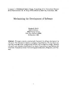
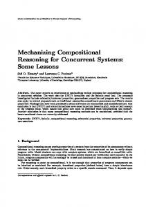
Figure 1: An in nite tree with nite branching 0

1

x0

0

1

x1 0

1

xn

and yield another such set. Similarly, List A and LList A are unary set operators over type  node set set; they can even participate in other recursive data structure de nitions.

4.1 A possible coding of lists

To understand the de nition of type  node, let us examine a simpler case, which only works for lists. The nite or in nite list [x0 ; x1 ; : : : ; xn ; : : : ] could be represented by the set of pairs

f(0; x ); (1; x ); : : : ; (n; xn ); : : : g: 0

1

Each pair consists of the position m, a natural number, paired with the label xm . To `cons' an element a to the front of this list, we must add one to all the position numbers. If succfst (m; x) = (Suc m; x) then succfst \ l increases all the position numbers in l. We may de ne the list constructors by NIL CONS

 fg

a l  f(0; a)g [ succfst \ l

S S

The function L: fNILg [ ( x l2L fCONS x lg) is clearly monotone by the properties of unions. Its lfp is the set of nite lists; its gfp includes the in nite lists too. Each list has type (  ) set, where  is the type of the list's elements.

4.2 Non-well-founded trees

In the representation above, the position of a list element is a natural number. To handle trees, let the position of a tree node be a list of natural numbers, giving the path from the root to that node. For example, the in nite tree of Figure 1 could be represented by the set of pairs

f([0]; x ); ([1; 0]; x ); : : : ; ([1| ; :{z: : ; 1}; 0]; xn ); : : : g: 0

1

n

The list [1; 1; 0] gives the position of node x2 in the tree.

4 INFINITE TREES IN HOL

10

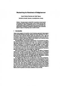
Figure 2: An in nite tree with in nite branching x0 0

1

x1 0

x1

1

x2 x 2

n

n

0

x2

x1

1 n

x 2 x2

x2

0

1

n

x2 x 2 x 2

The labelled nodes determine the tree's structure. A tree that has no labelled nodes is represented by the empty set and is indistinguishable from the empty tree. Each label de nes the corresponding position. Moreover, it implies the existence of all its ancestor nodes. With this representation, unlabelled branch nodes exist only because of the labelled leaf nodes underneath them. We can even represent trees with in nite branching. The tree of Figure 2 is the in nite set of labelled nodes of the form ([k0 ; k1 ; : : : ; kn?1 ]; xn ) for n  0 and ki :: nat. The de nitions discussed below do not exploit the representation in its full generality. Branching is nite | binary, in fact | but the depth may be in nite.

4.3 The formal de nition of type  node

A node is essentially a list paired with a label. We could represent lists as described above, but this would immediately be superseded by the resulting representation of trees, a duplication of eort. Luckily, we require only lists of natural numbers. We could encode them by Godel numbers of the form 2k0 3k1


, but they are more simply represented by functions of type nat ) nat. Let the list [k0 ; : : : ; kn?1 ] denote some function f such that (

ki if 0  i < n; if i = n. Note that f i could be anything for i > n. The constant function i:0 represents the empty list. To `cons' an element a to the front of the list f , we use Push a f , which f i=

Suc

0

is de ned by cases on its third argument:

) Suc a j Suc j ) f j Each node is represented by a pair f x, where f :: nat ) nat stands for a list Push

a f i  case i of 0

and x ::  + nat is a label. The disjoint sum type allows a label to contain either an element of type  or a natural number; some constructions below require natural numbers in trees. To prove that equality is a gfp, we must impose a niteness restriction on f . The take-lemma, which says that two lazy lists are equal if all their corresponding

4 INFINITE TREES IN HOL

11

nite initial segments are equal [5], is a standard reasoning method in lazy functional programming. The take-lemma is valid because a lazy list is nothing more than the set of its nite parts. We may similarly prove that two in nite data structures are equal, if we ensure that a tree cannot contain a node at an in nite depth. The restriction is only necessary because lists of natural numbers are represented by functions. The set of all nodes is therefore de ned as follows: Node  fp j 9f x n (p = (f; x) ^ f n = 0)g (2) The second conjunct ensures that the position list is nite: f n = 0 for some n. No other conditions need to be imposed upon nodes or node sets; the xedpoint operators exclude the undesirable elements. Since Node has a complex type, namely ((nat ) nat)  ( + nat)) set; let us de ne  node to be the type of nodes taking labels from . As described in x2.5, the subtype declaration yields abstraction and representation functions: Abs Node :: ((nat ) nat)  ( + nat)) set )  node Rep Node ::  node ) ((nat ) nat)  ( + nat)) set

4.4 The binary tree constructors

Possibly in nite binary trees represent all data structures in this theory. Binary trees are sets of nodes. The simplest binary tree, Atom a, consists of a label alone. If M and N are binary trees, then M
N is the tree consisting of the two branches M and N . Thus there are two primitive tree constructors: Atom ::  + nat )  node set (
) :: [ node set;  node set] )  node set Writing [] for i:0, we could de ne these constructors semi-formally as follows: Atom a  f([]; a)g M
N  f(Push 0 f; x)g(f;x)2M [ f(Push 1 f; x)g(f;x)2N These have the expected properties for in nite binary trees. The constructors are injective. We can recover a from Atom a; we can recover M and N from M
N by stripping the initial 0 or 1. We always have Atom a 6= M
N because Atom a contains [] as a position while M
N does not. Trees need not be WF; for example, there are in nite trees such that M = M
M . For the sake of readability, de nitions below will analyse their arguments using pattern matching instead Rep Node. Let us also abbreviate (Suc 0) as 1. The formal de nitions of Atom and (
) are cumbersome, but still readable enough: Push Node k (Abs Node(f; a))  Abs Node(Push k f; a) Atom a  fAbs Node (i:0; a)g M
N  Push Node 0 \ M [ Push Node 1 \ N

4 INFINITE TREES IN HOL

12

Now Push Node k takes the node represented by (f; a) to the one represented by (Push k f; a). Finally, the image Push Node 0 \ M applies this operation upon every node in M .

4.5 Products and sums for binary trees

One objective of this theory is to justify xedpoint de nitions of the data structures, such as List

A  lfp(Z: fNILg  (A Z ));

where is some form of Cartesian product and  is some form of disjoint sum. We cannot found these upon the usual HOL ordered pairs and injections. In both (x; y) and Inl x, the type of the result is more complex than that of the arguments; the lfp call would be ill-typed. Therefore we must nd alternative de nitions of and . Since (
) is injective, we may use it as an ordered pairing operation and de ne the product by [

[

A B  x2A y2B fx
yg Now A, B and A B all have the same type, namely  node set set. Disjoint sums are typically coded in set theory by

A + B  f(0; x)gx2A [ f(1; y)gy2B : In the present setting, this requires distinct trees to play the roles of 0 and 1. Perhaps we could nd two distinct sets of nodes, such as the empty set and the universal set, but this would complicate matters below.3 Precisely to avoid such complications, natural numbers are always allowed as labels | recall that Atom has type  + nat )  node set. The derived constructors

 )  node set Numb :: nat )  node set Leaf ::

are de ned by

a  Atom(Inl a) Numb k  Atom(Inr k ) Leaf

We may now de ne disjoint sums in the traditional manner:

M  Numb 0
M N  Numb 1
N A  B  (In0 \ A) [ (In1 \ B ) Both injections have type  node set )  node set, while A, B and A  B all have type  node set set. Since the latter type is also closed under and contains copies of In0

In1

3

The equation

fg
fg

=

fg

would frustrate the development of WF trees.

5 WELL-FOUNDED DATA STRUCTURES

13

 and nat, it has enough structure to contain virtually every sort of nitely branching

tree. Note that  and are monotonic, by the monotonicity of unions and images. The eliminators for and  are analogous to those for the product and sum types, namely split and sum case. They are de ned in the normal manner, using descriptions, and satisfy the corresponding equations: Split c (M
N ) = c M N Case c d (In0 M ) = c M Case c d (In1 N ) = d N

5 Well-founded data structures In other work [26], I have investigated the formalization of recursive data structures in Zermelo-Frnkel (ZF) set theory. It is a general approach, allowing mutual recursion; moreover, recursive set constructions may take part in new recursive de nitions, as in term A = A  list(term A). It has been mechanized within an Isabelle implementation of ZF set theory, just as the present work has been mechanized within an Isabelle implementation of HOL. It even supports non-WF data structures, using a variant form of pairing [27]. The Isabelle/HOL theory handles both WF and non-WF data structures. The WF ones are similar to those investigated in ZF, so let us dispense with them quickly.

5.1 Finite lists

We can now de ne the operator List to be the least solution to the recursion equation A = fNILg (A List A). The Knaster-Tarski Theorem applies because  and

are monotonic. We can even prove that List is a monotonic operator over type  node set set, justifying de nitions such as Term A = A List(Term A). The formal de nition of List A uses lfp to get the least xedpoint: List Fun A  Z: fNumb 0g  (A Z ) List A  lfp(List Fun A) NIL  In0(Numb 0) CONS M N  In1(M
N ) From these we can easily derive the list introduction rules (x3.1), and various injectivity properties: CONS M N 6= NIL (CONS K M = CONS L N ) = (K = L ^ M = N ) Now we can de ne case analysis (for recursion, see the next section). The eliminator for lists is expressed using those for  and : List case c d  Case (x:c) (Split d) It satis es the expected equations: List case c d NIL = c (3) List case c d (CONS M N ) = d M N (4) List

5 WELL-FOUNDED DATA STRUCTURES

14

For readability we can use this operator via Isabelle's case syntax. Later, (x6), we shall de ne LList A, which includes in nite lists, as the greatest xedpoint of List Fun A. Our de nitions of NIL, CONS and List case will continue to work, even for the in nite lists. If N is an in nite list then CONS M N is also in nite. Since List A contains no in nite lists, we may instantiate the lfp induction rule to obtain structural induction (x3.1). By induction we may prove the properties expected of a WF data structure, such as

N 2 List A (5) CONS M N 6= N The Isabelle theory proceeds to de ne the type  list to contain those values of type  node set that belong to the set List(range(Leaf)). If x1 , x2 , : : : , xn have type  then the list [x1 ; x2 ; : : : ; xn ] is represented by CONS (Leaf x1 )(CONS (Leaf x2 )(: : : CONS (Leaf xn ) NIL : : : )): Type  list has two constructors, Nil ::  list and Cons :: [;  list] )  list, and the usual induction rule, recursion operator, etc. This type de nition (x2.5) is the nal stage in making lists convenient to use; the details are routine and omitted.

5.2 A space for well-founded types

Lisp's symbolic expressions are built up from identi ers and numbers by pairing. Formalizing S-expressions in HOL further demonstrates the Isabelle theory. More importantly, it leads to a uniform treatment of recursive functions for virtually all nitely branching WF data structures. An essential feature of S-expressions is that they are nite. Therefore, let us de ne them using lfp: Sexp

 lfp(Z: range(Leaf) [ range(Numb) [ (Z Z ))

(6)

Observe how range expresses the sets of all Leaf a and Numb k constructions. We can develop Sexp in the same manner as List A, deriving an induction rule, a case analysis operator, etc. But Sexp is a rather special subset of our universe, itself suitable for de ning recursive data structures. It contains all constructions of the form Leaf a, Numb k and M
N , and therefore also In0 M and In1 N . Thus it is closed under and . De ned by lfp, all the constructions in it are nite. Now Sexp is not necessarily large enough to contain List A for arbitrary A, since A might contain in nite constructions. But Sexp is closed under List: we can easily prove List(Sexp)  Sexp, expressing that lists of nite constructions are themselves nite constructions. Similarly, Sexp is closed under many other nite data structures. Recursion on Sexp gives us recursion on all these WF data structures. Isabelle's HOL theory contains a derivation of WF recursion. This justi es de ning any function whose recursive calls decrease its argument under some WF relation. The immediate subexpression relation on Sexp is the set of pairs () 

[

[ f(M; M
N ); (N; M
N )g: M 2Sexp N 2Sexp

6 LAZY LISTS AND COINDUCTION

15

Structural induction on Sexp proves that this relation is WF. The transitive closure of a relation can be de ned using lfp, and can be proved to preserve wellfoundedness [26]. So M + N expresses that M is a subexpression of N . WF recursion justi es any function on S-expressions whose recursive calls take subexpressions of the original argument. Let us apply this to lists. Recall that CONS M N  In1(M
N )  Numb 1
(M
N ): A sublist is therefore a subexpression. Structural recursion on lists is an instance of WF recursion. Suppose f is de ned by f M  wfrec (+ ) M (M g: case M of NIL )c j CONS x y ) d x y (g y)) We immediately obtain f NIL = c. The fact N + CONS M N justi es the recursion equation

M 2 Sexp N 2 Sexp f (CONS M N ) = d M N (f N ):

Most familiar list functions | append, reverse, map | have obvious de nitions by structural recursion. But the theory does not insist upon structural recursion; it can express functions such as quicksort in their natural form, using WF recursion in its full generality. De nition (6) is not the only possible way of characterizing the set of nite constructions. We could instead formalize the nite powerset operator using lfp [26]. The set of all nite, non-empty sets of nodes would be larger than Sexp while satisfying the same key closure properties. De ning a suitable WF relation on this set might be tedious. The Isabelle/HOL theory of WF data structures is quite general, at least for nite branching. Non-WF data structures pose greater challenges.

6 Lazy lists and coinduction De ning the set of lists as a greatest instead of a least xedpoint admits in nite as well as nite lists. We can then model computation and equality, realizing to some extent the theory of lists in lazy functional languages [5]. However, our \lazy lists" have no inbuilt operational semantics; after all, HOL can express non-computable functions. The set of lazy lists is de ned by LList A  gfp(List Fun A); recall that List Fun and the list operations NIL, CONS and List case were de ned in x5.1. The xedpoint property yields introduction rules for LList A: NIL

2 LList A

M 2 A N 2 LList A CONS M N 2 LList A

These may resemble their nite list counterparts (x3.1), but they dier signi cantly, for CONS is well-behaved even when applied to an in nite list. In particular, the List case equation (4) works for everything of the form CONS M N .

6 LAZY LISTS AND COINDUCTION

16

Since LList A is a greatest xedpoint, it does not have a structural induction principle. Well-foundedness properties such as the list theorem (5) have no counterparts for LList A. We can construct a counterexample and prove that it belongs to LList A by coinduction. The weak coinduction rule for LList A performs type checking for in nite lists:

M 2 X X  List Fun A X M 2 LList A

(7)

M 2 X X  List Fun A X [ LList A M 2 LList A

(8)

The strong coinduction rule, as described in x3.2, implicitly includes LList A:

6.1 An in nite list

One non-WF list is the in nite list of M s: Lconst

M = CONS M (Lconst M )

(9)

Corecursion, a general method for de ning in nite lists, is discussed below. For now, let us construct Lconst M explicitly as a xedpoint: Lconst

M  lfp(Z: CONS M Z )

The Knaster-Tarski Theorem applies because lists are sets of nodes and CONS is monotonic in both arguments. (Recall from x4.4 that (
) is de ned in terms of the monotonic operations union and image.) I have used lfp but gfp would work just as well | we need only the xedpoint property (9). We cannot prove that Lconst M is a lazy list by the introduction rules alone. The coinduction rule (7) proves Lconst M 2 LListfM g if we can nd a set X containing Lconst M and included in List Fun fM g X . A suitable X is fLconst M g. Obviously Lconst M 2 fLconst M g. We must also show

fLconst M g  List Fun fM g fLconst M g: The xedpoint property (9) transforms this to

fCONS M (Lconst M )g  List Fun fM g fLconst M g; which is obvious by the de nitions of CONS and List Fun. Deriving introduction rules for List Fun allows shorter machine proofs:

2 List Fun A X M 2A N 2X CONS M N 2 List Fun A X NIL

(10) (11)

6 LAZY LISTS AND COINDUCTION

17

6.2 Equality of lazy lists; the take-lemma

Because HOL lazy lists are sets of nodes, the equality relation on LList A is an instance of ordinary set equality. By investigating this relation further, we obtain nice, coinductive methods for proving that two lazy lists are equal. Let take k l return l's rst k elements as a nite list. Bird and Wadler [5] use the take-lemma to prove equality of lazy lists l1 and l2 : 8k take k l1 = take k l2 l1 = l2 It embodies a continuity principle shared by our HOL formalization. The de nition (2) of nodes (in x4.3) requires each node to have a nite depth. A node contains a pair (f; x), where x is the label and f codes the position. Our de nition ensures f k = 0 for some k, which is the depth of the node. We can formalize the depth directly, using the least number principle and pattern matching:

k: k  k: k ^ (8j (j < k ! :j )) ndepth (Abs Node(f; x))  LEAST k: f k = 0 LEAST

Our generalization of take, called ntrunc, applies to all data structures, not just lists. It returns the set of all nodes having less than a given depth: ntrunc

k N  fnd j nd 2 N ^ ndepth nd < kg

Elementary reasoning derives results describing ntrunc's eect upon various constructions:

M = fg k) (Leaf a) = Leaf a ntrunc (Suc k ) (Numb a) = Numb a ntrunc (Suc k ) (M
N ) = ntrunc k M
ntrunc k N Since In0 M  Numb 0
M we obtain ntrunc 0

ntrunc (Suc

M ) = fg k)) (In0 M ) = In0(ntrunc (Suc k) M )

ntrunc 1 (In0

ntrunc (Suc(Suc

and similarly for In1. Our generalization of take enjoys a generalization of the take-lemma: Lemma 1 If ntrunc k M = ntrunc k N for all k then M = N . This obvious fact is a key result. It gives us a method for proving the equality of any constructions M and N . We could apply this \ntrunc-lemma" directly, but instead we shall package it into a form suitable for coinduction.

6 LAZY LISTS AND COINDUCTION

18

6.3 Diagonal set operators

In order to prove list equations by coinduction, we must demonstrate that the equality relation is the greatest xedpoint of some monotone operator. To this end, we de ne diagonal set operators for and . A diagonal set has the form f(x; x)gx2A , internalizing the equality relation on A. A binary relation on sets of nodes has type ( node set   node set) set. The operators D and D combine two such relations to yield a third. The operator diag, of type  set ) (  ) set, constructs arbitrary diagonal sets. [

A  x2A f(x; x)g [ [ r D s  (x;x )2r (y;y )2s f(x
y; x0
y0 )g

diag

r D s 

0

[

0

0 2r f(In0 x; In0 x )g [

x;x )

(

0

[

y;y )2s

(

0

f(In1 y; In1 y0 )g

These enjoy readable introduction rules. For D we have (M; M 0 ) 2 r (N; N 0 ) 2 s (M
N; M 0
N 0 ) 2 r D s while for D we have the pair of rules (M; M 0 ) 2 r (N; N 0 ) 2 s (In0 M; In0 M 0 ) 2 r D s (In1 N; In1 N 0 ) 2 r D s The idea is that D and D build relations in the same manner as and  build sets. Since fst \ r is the rst projection of the relation r, we can summarize the idea by three obvious equations:

A=A fst \ (r D s) = (fst \ r) (fst \ s) fst \ (r D s) = (fst \ r)  (fst \ s) fst \ diag

Category theorists may note that and  are functors on a category of sets where the morphisms are binary relations; in this category, D and D give the functors' eects on the morphisms. Next, we shall do the same thing to the functor LList.

6.4 Equality of lazy lists as a gfp

Just as D and D extend and  to act upon relations, let LListD extend LList. Thanks to our new operators, the de nition is simple and resembles that of LList:

r  Z: diagfNumb 0g D (r D Z ) LListD r  gfp(LListD Fun r)

LListD Fun

The theorem that list equality is a gfp can now be stated as a succinct equation between relations: LListD(diag A) = diag(LList A). Here diag(LList A) is the equality relation on LList A, while LListD(diag A) is the gfp of LListD Fun(diag A). Proving this requires another lemma about ntrunc.

6 LAZY LISTS AND COINDUCTION

19

Lemma 2 8M N [(M; N ) 2 LListD(diag A) ! ntrunc k M = ntrunc k N ]. Proof By complete induction on k, we may assume the formula above after replacing k by any smaller natural number j . By the xedpoint property LListD(diag A) = diagfNumb 0g D (r D LListD(diag A)); if (M; N ) 2 LListD(diag A) then there are two cases. If M = N = In0(Numb 0) = NIL then ntrunc k M = ntrunc k N is trivial. Otherwise M = CONS x M 0 and N = CONS x N 0 , where (M 0 ; N 0 ) 2 LListD(diag A). Recall the de nition CONS x y  In1(x
y ) and the properties of ntrunc (x6.2); we obtain (

k (CONS x y) = fg

if k < 2, and CONS (ntrunc j x) (ntrunc j y ) if k = Suc(Suc j ). If k = Suc(Suc j ) then ntrunc k M = ntrunc k N reduces to an instance of the induction hypothesis, ntrunc j M 0 = ntrunc j N 0 . Now we can prove that equation. Proposition 3 LListD(diag A) = diag(LList A). Proof Combining Lemmas 1 and 2 yields half of our desired result, LListD(diag A)  diag(LList A). This is the more important half: it lets us show M = N by showing (M; N ) 2 LListD(diag A), which can be done using coinduction. The opposite inclusion, diag(LList A)  LListD(diag A), follows by showing that diag(LList A) is a xedpoint of LListD Fun(diag A), since LListD(diag A) is the greatest xedpoint. This argument is an example of coinduction. ntrunc

6.5 Proving lazy list equality by coinduction

The weak coinduction rule for list equality yields M = N provided (M; N ) 2 r where r is a suitable bisimulation between lazy lists: (M; N ) 2 r r  LListD Fun(diag A)r (12) M =N

Coinduction has many variant forms (x3.2). Strong coinduction includes the equality relation implicitly in every bisimulation: (M; N ) 2 r r  LListD Fun(diag A)r [ diag(LList A) (13) M =N Expanding the de nitions of NIL, CONS and LListD Fun creates unwieldy formulae. The Isabelle theory derives two rules to avoid this, resembling the List Fun rules (10) and (11): (NIL; NIL) 2 LListD Fun(diag A)r (14)

x 2 A (M; N ) 2 r (CONS x M; CONS x N ) 2 LListD Fun(diag A)r

(15)

7 LAZY LISTS AND CORECURSION

20

7 Lazy lists and corecursion We have de ned the in nite list Lconst M = [M; M; : : : ] using a xedpoint. The construction clearly generalizes to other repetitive lists such as [M; N; M; N; : : : ]. But how can we de ne in nite lists such as [1; 2; 3; : : : ]? And how can we de ne the usual list operations, like append and map? Structural recursive de nitions would work for elements of List A but not for the in nite lists in LList A. Corecursion is a dual form of structural recursion. Recursion de nes functions that consume lists, while corecursion de nes functions that create lists. Corecursion originated in the category theoretic notion of nal coalgebra; Mendler [19] and Geuvers [12], among others, have investigated it in type theories. This paper does not attempt to treat corecursion categorically. And instead of describing the general case in all its complexity, it simply treats a key example: lazy lists. Let us begin with motivation and examples.

7.1 Introduction to corecursion

Corecursion de nes a lazy list in terms of some seed value a ::  and a function f ::  ) unit + ( node set  ). Recall from x2.3 that unit is the nullary product type, whose sole value is (), while  and + are the product and sum type operators. Thus LList corec has type [;  ) unit + ( node set  )] ) node set: It must satisfy ( NIL if f a = Inl (); LList corec a f = CONS x (LList corec b f ) if f a = Inr (x; b). The idea should be clear: f takes the seed a and either returns Inl (), to end the list here, or returns Inr (x; b), to continue the list with next element x and seed b. By keeping the seed forever M and always returning it as the next element, corecursion can express Lconst M : Lconst M  LList corec M (N:Inr (N; N )) Consider the functional Lmap, which applies a function to every element of a list: Lmap g [x0 ; x1 ; : : : ; xn ; : : : ] = [g x0 ; g x1 ; : : : ; g xn ; : : : ] The usual recursion equations are Lmap g NIL = NIL (16) Lmap g (CONS M N ) = CONS (g M ) (Lmap g N ): (17) Corecursion handles these easily. To compute Lmap g M , take M as the seed. If M = NIL then end the result list; if M = CONS x M 0 then continue the result list with next element g x and seed M 0 . The formal de nition uses List case to inspect M : Lmap g M  LList corec M (M: case M of NIL ) Inl () j CONS x M 0 ) Inr (g x; M 0 )) This de nition of map has little in common with the standard recursive one. Append comes out stranger still, and other standard functions seem to be lost altogether.

7 LAZY LISTS AND CORECURSION

21

7.2 Harder cases for corecursion

With corecursion, the case analysis is driven by the output list, rather than the input list. The append function highlights this peculiarity. The usual recursion equations for append perform case analysis on the rst argument:

N =N Lappend (CONS M1 M2 ) N = CONS M1 (Lappend M2 N ) Lappend NIL

But a NIL input does not guarantee a NIL output, as it did for Lmap; consider Lappend NIL (CONS

M N ) = CONS M N:

The correct equations for corecursion involve both arguments: Lappend NIL NIL = NIL

(18) (19) (20)

N1 N2 ) = CONS N1 (Lappend NIL N2 ) Lappend (CONS M1 M2 ) N = CONS M1 (Lappend M2 N )

Lappend NIL (CONS

The second line above forces Lappend NIL N to continue executing until it has made a copy of N . This looks inecient. In the context of the polymorphic -calculus, Geuvers [12] discusses stronger forms of corecursion that allow the seed to return an entire list at once. But my HOL theory has no operational signi cance; eciency is meaningless; we may as well keep corecursion simple.4 The seed for Lappend M N is the pair (M; N ). The corecursive de nition performs case analysis on both lists:  If M = NIL then it looks at N : { If N = NIL then end the result list. { If N = CONS N1 N2 then continue the result list with next element N1 and seed (NIL; N2 ).  If M = CONS M1 M2 then continue the result list with next element M1 and seed (M2 ; N ). We can formalize this using LList corec. De ne f by case analysis:

f  (M; N ): case M

of

) (case N of

NIL

NIL ) Inl () j CONS N N ) Inr (N ; (NIL; N )))

j CONS M M ) Inr (M ; (M ; N )) Then put Lappend M N  LList corec (M; N ) f . 1

2

1

1

2

1

2

2

4 This relates to diculties with formalizing (co)inductive de nitions in type theory. Under some formalizations, the constructors of coinductive types are complicated and inecient | and dually, so are the destructors of inductive types. This does not occur in my HOL treatment: constructors and destructors are directly available from the xedpoint equations. Thus we must not push the analogy with type theory too far.

7 LAZY LISTS AND CORECURSION

22

Concatenation. Now let us try to de ne a function to atten a list of lists according to the following recursion equations:

Lflat NIL = NIL

Lflat(CONS

M N ) = Lappend M (Lflat N )

(21) (22)

Since corecursion is driven by the output, we need to know when a CONS is produced. We can re ne equation (22) by further case analysis:

N ) = Lflat N Lflat(CONS (CONS M1 M2 ) N ) = CONS M1 (Lflat(CONS M2 N )) Unfortunately, the outcome of CONS NIL N is still undecided; it could be NIL or CONS. Lflat(CONS NIL

Given the argument Lconst NIL | an in nite list of NILs | Lflat should run forever. There is no eective way to check whether an in nite list contains a non-NIL element. I do not know of any natural formalization of Lflat. Since HOL can formalize non-computable functions, we can force Lflat (Lconst NIL) = NIL using a description. Such a de nition would be of little relevance to computer science. Really Lflat (Lconst NIL) should be unde ned, but HOL does not admit partial functions. The lter functional, which removes from a list all elements that fail to satisfy a given predicate, poses similar problems. If no list elements satisfy the predicate, then the result is logically NIL, but there is no eective way to reach this result. Leclerc and Paulin-Mohring [17] discuss approaches to this problem in the context of the Coq system.

7.3 Deriving corecursion

The characteristic equation for corecursion can be stated using case analysis and pattern matching:

a f = case f a of (23) Inl u ) NIL j Inr(x; b) ) CONS x (LList corec b f ) To realize this equation, recall that an element of LList A is a set of nodes, each of LList corec

nite depth. A primitive recursive function can approximate the corecursion operator for nodes up to some given depth k:

a f = fg lcorf (Suc k ) a f = case f a of Inl u ) NIL j Inr(x; b) ) CONS x (lcorf k b f ) lcorf 0

Now we can easily de ne corecursion: LList corec

[

a f  k lcorf k a f

Equation (23) can then be proved as two separate inclusions, with simple reasoning about unions and (in one direction) induction on k.

8 EXAMPLES OF COINDUCTION AND CORECURSION

23

The careful reader may have noticed that lcorf k a f is not strictly primitive recursive, because the parameter a varies in the recursive calls. To be completely formal, we must de ne a function over a using higher-order primitive recursion. In the Isabelle theory, lcorf k a f becomes LList corec fun k f a. It can be de ned by primitive recursion:

f = a: fg LList corec fun (Suc k ) f = a: case f a of Inl u ) NIL j Inr(x; b) ) CONS x (LList corec fun k f b) LList corec fun 0

Obscure as this may look, it trivially implies the equations for lcorf given above.

8 Examples of coinduction and corecursion This section demonstrates de ning functions by corecursion and verifying their equational and typing properties by coinduction. All these proofs have been checked by machine.

8.1 A type-checking rule for LList corec

One advantage of LList corec over ad-hoc de nitions is that the result is certain to be a lazy list. To express this well-typing property in the simplest possible form, let U ::  node set set abbreviate the universal set of constructions: U  fx j Trueg. We can now state a typing result: Example 4 LList corec a f 2 LList U .

Proof Apply the weak coinduction rule (7) to the set V  range(x: LList corec x f ): We must show V  List Fun U V , which reduces to LList corec a f 2 List Fun U V: There are two cases. We simplify each case using equation (23):  If f a = Inl (), it reduces to NIL 2 List Fun U V , which holds by Rule (10).  If f a = Inr (x; b), it reduces to

x (LList corec b f ) 2 List Fun U V: This holds by Rule (11) because x 2 U and LList corec b f 2 V . CONS

This result, referring to the universal set, may seem weak compared with our previous well-typing result, Lconst M 2 LListfM g, from x6.1. It is dicult to bound the set of possible values for x for the case f a = Inr (x; b). Sharper results can be obtained by performing separate coinduction proofs for each function de ned by corecursion.

8 EXAMPLES OF COINDUCTION AND CORECURSION

24

8.2 The uniqueness of corecursive functions

Equation (23) characterizes LList corec uniquely; the proof is a typical example of proving an equation by coinduction. Let us de ne an abbreviation for the corecursion property: is corec

f h  8u [h u = case f u of

Inl v ) NIL j Inr(x; b) ) CONS x (h b)]

Existence, namely is corec f (x: LList corec x f ), is immediate by equation (23). Let us now prove uniqueness.

Proposition 5 If is corec f h and is corec f h then h = h . Proof By extensionality it suces to prove h u = h u for all u. Now consider the bisimulation f(h u; h u)gu , formalized in HOL by r  range(u: (h u; h u)): Apply the coinduction rule (12), with r as above and putting A  U , the universal set. We must show r  LListD Fun(diag U )r; since elements of r have the form 1

2

1

1

1

2

2

2

1

2

(h1 u; h2 u) for arbitrary u, it suces to show

(h1 u; h2 u) 2 LListD Fun(diag U )r: There are two cases, determined by f (u). In each, we apply the corecursion properties of h1 and h2 :  If f u = Inl (), it reduces to (NIL; NIL) 2 LListD Fun(diag U )r, which holds by Rule (14).  If f u = Inr (x; b), it reduces to (CONS x (h1 b); CONS x (h2 b)) 2 LListD Fun(diag U )r: This holds by Rule (15) because x 2 U and (h1 b; h2 b) 2 r. Note the similarity between this coinduction proof and the previous one, even though the former proves set membership while the latter proves an equation. The role of r in this equality proof is reminiscent of process equivalence proofs in CCS [20], where the bisimulation associates corresponding states of two processes. The equality can also be proved using Lemma 1 directly, by complete induction on k; the proof is considerably more complex.

8.3 A proof about the map functional

To demonstrate that the theory has some relevance to lazy functional programming, this section proves a simple result: that map distributes over composition.

Example 6 If M 2 LList A then Lmap (f  g) M = Lmap f (Lmap g M ).

8 EXAMPLES OF COINDUCTION AND CORECURSION

25

Proof The bisimulation f(Lmap (f  g) u; Lmap f (Lmap g u))gu2LList A may be formalized using the image operator: r  (u: (Lmap (f  g) u; Lmap f (Lmap g u))) \ LList A As in the previous coinduction proof, apply Rule (12). The key is to show (Lmap (f  g) u; Lmap f (Lmap g u)) 2 LListD Fun(diag U )r for arbitrary u 2 LList A. There are again two cases, this time depending on the form of u. We simplify each case using the recursion equations for Lmap, which follow from its corecursive de nition (x7.1).  If u = NIL, the goal reduces to (NIL; NIL) 2 LListD Fun(diag U )r, which holds by Rule (14).  If u = CONS M 0 N , it reduces to (CONS (f (g M 0)) (Lmap (f  g) N ); CONS (f (g M 0 )) (Lmap f (Lmap g N ))) 2 LListD Fun(diag U )r: This holds by Rule (15) because f (g M 0 ) 2 U and (Lmap (f  g) N; Lmap f (Lmap g N )) 2 r: The coinductive argument bears little resemblance to the usual proof in the Logic for Computable Functions (LCF) [22, page 283]. On the other hand, all these coinductive proofs have a monotonous regularity. A similar argument proves Lmap (x:x) M = M .

8.4 Proofs about the list of iterates Consider the function Iterates de ned by

f M  LList corec M (M: Inr (M; f M )): A generalization of Lconst, it constructs the in nite list [M; f M; : : : ; f n M; : : : ] by Iterates

the recursion equation

Iterates

f M = CONS M (Iterates f (f M )):

The equation Lmap

f (Iterates f M ) = Iterates f (f M )

(24)

has a straightforward coinductive proof, using the bisimulation f(Lmap f (Iterates f u); Iterates f (f u))gu2LList A : Combining the previous two equations yields a new recursion equation, involving Lmap: Iterates f M = CONS M (Lmap f (Iterates f M )) Harder is to show that this equation uniquely characterizes Iterates f .

8 EXAMPLES OF COINDUCTION AND CORECURSION

26

Example 7 If h x = CONS x (Lmap f (h x)) for all x then h = Iterates f . Proof The bisimulation for this proof is unusually complex. Let f n stand for the

function that applies f to its argument n times. Since Lmap is a curried function, the function (Lmap f )n applies Lmap f to a given list n times. The bisimulation has two index variables:

r  f((Lmap f )n (h u); (Lmap f )n (Iterates f u))gu2LList U; n0 Recall that U stands for the universal set of the appropriate type. Then note two facts, both easily justi ed by induction on n: (Lmap f )n (CONS b M ) = CONS (f n b) ((Lmap f )n M ) f n (f x) = f Suc n x

(25) (26)

By extensionality it suces to prove h u = Iterates f u for all u. Again we apply the weak coinduction rule (12), with the bisimulation r shown above. The key step in verifying the bisimulation is to show ((Lmap f )n (h u); (Lmap f )n (Iterates f u)) 2 LListD Fun(diag U )r for arbitrary n  0 and u 2 LList U . By the recursion equations for h and Iterates, the pair expands to ((Lmap f )n (CONS u (Lmap f (h u))); (Lmap f )n (CONS u (Iterates f (f u)))) and now two applications of equation (25) yield (CONS (f n u) ((Lmap f )n (Lmap f (h u))); CONS (f n u) ((Lmap f )n (Iterates f (f u)))) Applying Rule (15) to show membership in LListD Fun(diag U )r, we are left with the subgoal ((Lmap f )n (Lmap f (h u)); (Lmap f )n (Iterates f (f u))) 2 r: By equations (24) and (26) we obtain (Lmap f Suc n (h u); Lmap f Suc n (Iterates f u)) 2 r; which is obviously true, by the de nition of r. Pitts [28] describes a similar coinduction proof in domain theory. The function does not lend itself to reasoning by structural induction, but is amenable to Scott's xedpoint induction; I proved equation (24) in the Logic for Computable Functions (LCF) [22, page 286].

Iterates

8 EXAMPLES OF COINDUCTION AND CORECURSION

27

8.5 Reasoning about the append function

Many accounts of structural induction start with proofs about append. But append is not an easy example for coinduction. Remember that the corecursive de nition does not give us the usual pair of equations, but rather the three equations (18){(20). Proofs by the weak coinduction rule (12) typically require the same three-way case analysis. Consider proving that map distributes over append: Example 8 If M 2 LList A and N 2 LList A then Lmap

f (Lappend M N ) = Lappend (Lmap f M ) (Lmap f N ):

Proof Applying the weak coinduction rule with the bisimulation f(Lmap f (Lappend u v); Lappend (Lmap f u) (Lmap f v))gu2LList A;v2LList A ; we must show (Lmap f (Lappend u v); Lappend (Lmap f u) (Lmap f v )) 2

LListD Fun(diag

U )r:

Considering the form of u and v, there are three cases:  If u = v = NIL, the pair reduces by equations (16) and (18) to (NIL; NIL), and Rule (14) solves the goal.  If u = NIL and v = CONS N1 N2 , the pair reduces by equations (16), (17) and (19) to (CONS (f N1 ) (Lmap f (Lappend NIL N2 )); CONS (f N1 ) (Lappend NIL (Lmap f N2 ))): Using equation (16) to replace the second NIL by Lmap f NIL restores the form of the bisimulation, so that Rule (15) can conclude this case.  If u = CONS M1 M2 , the pair reduces by equations (17) and (20) to (CONS (f M1 ) (Lmap f (Lappend M2 v)); CONS (f M1 ) (Lappend (Lmap f M2 ) (Lmap f v ))): Now Rule (15) solves the goal, proving the distributive law. Two easy theorems state that NIL is the identity element for Lappend. For M 2 A we have

LList

Lappend NIL

M = M and

Lappend

M NIL = M

(27)

Both proofs have only two cases because M is the only variable. The strong coinduction rule (13) can prove the distributive law with only two cases. Recall from x6.5 that the latter rule implicitly includes the equality relation in the bisimulation; if we can reduce the pair to the form (a; a), then we are done. The

8 EXAMPLES OF COINDUCTION AND CORECURSION

28

simpler proof applies the strong coinduction rule (13), using the same bisimulation as before. Now we must show (Lmap f (Lappend u v); Lappend (Lmap f u) (Lmap f v )) 2

U )r [ diag(LList U ): There are two cases, considering the form of u. If u = CONS M1 M2 then reason exactly as in the previous proof. If u = NIL, the goal reduces by (16) and (27) to (Lmap f v; Lmap f v) 2

LListD Fun(diag

LListD Fun(diag

U )r [ diag(LList U ):

The pair belongs to diag(LList U ) because Lmap f v 2 LList U .

Typing rules. Most of our coinduction examples prove equations. But coinduction can also prove typing facts such as Lappend M N 2 LList A. Again, strong coinduc-

tion works better for Lappend than weak coinduction. The weak rule (7), requires case analysis on both arguments of Lappend; three cases must be considered. The strong rule (8) requires only case analysis on the rst argument. The two proofs are closely analogous to those of the distributive law.

Associativity. A classic example of structural induction is the associativity of ap-

pend:

Lappend (Lappend

M1 M2 ) M3 = Lappend M1 (Lappend M2 M3)

With weak coinduction, the proof is no longer trivial; it involves a bisimulation in three variables and the proof consists of four cases: NIL-NIL-NIL, NIL-NIL-CONS, NILCONS, and CONS. Strong coinduction with the bisimulation

f(Lappend (Lappend u M ) M ; Lappend u (Lappend M M ))gu2LList A 2

3

2

3

accomplishes the proof easily. There are only two cases. If u = CONS M M 0 then the pair reduces to (CONS M (Lappend (Lappend M 0 M2 ) M3 ); CONS M (Lappend M 0 (Lappend M2 M3 ))) and Rule (15) applies as usual. If u = NIL then both components collapse to Lappend M2 M3 , and the pair belongs to the diagonal set.

8.6 A comparison with LCF

Scott's Logic for Computable Functions (LCF) is ideal for reasoning about lazy data structures.5 Types denote domains and function symbols denote continuous functions. Strict and lazy recursive data types can be de ned. Domains contain the bottom

Scott's 1969 paper, which laid the foundations of domain theory, has nally been published [30]. Edinburgh LCF [15], a highly in uential system, implemented Scott's logic. Still in print is my account of a successor LCF system [22]. Isabelle provides two versions of LCF: one built upon rst-order logic, the other built upon Isabelle/HOL. 5

9 CONCLUSIONS

29

element ?, which is the denotation of a divergent computation. Objects can be partial, with components that equal ?. A function f can be partial, with f x = ? for some x. A lazy list can be partial, with its head, tail or some elements equal to ?. The relation x v y, meaning \x is less de ned or equal to y," compares partial objects. LCF's xedpoint operator expresses recursive objects, including partial functions and recursive lists. The xedpoint induction rule reasons about the unwinding of recursive objects. It subsumes the familiar structural induction rules and even generalizes them to reason about in nite objects, when the induction formula is chaincomplete. Since all formulae of the form x v y and x = y are chain-complete, LCF can prove equations about lazy lists. Can our HOL treatment of lazy lists compare with LCF's? The Isabelle theory de nes the new type  llist to contain the elements of LList(range(Leaf)), replacing the clumsy set reasoning by automatic type checking. We can still de ne lists by corecursion and prove equations by coinduction. The resulting theory of lazy lists is super cially similar to LCF's. But it lacks general recursion and cannot handle divergent computations. Leclerc and PaulinMohring's construction of the prime numbers in Coq [17] re ects these problems. Corecursion cannot express the lter functional, needed for the Sieve of Eratosthenes. A direct comparison between xedpoint induction and coinduction is dicult. The rules dier greatly in form and their area of overlap is small. Fixedpoint induction can reason about recursive programs at an abstract level, for instance to prove equivalence of partial functions. Coinduction can prove the equivalence of in nite processes. I prefer LCF for problems that can be stated entirely in domain theory. But LCF is a restrictive framework: all types must denote domains; all functions must be continuous. HOL is a general logic, free of such restrictions, and yet capable of handling a substantial part of the theory of lazy lists.

9 Conclusions This mechanized theory is a comprehensive treatment of recursive data structures in higher-order logic, generalizing Melham's theory [18]. Melham's approach is concrete: one particular tree structure represents all recursive types. My xedpoint approach is more abstract, which facilitates extensions such as mutual recursion [26] and in nite branching trees. Users may also add new monotone operators to the type de nition language. Types need not be free (such that each constructor function is injective); for example, we may de ne the set Fin A of all nite subsets of A as a least xedpoint: Fin



A  lfp Z:ffgg [

[ [  ff x g [ y g y2Z x2A

Most importantly, the theory justi es non-WF data structures. Elsa Gunter [16] has independently developed a theory of trees, using ideas similar to those of x4. Her aim is to extend Melham's package with in nite branching, rather than coinduction. What about set theory? The ordered pair (a; b) is traditionally de ned to be ffag; fa; bgg. Non-WF data structures presuppose non-WF sets, with in nite descents along the 2 relation. Such sets are normally forbidden by the Foundation Axiom, but

REFERENCES

30

the Anti-Foundation Axiom (AFA) asserts their existence. Aczel [3] has analysed and advocated this axiom; some authors, such as Milner and Tofte [21], have suggested formalizing coinductive arguments using it. But non-WF lists and trees are easily expressed in set theory without new axioms. Simply use the ideas presented above for Isabelle/HOL. A new de nition of ordered pair, based upon the old one, allows in nite descents. De ne the variant ordered pair (a; b) to be f(0; x)gx2a [ f(1; y)gy2b. This is equivalent to the disjoint sum a + b as usually de ned, but note also its similarity to M
N (see x4.4). Elsewhere [27] I have developed this approach; it handles recursive data structures in full generality, but not the models of concurrency that motivated Aczel. The proof of the main theorem is inspired by that of Lemma 2. Isabelle/ZF mechanizes this theory. The theory of coinduction requires further development. Its treatment of lazy lists is clumsy compared with LCF's. Stronger principles of coinduction and corecursion might help. Its connection with similar work in stronger type theories [12, 17] deserves investigation. Leclerc and Paulin-Mohring [17] remark that Coq can express nite and in nite data structures in a manner strongly reminiscent of the Knaster-Tarski Theorem. They proceed to consider a representation of streams that speci es the possible values of the stream member at position i, where i is a natural number. Generalizing this approach to other in nite data structures requires generalizing the notion of position, perhaps as in x4.2. Jacob Frost [11] has performed Milner and Tofte's coinduction example [21] using Isabelle/HOL and Isabelle/ZF. The most dicult task is not proving the theorem but formalizing the paper's non-WF de nitions. As of this writing, Isabelle/HOL provides no automatic means of constructing the necessary de nitions and proofs.

Acknowledgements. Jacob Frost, Sara Kalvala and the referees commented on the paper. Martin Coen helped to set up the environment for coinduction proofs. Andrew Pitts gave much advice, for example on proving that equality is a gfp. Tobias Nipkow and his colleagues have made substantial contributions to Isabelle. The research was funded by the SERC (grants GR/G53279, GR/H40570) and by the ESPRIT Basic Research Actions 3245 `Logical Frameworks' and 6453 `Types'.

References

[1] S. Abramsky. The lazy lambda calculus. In D. A. Turner, editor, Resesarch Topics in Functional Programming, pages 65{116. Addison-Wesley, 1977. [2] P. Aczel. An introduction to inductive de nitions. In J. Barwise, editor, Handbook of Mathematical Logic, pages 739{782. North-Holland, 1977. [3] P. Aczel. Non-Well-Founded Sets. CSLI, 1988. [4] P. B. Andrews, M. Bishop, S. Issar, D. Nesmith, F. Pfenning, and H. Xi. TPS: A theorem proving system for classical type theory. J. Auto. Reas., 16(1), 1996. In press. [5] R. Bird and P. Wadler. Introduction to Functional Programming. Prentice-Hall, 1988. [6] A. Church. A formulation of the simple theory of types. J. Symb. Logic, 5:56{68, 1940. [7] L. J. M. Claesen and M. J. C. Gordon, editors. Higher Order Logic Theorem Proving and Its Applications. North-Holland, 1993. [8] T. Coquand and C. Paulin. Inductively de ned types. In P. Martin-Lof and G. Mints, editors, COLOG-88: International Conference on Computer Logic, LNCS 417, pages 50{66, Tallinn, Published 1990. Estonian Academy of Sciences, Springer.

REFERENCES

31

[9] B. A. Davey and H. A. Priestley. Introduction to Lattices and Order. Cambridge Univ. Press, 1990. [10] W. M. Farmer, J. D. Guttman, and F. J. Thayer. IMPS: An interactive mathematical proof system. J. Auto. Reas., 11(2):213{248, 1993. [11] J. Frost. A case study of co-induction in Isabelle. Technical Report 359, Comp. Lab., Univ. Cambridge, Feb. 1995. [12] H. Geuvers. Inductive and coinductive types with iteration and recursion. In B. Nordstrom, K. Petersson, and G. Plotkin, editors, Types for Proofs and Programs, pages 193{217, Bastad, June 1992. informal proceedings. [13] J.-Y. Girard. Proofs and Types. Cambridge Univ. Press, 1989. Translated by Yves LaFont and Paul Taylor. [14] M. J. C. Gordon and T. F. Melham. Introduction to HOL: A Theorem Proving Environment for Higher Order Logic. Cambridge Univ. Press, 1993. [15] M. J. C. Gordon, R. Milner, and C. P. Wadsworth. Edinburgh LCF: A Mechanised Logic of Computation. Springer, 1979. LNCS 78. [16] E. L. Gunter. A broader class of trees for recursive type de nitions for hol. In J. Joyce and C. Seger, editors, Higher Order Logic Theorem Proving and Its Applications: HUG '93, LNCS 780, pages 141{154. Springer, Published 1994. [17] F. Leclerc and C. Paulin-Mohring. Programming with streams in Coq. a case study: the sieve of Eratosthenes. In H. Barendregt and T. Nipkow, editors, Types for Proofs and Programs: International Workshop TYPES '93, LNCS 806, pages 191{212. Springer, 1993. [18] T. F. Melham. Automating recursive type de nitions in higher order logic. In G. Birtwistle and P. A. Subrahmanyam, editors, Current Trends in Hardware Veri cation and Automated Theorem Proving, pages 341{386. Springer, 1989. [19] N. P. Mendler. Recursive types and type constraints in second-order lambda calculus. In Second Annual Symposium on Logic in Computer Science, pages 30{36. ieee Comp. Soc. Press, 1987. [20] R. Milner. Communication and Concurrency. Prentice-Hall, 1989. [21] R. Milner and M. Tofte. Co-induction in relational semantics. Theoretical Comput. Sci., 87:209{220, 1991. [22] L. C. Paulson. Logic and Computation: Interactive proof with Cambridge LCF. Cambridge Univ. Press, 1987. [23] L. C. Paulson. The foundation of a generic theorem prover. J. Auto. Reas., 5(3):363{397, 1989. [24] L. C. Paulson. Set theory for veri cation: I. From foundations to functions. J. Auto. Reas., 11(3):353{389, 1993. [25] L. C. Paulson. Isabelle: A Generic Theorem Prover. Springer, 1994. LNCS 828. [26] L. C. Paulson. Set theory for veri cation: II. Induction and recursion. J. Auto. Reas., 15(2):167{215, 1995. [27] L. C. Paulson. A concrete nal coalgebra theorem for ZF set theory. In P. Dybjer, B. Nordstrom, and J. Smith, editors, Types for Proofs and Programs: International Workshop TYPES '94, LNCS 996, pages 120{139. Springer, published 1995. [28] A. M. Pitts. A co-induction principle for recursively de ned domains. Theoretical Comput. Sci., 124:195{219, 1994. [29] J. J. M. M. Rutten and D. Turi. On the foundations of nal semantics: Non-standard sets, metric spaces, partial orders. In J. de Bakker, W.-P. de Roever, and G. Rozenberg, editors, Semantics: Foundations and Applications, pages 477{530. Springer, 1993. LNCS 666. [30] D. S. Scott. A type-theoretical alternative to ISWIM, CUCH, OWHY. Theoretical Comput. Sci., 121:411{440, 1993. Annotated version of the 1969 manuscript. [31] A. Tarski. A lattice-theoretical xpoint theorem and its applications. Paci c Journal of Mathematics, 5:285{309, 1955. [32] M. Tofte. Type inference for polymorphic references. Info. and Comput., 89:1{34, 1990. [33] A. N. Whitehead and B. Russell. Principia Mathematica. Cambridge Univ. Press, 1962. Paperback edition to *56, abridged from the 2nd edition (1927).