Medians and Beyond: New Aggregation Techniques for Sensor ...

arXiv:cs/0408039v1 [cs.DC] 17 Aug 2004

Medians and Beyond: New Aggregation Techniques for Sensor Networks Nisheeth Shrivastava

Chiranjeeb Buragohain Divyakant Agrawal Subhash Suri ∗ Dept. of Computer Science , University of California, Santa Barbara, CA 93106 {nisheeth,chiran,agrawal,suri}@cs.ucsb.edu

Abstract

nication. Availability of such devices has made it possible to deploy them in a networked setting for applications such as wildlife habitat monitoring [10], wild-fire prevention [7], and environmental monitoring [15]. As new sensing devices are developed, it is envisioned that sensor networks will be used in a large number of civil and military applications. Going beyond traditional temperature, sound or magnetic sensors, a next generation of sensor technology is emerging which can sense far more diverse physical variables. In particular, highly sensitive and selective biological/chemical sensors are in development for rapid detection of hazardous biological and chemical agents [2, 3]. In order to support advanced sensing technology, it is necessary to develop information and communication infrastructure in which such sensors can be gainfully deployed. The MICA2 mote (available from Crossbow Technology [5]) with TinyOS operating system [13] developed at UC Berkeley represents a typical building block of such an infrastructure. The key characteristic of MICA2 motes is that it is severely limited in terms of computation capabilities, communication bandwidth, and battery power. Another issue is the inherent unreliability of the sensing functionality. Although as a first order of approximation, sensor networks comprising multiple sensor nodes can be viewed as a distributed system or a network of computers, the limited capabilities of individual sensor nodes necessitate a careful design of both the communication and information infrastructure. Although hardware advances are likely to result in reducing the footprint of such devices even more, the limitations and unreliability will continue to remain. Numerous efforts are in progress to build sensor networks that will be effective for a broad range of applications [13]. Most common mode in which sensors and sensor networks are deployed is in the context of monitoring and detection of critical events in a physical environment. Typically, each sensor node collects data from its physical en-

Wireless sensor networks offer the potential to span and monitor large geographical areas inexpensively. Sensors, however, have significant power constraint (battery life), making communication very expensive. Another important issue in the context of sensor-based information systems is that individual sensor readings are inherently unreliable. In order to address these two aspects, sensor database systems like TinyDB and Cougar enable innetwork data aggregation to reduce the communication cost and improve reliability. The existing data aggregation techniques, however, are limited to relatively simple types of queries such as SUM, COUNT, AVG, and MIN/MAX. In this paper we propose a data aggregation scheme that significantly extends the class of queries that can be answered using sensor networks. These queries include (approximate) quantiles, such as the median, the most frequent data values, such as the consensus value, a histogram of the data distribution, as well as range queries. In our scheme, each sensor aggregates the data it has received from other sensors into a fixed (user specified) size message. We provide strict theoretical guarantees on the approximation quality of the queries in terms of the message size. We evaluate the performance of our aggregation scheme by simulation and demonstrate its accuracy, scalability and low resource utilization for highly variable input data sets.

1 Introduction With the advances in hardware miniaturization and integration, it is possible to design tiny sensor devices that combine sensing with computation, storage, and commu∗ The authors were supported by NSF grant IIS-0121562 and Army Research Organisation grant DAAD19-03-D-0004 through the Institute for Collaborative Biotechnologies.

1

vironment and this data needs to be delivered to the users through the network interconnection for further analysis. The simplest way this can be accomplished is to let each sensor node deliver its data periodically to the host computer, referred to as the base station, where the data can be assembled for subsequent analysis. This approach, however, is wasteful since it results in excessive communication. When combined with the fact that transmitting one bit over radio is at least three orders of magnitude more expensive in terms of energy consumption than executing a single instruction, alternative approaches are clearly warranted. In order to address this problem, proposals have been made to exploit the multi-hop routing protocols in sensor networks in such a way that messages from multiple nodes are combined en-route from the sensor nodes to the base station [11]. Routing in such a network can be visualized as a routing tree with the base station as the root and nodes sending messages up the tree towards the root. Although this approach does reduce the number of messages, it still suffers from the problem of larger message sizes as information passes through the routing tree from the leaf nodes to the root node, i.e., the base station. Researchers at UC Berkeley [17, 16] (TinyDB project) and Cornell University [23] (Cougar) have developed energy efficient query processing architectures over sensor networks. Their approach is based on a couple of observations : first, for a user, the individual sensor values do not hold much value. For example, in a sensor network spanning thousands of nodes, the user would like to know the average temperature of an extended region which might span a large number of sensors. Second, extracting all the data out of a sensor network is very inefficient in terms of bandwidth and power usage. It is much more efficient to gather an overview of the total range of data with aggregate measures such as AVERAGE, SUM, COUNT, and MIN/MAX. In addition to energy benefits, aggregation can help us reduce the effects of error in sensor readings. Individual sensor readings are inherently unreliable and, therefore, taking an average of multiple sensor values gives a more accurate picture of the true physical data value. Based on these considerations the Cougar and TinyDB architectures have proposed using in-network aggregation to compute such aggregates over the routing tree, minimizing both the number of messages as well as the size of the messages. Note that measures such as MIN and MAX are not strictly aggregate measures and are indeed singleton sensor values. They are however easy to compute in the same data aggregation framework. Although aggregation measures such as AVERAGE and SUM are sufficient in many applications, there are situations when they may not be enough. In particular, in the context of biological and chemical sensors, individual

readings can be highly unreliable and even a handful of outliers can introduce large errors in single aggregate values such as AVERAGE and SUM. For example, the electronic nose project [2] based on chemical sensors deploys a large sensor array for detecting chemical agents. The distribution of values on the array is used as a chemical signature to classify the agent as being safe or unsafe. In such environments, we envision that it is important not only to estimate single-valued aggregate measure but also estimate the distribution of the sensor values. By having the estimate of the data distribution available at the base station, users can pose more complex queries and perform more sophisticated analysis by computing median, quantiles, and consensus measures. Our goal in this paper is to develop techniques that would enable such an estimate of data distribution of sensor values be available at the base station in an energy efficient manner while providing strict error guarantees. Although measures such as AVERAGE and MEDIAN seem very similar at first glance, the amounts of resource required to compute them are very different. To compute AVERAGE, every node sends two integers to its parent, one representing the sum of all data values of its children and the other is the total number of its children [16]. In other words, AVERAGE can be computed by using constant memory and by sending constant sized messages. On the other hand, to answer a MEDIAN query accurately, we need to keep track of all distinct values and thus the message size and memory required to store it grows linearly with the size of the network. To get around this difficulty we focus on approximation schemes to answer quantile and related queries. For most sensor network applications 100% accuracy is not necessary and our approximation scheme can be adapted to meet any user specified tolerance at the expense of higher memory and bandwidth consumption. To this end, we introduce Quantile Digest or q-digest : a novel data structure which provides provable guarantees on approximation error and maximum resource consumption. In more concrete terms, if the values returned by the sensors are integers in the range [1, σ], then using q-digest we can answer quantile queries using message size m within an error of O(log(σ)/m). We also outline how we can use q-digest to answer other queries such as range queries, most frequent items and histograms. Another notable property of q-digest is that in addition to the theoretical worst case bound error, the structure carries with itself an estimate of error for this particular query. The organization of the rest of the paper is as follows. In section 2 we discuss the model we shall be working with and some related work. Section 3 is devoted a to a detailed description of q-digest and how it performs in2

2.1

network data aggregation. In section 4, we shall show how one can query q-digest to obtain quantities of interest. Then in section 5 we move on to an experimental evaluation of our scheme under various inputs. Finally we discuss extensions to q-digest and outline directions for future work.

Related Work

The problems of decentralized routing, network maintenance and data aggregation in sensor networks have led to novel research challenges in networking, databases, and algorithms [14, 6]. In terms of providing database queries over sensor networks, TinyDB [17] at UC Berkeley and Cougar [23] at Cornell University are the two major efforts. They provide algorithms for many interesting aggregates such as MAX, MIN, AVERAGE, SUM, COUNT. For queries such as MEDIAN, TinyDB does not perform any aggregation; all data is delivered to the base station where MEDIAN is calculated centrally [16]. Approximate aggregation schemes for more complex queries such as contours and wavelet histograms have been proposed for the TinyDB system [12]. These algorithms perform fairly well in practice, but they do not provide any strict bounds on error. Zhao et al. [24] have also suggested algorithms for constructing summaries like MAX, AVG. The focus of their work is however more on network monitoring and maintenance, rather than database query. Considine et. al. [4] have discussed how to compute COUNT, SUM, AVERAGE in a robust fashion in the presence of failures such as lost and duplicate packets. Przydatek et. al. [20] have discussed secure ways to aggregate data, but with only one aggregating node. To our knowledge, this work is the first to provide efficient approximate algorithm for queries like quantiles, consensus and range. The data streams community has also dealt with very similar problems where queries on large amounts of data need to be answered with limited memory. In the data stream model, the data is not stored and hence can be examined only once. In sensor networks the data is stored, but is distributed. In the context of data streams, Greenwald and Khanna [8] have proposed an efficient approximation algorithm for computing quantiles. Manku and Motwani [18] have provided approximate algorithms for finding frequent items. Since this paper was submitted, Greenwald and Khanna [9] have proposed a distributed sensor network algorithm to find approximate quantiles using message size m within an error of O(log2 (n)/m). The similarity between the problems that arise in sensor networks and data streams suggest that it will be a fruitful avenue of research to exploit the insights gathered on one field on the other one.

2 Background and Related Work We consider a network of n sensor devices, where all devices are sensing in a common modality. Without loss of generality, each sensor’s reading is assumed to be an integer value in the range [1, σ], where σ is the maximum possible value of the signal. The network contains a special node, called base station, which is responsible for initiating the query, and collecting the data from the sensors. When a query is initiated by the base station, the sensors organize themselves in a spanning tree, rooted at the base station, which acts as the routing tree for sensors to propagate their signal values towards the base station. Actually a routing tree is not essential to our purposes; the only requirements we impose on the routing scheme is that there be no routing loops and no duplicate packets. The routing tree can be used for query dissemination as well. In this paper, we assume that the links between sensor nodes are reliable (no packets are lost), and focus exclusively on the data aggregation problem. An aggregate such as MEDIAN is intrinsically more difficult to compute than MIN, MAX, or AVERAGE. In fact, under the natural assumption that each sensor only forwards a fixed amount of data, it is easy to argue that one cannot calculate the median (or any other quantile) precisely. Imagine, for instance, a simple situation where sensor A calculates the median based on the medians received from two other sensors B and C. Even if B and C know the exact median of their own data, there is an inherent uncertainty in A’s computation: A doesn’t know the rank of B’s median in dataset of C and vice-versa. If B and C aggregate data from n sensors each, then A’s estimate of the combined median can have error of n/2 in the worst case.

This argument shows that, with the in-network aggregation model, only an approximation of the MEDIAN, or 3 The Quantile Digest quantiles, is possible. Our scheme, in fact, shows the best possible approximation quality (asymptotically), and of- A query processing framework for a sensor database fers a trade-off between the message size and the error needs to support both single valued queries such as AVG as well as more complex queries like HISTOGRAM. Usguarantee. 3

ing the TinyDB framework, many single valued queries can be answered accurately with minimal resource usage. In order to support more complex query functionality, we propose a new summary structure, referred to as the qdigest (quantile digest), which captures the distribution of sensor data approximately. q-digest has several interesting properties which allow it to be used in different ways.

is not practicable in a sensor network setting. The overlapping buckets gives q-digest another advantage over equi-depth histogram, in being able to answer consensus queries (frequent values). The plan for the rest of this section is as follows. First in section 3.1 we discuss the properties of q-digest and then how one builds it in a single sensor (section 3.2). In section 3.3, we show how q-digests from different sensors are merged together. In section 3.4 we prove the memory and error bounds on q-digest. Finally, in Section 3.5, we show how q-digest can be represented in a compact fashion.

1. Error-Memory Trade-off : q-digest is an adaptive query framework in which users can decide for themselves the appropriate message size and error tradeoffs. The error conscious user can set a high maximum message size and achieve good accuracy. A resource conscious user can specify the maximum message size he/she is willing to tolerate, and the q-digest will automatically adapt to stay within this bound and provide the best possible error guarantees. The usefulness of this mode of operation is further extended by the confidence factor which is a part of q-digest.

3.1

Properties of q-digest 1 g

2. Confidence Factor : The theoretical worst case error bound applies to only very specific data sets which are unlikely to arise in practice. In any actual query, the error is much smaller and the q-digest structure contains within itself a measure of the maximum error accumulated. So any answer provided by qdigest comes with a strict bound of error.

e

f 2

a

4

b 6

2 c

d

3. Multiple Queries : Once a q-digest query has been 1 2 3 4 5 6 7 8 completed the q-digest at the base station contains a host of interesting information. We can extract inforn = 15, k = 5, σ = 8 mation on quantiles, data distribution and consensus values from this structure without further querying Figure 1: q-digest: Complete binary tree T built over the the sensor nodes. entire range [1 . . . σ] of data values. The bottom most The core idea behind q-digest is that it adapts to the data level represents single values. The the dark nodes are indistribution and automatically groups values into vari- cluded in the q-digest Q, and number next to them repreable sized buckets of almost equal weights. Since q- sent their counts. digest is aimed at summarizing the data distribution and to support quantile computation, it is useful to compare it A q-digest consists of a set of buckets of different sizes with traditional database approaches such as histograms. and their associated counts. Every sensor has a separate The critical difference between q-digest and a traditional q-digest which reflects the summary of data available to it. histogram is that q-digest can have overlapping buckets, The set of possible different buckets are chosen from a biwhile traditional histogram buckets are disjoint. q-digest nary partition of the value space 1, .., σ as shown in Fig. 1. is also better suited towards sensor network queries. For The depth of the tree T is log σ. Each node v ∈ T can example, a simple equi-width histogram technique is not be considered a bucket, and has a range [v.min, v.max] suitable for determining quantiles, because the weight of which defines the position and width of the bucket. For a bucket can be arbitrarily large resulting in unbounded example, root has a range [1, σ], and its two children have errors. For bounding errors in quantile queries, the more ranges [1, σ/2] and [σ/2 + 1, σ]. The nodes at the bottomappropriate approach would be to use an equi-depth his- most level have buckets of width 1 (single values). Every togram [19]. This technique, however, requires that the bucket or node v has a counter (count(v)) associated with data be stored in sorted order in a single location, which it. 4

the ease of presentation, we shall now describe the process of creation of a q-digest as if all the sensor data is available at s. In a real sensor network all these values will be distributed across different sensors. We will later discuss how q-digests are constructed in a distributed fashion on multiple sensors.

In any particular sensor, the q-digest is a subset of these possible buckets with their associated counts. From now on, we refer to a q-digest as Q and the conceptual complete tree as T . The q-digest encodes information about the distribution of sensor values. For example, the number of values which lie between 1 and σ/2, is the total count of all nodes in the subtree rooted at the [1, σ/2] node. In Fig. 1, the node f corresponds to the range [5 . . . 8] and the total number of values in this range is 2 + 2 = 4. For the root node g (range [1 . . . 8]), the total number of values is 1 + 2 + 2 + 4 + 6 = 15. The size of the q-digest is determined by a compression parameter k. The exact dependence of k on memory required will be spelled out in Section 3.4. Given the compression parameter k, a node v is in q-digest if and only if it satisfies the following digest property:

Algorithm 1 COMPRESS(Q, n, k) 1: ℓ = log σ − 1; 2: while l > 0 do 3: for all v in level ℓ do   4: if count(v) + count(vs ) + count(vp ) < nk then 5: count(vp )+ = count(v) + count(vs ); 6: delete v and vs from Q; 7: end if 8: end for 9: ℓ ← ℓ − 1; count(v) ≤ ⌊n/k⌋, (1) 10: end while count(v) + count(vp ) + count(vs ) > ⌊n/k⌋. (2) To construct the q-digest we will hierarchically merge where vp is the parent and vs is the sibling of v. and reduce the number of buckets. We go through all The only exception to this property are the root and leaf nodes bottom up and check if any node violates the digest nodes. If a leaf’s frequency is larger than ⌊n/k⌋ then too property. Since we are going bottom up, the only conit belongs to the q-digest. And since there are no parent straint that can be violated is Property 2, i.e. nodes whose and sibling for root, its can violate property 2 and still parent and sibling add up to a small count. For later notabelong to the q-digest. tional convenience we define a relation ∆v on the node v The first constraint (1) asserts that unless it is a leaf as follows: node, no node should have a high count. This property ∆v ≡ count(v) + count(vl ) + count(vr ) will be used later to prove error bounds on q-digest. The second constraint (2) says that we should not have a node where, vl and vr are the left and right child of v. So, if and its children with low counts. The intuition behind this any node v whose child violate Property 2, its children are property is that if two adjacent buckets which are siblings merged with it by setting its count to ∆v and deleting its have low counts, then we do not want to include two sepchildren. The algorithm to execute this hierarchical merge arate counters for them. We merge the children into its is described as COMPRESS (Algorithm 1). It takes the parent and thus achieve a degree of compression. This uncompressed q-digest Q, the number of readings n and will be described in detail in the next section. Looking at compression parameter k as input. The next example will Fig. 1 (n = 15, k = 5) we can check that indeed all nodes make it clear how the compression is done. satisfy these two properties. EXAMPLE 1. Consider a set of n = 15 values in the range [1, 8] as shown in Fig. 2(a). The leaf nodes from 3.2 Building a q-digest left to right represent the values 1, 2, . . . , 8 and the numConsider a particular sensor s that has at its disposal n bers next to the nodes represent the count. The number of data values. Each data value is an integer in the range buckets required to store this information exactly is 7 (one [1, σ]. An exact representation of the data will consist bucket per non-zero node). Let us assume a compression of the frequencies {f1 , f2 , . . . , fσ }, where fi is the fre- factor k = 5, ⌊n/k⌋ = 3. In Fig. 2(a), children of a, c, d quency with which the data value i is observed, and violate digest property (2). So we compress each of these P i fi = n. In the worst case, the storage required to nodes by combining their children with them. Thus we arstore this data will be O(n) or O(σ), whichever is smaller. rive at the situation in Fig. 2(b). At this point node e still Since transmitting this data via radio will be very expen- violates the digest property. So we compress node e and sive in a sensor network, we would like to construct a arrive at Fig. 2(c). Node g still violates the digest propcompact representation of this data using q-digest. For erty and so we compress g and arrive at our final q-digest 5

n = 15, k = 5, σ = 8

tiple q-digests is no harder than merging two digests, we shall now show how two q-digests can be merged. e

f

1 a 1

b 4

c

6

1

1

2

Algorithm 2 MERGE(Q1 (n1 , k), Q2 (n2 , k)) 1: Q ← Q1 ∪ Q2 ; 2: COMPRESS(Q, n1 + n2 , k);

2

d 1

4

1

(a)

6 (b)

1

The idea is to take the union of the two q-digest and add the counts of buckets with the same range ([min, max]). Then, we compress the resulting q-digest. The formal MERGE algorithm is described in Algorithm 2. The following example shows the merger of two q-digests.

g

g

1 e

f 2

a

b

2 c

2

2

d

20 4

6

4 (d)

20

Q1

6

Q2

(c)

13

11 p

Figure 2: Building the q-digest. The leaf nodes represent values [1 . . . 8] from left to right. Dark nodes in (d) are included in q-digest.

16 r

s

p 19

15

9

q

r

t 60

17

2 q

s

t

25 (b)

16 57

(a)

shown in Fig. 2(d). Only 5 nodes are required to store it. 40

We note some aspects of the q-digest now. Consider node d which represents the range [7, 8] in Fig. 2. The only information that we can recover from the q-digest is that there were two values which were present in the original value distribution in the range [7, 8]; the original information that there was a value 7 and a value 8 has been lost. On the other hand the information on the ranges 3 and 4 have been preserved perfectly. The q-digest can tell us that there were exactly 4 occurrences of the value 3 and 6 occurrences of value 4. This emphasizes a key feature of q-digest: detailed information concerning data values which occur frequently are preserved in the digest, while less frequently occurring values are lumped into larger buckets resulting in information loss.

40

39

24 p

35 r 16

p 35

36 s

74

q

60 (d)

r

t 16 74

15

11

q

s 25

t 60

(c)

Figure 3: Merging two q-digest Q1 and Q2 , shown in (a) and (b). (c) shows the union of the two q-digests. (d) is the final q-digest after compression. EXAMPLE 2. Figure 3 shows the steps of merging two q-digests Q1 and Q2 . For this example, n1 = n2 = 200, k = 10 and σ = 64. The tree on the left (3(a)) shows a portion of Q1 , and tree in 3(b) shows the corresponding portion of Q2 . For the sake of clarity, we are only showing a small subset (range [1 . . . 8]) of the complete trees. The dark nodes are the nodes included in the q-digest, whereas the light ones are just for visualization. For the final q-digest, n = n1 + n2 = 400 and ⌊ nk ⌋ = 40. The first step is to take the union of the two q-digests. This is shown in Figure 3(c). Notice the nodes in 3(a) and 3(b): after union, their counts have been added in 3(c). After this step, the q-digest could have some nodes which violate the digest property. In 3(c), nodes r and p

3.3 Merging q-digests So far we have shown how the q-digest is built if all the data is available on a single sensor. But in a true sensor network setting we need to be able to build the q-digest in a distributed fashion. For example if two sensors s1 and s2 send their q-digests to their parent sensor (parent in the routing tree), the parent sensor needs to merge these two q-digests to construct a new q-digest and also add its own value to the q-digest. A single value can be considered a trivial q-digest with one leaf node. Since merging mul6

violate this property (∆r = 36 < 40, ∆p = 39 < 40). (Notice that no node can violate Property (1)). Hence, r and p are merged with their respective children (shown by the dashed rectangle). Figure 3(d) shows the final qdigest.

reasoning to prove the error bounds on quantile queries. This bounds the maximum error in our scheme as shown in the next lemma. Lemma 2. In a q-digest (Q) created using the compression factor k, the maximum error in count of any node is log σ k · n.

3.4 Space Complexity and Error Bound

Proof. Any value which should be counted in v can be In this section we evaluate the space-accuracy trade-off present in one of the ancestors of v in T . So the maximum inherent in q-digest. q-digest is a small subset of the comerror in v: plete tree which contains only the nodes with significant X counts. This feature of the q-digest provides the following count(x) error(v) ≤ theoretical guarantee on the size of Q. x∈ancestor(v) X n Lemma 1. A q-digest (Q) constructed with compression ≤ (Property 1) k parameter k has a size at most 3k. x∈ancestor(v)

Proof. Since nodes in Q satisfy digest property (2), we have the following inequality: X n (count(v) + count(vp ) + count(vs )) > |Q| · k

≤

log σ ·

n k

(height of tree is log σ)

Thus the relative error error(v)/n in any node’s count is log(σ)/k. where |Q| is the size of the q-digest Q. We now prove that after merging two q-digests, we can Now, in the summation on the left hand side, the count still maintain the same error bounds. of any node contributes at most once as each parent, sibling and itself. Hence, Lemma 3. Given p q-digests Q1 , Q2 , ...Qp , built on n1 , n2 , ...np values, each with maximum relative error X (count(v) + count(vp ) + count(vs )) of logk σ , the Palgorithm MERGE combines them into a qv∈Q digest for ni values, with the same relative error. X ≤3 count(v) = 3n. Proof. Merging is a two step process: union step and v∈Q compression step. From Lemma 2, the compression algorithm ensures that the error is less than logk σ , given that Hence, we get the tree before compression had the same error bounds. n So, we just need to prove that after the union step error is |Q| · < 3n. k not more than logk σ . After union, any node v of Q is just the union of corSo the total size of the q-digest is 3k. responding nodes v1 , v2 , ...vp in q-digests, the error in v Any time a q-digest is created, information is lost. As is can be at most the sum of errors in counts of v1 , v2 , ...vp : evident from Example 1, a node with small count will be X log σ X merged into its parent, and thus its count can recursively error(vi ) ≤ ni error(v) ≤ “float” to its ancestor at any level. For example, the count k i of leftmost leaf in Fig. 2(a) ends up in the root of the tree log σ log σ X n ni = = in Fig. 2(d). Similarly merging two digests can also lead k k to information loss. For example consider the two nodes marked as t in Fig 3 (a) and (b). In the tree Q2 , the infor- Hence, the relative error after union step is bounded by mation for node t has been merged into p. So in the final logk σ . q-digest shown in Fig. 3(d), the node t, undercounts the Now, we prove the error bounds on quantile queries. occurrence of that value. Some of that count is hidden in node p and some even in the root node. In the worst case, But before we proceed, we would like to provide a defithe count of any node can deviate from its actual value by nition of quantile query and explain how quantiles can be the sum of the counts of its ancestors. We will use this computed using q-digest. v∈Q

7

In quantile query, the aim is the following: given a fraction q ∈ (0, 1), find the value whose rank in sorted sequence of the n values is qn. MEDIAN is a special case of quantile query, with q = 0.5. The relative error ε in the query is defined as follows: if the returned value has true rank r, then the error ε is ε≡

represent a q-digest tree in a compact fashion we number the nodes from 1 to 2σ − 1 in a level by level order, i.e. root is numbered 1 and its two children are numbered 2 and 3 etc. Now to transmit the q-digest we send a set of tuple of the following form hnodeid(v), count(v)i which requires a total of (log(2σ) + log n) bits for each tuple. For example, the q-digest in Fig. 1 is represented as: {h1, 1i, h6, 2i, h7, 2i, h10, 4i, h11, 6i}

|r − qn| . n

We now describe how quantile queries can be answered using q-digest. The intuition is as follow: Suppose we did a post-order traversal on Q, and summed the counts of all the nodes visited before a node v. This sum c, is a lower bound on the number of values which are surely less than v.max. We report the value v.max as qth quantile, for which c becomes greater than (or equal to) qn. This sum would be the exact quantile, if all the non-leaf nodes whose range contains of v.max (ancestors of the leaf node containing the single value v.max) had a count of zero. But if they are non zero, some of the values counted in them can be greater than v.max, and we have no way to determine that. For example, if we did a MEDIAN query on Fig. 2(d), we will report the value 4 as the answer, but do not know whether the values in g were less than or more than 4. Using Lemma 3, we know that this error is bounded by ( logk σ · n). Hence we can find the number of values less than v.max with bounded error. The algorithm to do this query efficiently on a q-digest is described in Section 4. Now we are ready to state the main result of this paper.

4

In this section, we describe the possible queries that can be supported using q-digest. We assume that the size of q-digests is m, which means that the relative error ε is less σ than 3 log m .

4.1

3 log σ m

Proof. Choose the compression factor k to be m/3. Lemma 1 says that the memory required is m. The error in quantile query: ε≤

Quantile Query

The quantile query is: Given a fraction q ∈ (0, 1), find the value whose rank in sorted sequence of the n values is qn. To find the qth quantile from q-digest, we sort the nodes of q-digest in increasing right endpoints (max values); breaking ties by putting smaller ranges first. This list (L) gives us the post-order traversal of list nodes in q-digest. Now we scan L (from the beginning) and add the counts of nodes as they are seen. For some node v, this sum becomes more than qn, we report v.max as our estimate of the quantile. Notice that there are at least qn readings with value less than v.max, hence rank of v is at least qn. The source of error are readings with value less than v.max, present in ancestors of v. These will not be counted in quantile algorithm, since v comes before its ancestors in L. This error is bounded by εn (Theorem 1). So, the rank of value reported by our algorithm is between qn and (q + ε)n. Thus the error in our estimate is always positive, i.e., we always give a value which has a rank greater than (or equal to) the actual quantile. For example, if we perform a MEDIAN query on q-digest Q {h1, 1i, h6, 2i, h7, 2i, h10, 4i, h11, 6i}, shown in Fig. 2(d), the sorted list L will be {h10, 4i, h11, 6i, h6, 2i, h7, 2i, h1, 1i}. The count at node h11, 6i will be more than 0.5n (8), and we will report the value 4 as the estimated median. The error is bounded by the count of node g.

Theorem 1. Given memory m to build a q-digest, it is possible to answer any quantile query with error ε such that ε≤

Queries on q-digest

3 log σ log σ = k m

3.5 Representation of a q-digest 4.2

Other Queries

After computing the q-digest structure, each sensor has to pack it, and transmit it to its parent. The main limi- Once the q-digest is computed, it can be used to provide tation of sensor networks is their limited bandwidth. To approximate answers to a variety of queries. 8

200

• Inverse Quantile: Given a value x, determine its rank in the sorted sequence of the input values.

175

In this case, we again make the same sorted list (L), and traverse it from beginning to end. We report the sum of counts of buckets v for which x > v.max as the rank of x. The reported rank is between rank(x) and rank(x) + εn, rank(x) being the actual rank of x.

150 125 100

• Range Query: Find the number of values in the given range [low, high].

root

75

We simply perform two inverse quantile queries to find the ranks of low and high, and take their difference. The maximum error for this query is 2εn

50 25

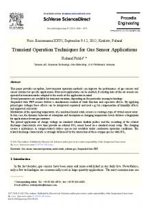
• Consensus Query: Given a fraction s ∈ (0, 1), find 0 all the values which are reported by more than sn 0 25 50 75 100 125 150 175 200 sensors. This can be thought of finding a value on which more than certain fraction of sensor agreed. Figure 4: A typical network routing tree for 40 nodes These values are called Frequent items. placed in a 200×200 area. We report all the unit-width buckets whose count are more than (s−ε)n. Since the count of leaf bucket has error in any q-digest and discard the query if it does not an error of at-most εn (Lemma 2), we will find all the satisfy the required precision. In experiments, for examvalues with frequency more than sn. There will be ple, we work with σ = 216 and m = 100, the theoretical a small number of false positives; some values with σ maximum error is 3 log ≈ 48%, but we get a confidence m count between (s − ε)n and sn may also be reported factor of ≈ 9% for the q-digest at the base station. This as frequent. leads to huge savings in terms of transmission cost. Notice that the actual error in query can still be much smaller than θ (in experiments the actual error in the median was 4.3 The Confidence Factor close to 2%). In Theorem 1 we proved that the worst case error for a qσ digest of size m is 3 log m . But this worst case occurs for a very pathological input set, which is unlikely in practice. 5 Experimental Evaluation Choosing the message size according to these estimates will lead to useless transmission of large messages, when We simulated our aggregation algorithm in C++. The sima smaller one could have ensured the same required error ulator takes the network topology (routing tree) and readbounds. So if the q-digest is computed by setting m to a ings of sensors as the input. The base station initiates qvalue for which it is expected to deliver the required error digest computation by sending a query to all its children, guarantees, we still need a way to certify that those guar- which forwards this query to their children, and so on. antees are met. For this, we provide a way to calculate the The leaf sensors send their value as q-digest to their parerror in each particular q-digest structure. We call this the ent. Each sensor then aggregates q-digests received from confidence factor. its children with its own reading, and then sends the agIf we define the weight of a path as the sum of the gregate to its parent. The quantile and range queries are counts of the nodes in the path, the weight of the path performed on the q-digest received at the base station. from root to any node is equal to the sum of its ancestors. The topology for the network was generated as follows. So the maximum error is present in the path of q-digest We assume that the sensors have a fixed radio range and with the maximum weight. We define the confidence fac- are placed in a square area randomly. If two sensors are tor θ as: θ = (maximum weight of any path from root to within range of each other, they are considered neighbors. leaf in Q) / n. This generates a network connectivity graph. The routing This ensures that the error in any quantile query is tree required for our simulation is simply a breadth first bounded by θ. Hence, now we can find out the maximum search tree over this graph with an arbitrary node chosen 9

We ran our aggregation algorithm for “random” and “correlated” sensor values. For the random case, each sensor value is taken to be a 16 bit random number. In a real network, the values at sensors are not random, but are correlated with their geographic location. To simulate such correlation we adapted geographic elevation data available from the United States Geological Survey (USGS) [21] which is shown in Fig 5. The sensors are assumed to be scattered over the terrain and the elevation of the terrain at the sensor location is assigned as the sensor value. The terrain size was scaled to fit in with our simulated terrain size and the elevation data was scaled to fit in 16 bits. All performance data we present is averaged over 5 different topologies.

Elevation

as the root or the base station. In Fig 4, we show a typical network routing tree. When we vary the number of sensors, we vary the size of the area over which they are distributed so as to keep the density of sensors constant. As an example, we used a 1000×1000 area for 1000 sensors with equal radio ranges. For 4000 sensors, the terrain dimensions were enlarged to 2000×2000 keeping radio range constant.

y x

Figure 5: Three dimensional elevation data for Death Valley which is used to model correlated data for our simulation. The bottom of the plot shows the contour lines for the terrain. Data Type Random Correlated Random Correlated

Msg Size (bytes) 160 160 400 400

θ 13% 24% 6.6% 7.3%

Actual Error 6.1% 5.0% 2.6% 1.9%

We compare the performance of our algorithm with a simple unaggregated data summarization scheme which we call list. In this scheme, the summary is a list of distinct sensor values and a count for each value. At each node, this list contains all the distinct sensor values that Table 1: Maximum possible error and actual error in meoccur in the subtree rooted at the node. In other words the dian query list structure is a histogram with bucket width 1. There is no information loss and we can answer quantile or histogram queries exactly. As the message progresses to- 5.2 Accuracy and Message Size wards the base station, more and more distinct values begin to occur and the size of the message grows. In an 8000 sensor network, we measured the accuracy of our algorithm in evaluating the median for different message sizes. The error in this experiment is defined as the ratio of rank error in the median estimated from q-digest and number of values (ε = (|r−n/2|) ). The results are 5.1 Range Queries and Histogram n shown in Fig 7. As expected, the graph shows that the erAs a first demonstration of our algorithm we build a his- ror declines very rapidly with growing message size and togram of the correlated input data using range queries with a message size of 160 bytes, we already are down to for 8000 nodes. We divided the data values into 32 equi- 5% error. There is no significant difference in error for width buckets and queried both q-digest and list sum- random or correlated data. We also calculated the confidence factors (θ) for memaries to find the number of values in each bucket. The dian calculation with varying message sizes. This data is resulting histogram is shown in Fig 6. On Fig 5 there are shown in Table 1. It is clear that the theoretically estitwo relatively flat areas which are clearly identifiable in mated accuracy is pessimistic compared to the actual acthe contour plot: the empty area near the bottom left hand curacy achieved. corner and the area near the center. Sensors on these areas will contribute a lot of values which are close to each Now we turn to a comparison of the message sizes reother. These features lead to two peaks (at 0 and 22K) in quired by q-digest and those required by list. From Fig 7 the histogram which are very well captured by our aggre- it is clear that a message size of 400 is sufficient to achieve gation scheme. accuracy of 2%. Compared to this, how much do we need 10

1200

25

exact q-digest

20 Percentage Error

Frequency

1000

correlated data random data

800 600 400

15 10 5

200 0

0 0

10K

20K 30K 40K 50K Sensar Data Value

60K

0

50

100

150 200 250 Message Size

300

350

400

Figure 6: Exact and approximate histogram of input data Figure 7: Measured percentage error in median vs messhown in Fig 5. The open boxes represent the exact his- sage size (in bytes) for an 8000 node network. togram while the solid thin bars represent the approximate histogram obtained from q-digest. near to the base station. Q-digest does a much better job at distributing load by requiring no node to transmit more to pay for exact answers? The comparison is shown in Fig than 400 bytes. 8 which shows maximum message size for q-digest and list for different numbers of sensors. Regardless of the correlation in data values or n (the number of sensors), to achieve 2% accuracy our maximum message size needs to be no bigger than 400. For random data, the size for list increases steadily with n. Since the sensor values for the random case can be any integer between 0 and 65535, the number of distinct sensor values is roughly proportional to the number of different sensors. For the correlated case, the number of distinct values in the input is only about 1500. So the maximum message size for list plateaus with increasing number of sensors. A more detailed view of the distribution of message sizes is shown in Fig 9. Given a message size m, we ask the question : what fraction of total nodes transmitted messages of size larger than m? This quantity is plotted in the vertical axis. We compare this distribution for list and q-digest (size 400 bytes) for random input values. For message sizes less than 400 bytes, the list and q-digest the distribution is identical. For q-digest there are no nodes which transmit message of size larger than 400 bytes. In comparison, about 5% (400 nodes) of nodes for the list scheme do transmit messages larger than this. 5% might look like a small number, but we immediately realize that these nodes actually bear an unusually heavy load. 1% of nodes transmit messages of size bigger than 3K and some nodes transmit messages of size up to 30K! These nodes represent nodes closer to the base station. In any routing tree most of the nodes are near the leaf levels and such nodes are very lightly loaded compared to nodes

5.3

Total Data Transmission

In Fig 10 we show the total amount of data transferred for q-digest and list. As expected, since the number of distinct values is less for correlated scenario, the amount of data transferred is lower for correlated data. For a network size of 1000, our scheme outperforms the list algorithm by a factor of 2, while for network size of 8000, this factor increases to about 4. This shows that our scheme is highly scalable, and has significant performance benefits in the case of larger networks.

5.4

Residual Power

Data transmission is very closely tied up with power consumption in sensor networks. There are two common metrics for measuring power consumption which we shall consider in turn.

11

• Total power consumption : This is the total power spent by all nodes in the network and is roughly proportional to total amount of data transmitted in the network (Fig 10). In reality, power consumption increases super-linearly with total data transmitted. This is because with increasing number of data packets, there is more contention for the wireless medium and a lot of power can be spent in packet collisions. • Lifetime : A more appropriate power consumption metric is the lifetime of the network. This is the time

30K

list-correlated list-random q-digest size-400

25K

1

list : random q-digest : random

20K 15K

Fraction of Nodes

Maximum Size of Message

35K

10K 5K 0 1000

2000

3000 4000 5000 6000 Number of Sensors

7000

8000

0.1

0.01

0.001

0.0001 Figure 8: Maximum message sizes for different numbers 1 10 100 1000 10000 100000 of sensors for naive unaggregated algorithm and our agMessage Size gregation algorithm. We fixed message size at 400 bytes which gives about a 2% error (see Fig 7). Figure 9: Cumulative Distribution of number of nodes as a function of message size. On the horizontal axis we have at which network partition occurs because of nodes message size m, while on the vertical axis we have numrunning out of power. A slightly different definition ber of nodes which transmitted messages of size larger of lifetime can be taken as the time required for the than m. Total number of nodes is 8000.

first node to run out of power. For a network which is geared towards data aggregation, the nodes near the base station shoulder the bulk of data transmission and hence runs out of power fastest. Thus in general, lifetime is a more useful indicator of the usable life of the network than total power consumption.

P =

100K

Total Data Transmitted

With q-digest, even nodes close to the base station transmit very small amounts of data and the transmission burden is distributed much more equitably. So we can expect the usable life time of the network to be vastly extended with our data aggregation scheme compared to the list scheme. We experimentally demonstrate this by considering the residual power of sensor nodes after a query. Let us assume that all nodes in the network start with the same amount of battery power. After a query has been processed, different nodes will have different amounts of power left depending on how much data each node transmitted. This power left is known as residual power. Residual power is a measure of the load distribution in the network. We simulated the effect of a single query on an 8000 node network where all nodes started out with equal power of 40000 units. We assumed that for every byte transmitted, one unit of power is depleted. The results are shown in Fig 11. On the horizontal axis we plot residual power fraction P which is defined as

80K

q-digest-random q-digest-corr list-random list-corr

60K 40K 20K 0 1000

2000

3000 4000 5000 6000 Number of Sensors

7000

8000

Figure 10: Total data transmitted plotted as a function of total number of sensors for both random and correlated input. The message size for the aggregated scheme was set at 160 bytes.

Residual Power Initial Power 12

1

q-digest list 1

q-digest list

Fraction of Nodes

0.1

0.1 0.01

0.01 0.988

0.001

0.99

0.992 0.994 0.996 0.998

1

0.0001 0

0.1

0.2

0.3

0.4

0.5

0.6

0.7

0.8

0.9

1

Residual Power Fraction

Figure 11: Cumulative distribution of nodes with residual power fraction. The inset shows a magnified view of the right hand edge of the graph. The total number of nodes is 8000, q-digest message size is 400. On the vertical axis we plot the number of nodes which have residual power fraction less than P . From Fig 11 we see that list does a very bad job of distributing load. More than one node (0.02% of 8000) have residual power fraction less than 1/2, i.e. one query drained half the battery power available for these nodes! At this consumption rate, after two queries using list, there will be at least one exhausted node. On the other hand q-digest performs well. The maximum message size for q-digest was set to 400; hence no node spent any more than 400 units of power. Thus all nodes had residual power fraction better than 99%. In the worst case, q-digest will be able to perform 100 queries before any node runs out of power.

query setting, such a digest will become outdated as sensor values change. It is possible to build a new q-digest by sending in a new query; but a more efficient way would be to send small updates such that the old q-digest can be refreshed with new information. In the current work, we have not taken into account the effect of lost messages. The effect of lost messages can be mitigated to some extent in a continuous query setting where the digest is continuously updated. In that case the parent can cache the q-digests received from its children and if a q-digest from a child is lost, it can replace that q-digest by the older one. As presented in this paper, q-digest provides information about the distribution of data values, but not information concerning where those values occurred. Since qdigest is easily extensible to multidimensional data, we are currently working on a multi-dimensional q-digest where spatial information will be preserved and hence the user would be able to query not only about data values, but the spatial locations of those values as well. We envision that as querying architectures for sensor network become more and more sophisticated, the use of efficient approximate algorithms will become very common.

References

6 Discussion and Future Work We have presented q-digest : a distributed data summarization technique for approximate queries using limited memory. It accurately preserves information about high frequency values while compressing information about low frequency ones. As such, it is a good approximation scheme when there are wide variations in frequencies of different values. Our experimental results indicate that orders of magnitude savings in bandwidth and power can be realized by q-digest compared to naive schemes for both random and correlated data. We note that q-digest is easily extensible to multidimensional data. For example to handle two dimensional data, we need to extend the binary tree representation of q-digest to a quad tree. We have shown how a q-digest can be computed in a distributed fashion once a query is made. In a continuous 13

[1] N. Bruno, S. Chaudhuri, and L. Gravano. STHoles: A Multidimensional Workload Aware Histogram. In Proc. of the 20th ACM SIGMOD Intl. Conf. on Management of Data (SIGMOD), 2001. [2] M. C. Burl, B. C. Sisk, T. P. Vaid, and N. S. Lewis. Classification Performance of Carbon BlackPolymer Composite Vapor Detector Arrays As a Function of Array Size and Detector and Composition, Sensors and Actuators, B, vol. 87 , pp 130-149, 2002 [3] L. Chen, D.W. McBranch, H.-L. Wang, R. Helgeson, F. Wudl, and D. G. Whitten. Highly sensitive biological and chemical sensors based on reversible fluorescence quenching in a conjugated polymer, Proc. National. Acad. of Science. vol. 96, pp 1228712292, 1999 [4] J. Considine, F. Li, G. Kollios and J. Byers. Approximate Aggregation Techniques for Sensor Databases, In Proc. of the 20th Intl. Conf. on Data Engineering (ICDE), 2004 [5] Crossbow http://www.xbow.com

Corporation,

[6] D. Estrin, R. Govindan, J. Heidemann and S. Kumar. [17] S. Madden, S. Szewczyk, M.J. Franklin and D. Next Century Challenges: Scalable Coordination in Culler. Supporting Aggregate Queries Over Ad-Hoc Sensor Networks, In Proc of the Fifth Intl. Conf. on Sensor Networks, Workshop on Mobile Computing Mobile Computing and Networks (MobiCom), 1999 and Systems Application, 2002 [7] The Firebug Project, [18] G. Manku and R. Motwani. Approximate frequency counts over data streams. In Proc. 28th Conf. on Very http://firebug.sourceforge.net Large Data Bases (VLDB), 2002 [8] J. M. Greenwald, and S. Khanna. Space-efficient [19] G. Piatetsky-Shapiro and C. Connell. Accurate EstiOnline Computation of Quantile Summaries. In mation of the Number of Tuples Satisfying a CondiProc. the 20th ACM SIGMOD Intl. Conf. on Mantion, In Proc. of ACM SIGMOD Intl. Conf. on Management of Data (SIGMOD), 2001 agement of Data (SIGMOD), 1984. [9] J. M. Greenwald, and S. Khanna. Power-Conserving [20] B. Przydatek, D. Song, and A. Perrig. Secure InforComputation of Order-Statistics over Sensor Netmation Aggregation in Sensor Networks, In Proc. of works. . In Proc. of 23rd ACM Symposium on Printhe First ACM Conf. on Embedded Networked Sysciples of Database Systems (PODS), 2004 tems (SenSys), 2003 [10] Habitat Monitoring on Great Duck Island, [21] The United States Geological Survey EROS Data http://www.greatduckisland.net/ Center, http://edc.usgs.gov/geodata/ [11] W. Heinzelman, Anantha Chandrakasan, and H. [22] Y. Yao and J. Gehrke, Query processing for Sensor Networks, In Proc. of the First Conf. on Innovative Balakrishnan. Energy-efficient Communication ProData Systems Research(CIDR), 2003 tocols for Wireless Microsensor Networks, In Proc. Hawaaian Int’l Conf. on Systems Science, January [23] Y. Yao and J. Gehrke, The Cougar Approach to In2000. Network Query Processing, ACM SIGMOD Record, vol. 31, pp 9, 2002 [12] J.M. Hellerstein, W. Hong, S. Madden , and K. Stanek. Beyond Average : Toward Sophisticated [24] J. Zhao, R. Govindan and D. Estrin. Computing AgSensing with Queries, In Information Processing gregates for Monitoring Wireless Sensor Networks, in Sensor Networks, eds. F. Zhao and L. Guibas, The First IEEE Intl. Workshop on Sensor Network Springer 2003. Protocols and Applications (SNPA), 2003 [13] J. Hill, R. Szewczyk, A. Woo, S. Hollar, and D. C. K. Pister. System Architecture Directions for Networked Sensors, In Proc. of Intl. Conf. on Architectural Support for Programming Languages and Operating Systems (ASPLOS), 2000 [14] C. Intanagonwiwat, R. Govindan and D. Estrin. Directed Diffusion: A Scalable and Robust Communication Paradigm for Sensor Networks, In Proc. of the Sixth Intl. Conf. on Mobile Computing and Networks (MobiCom), 2000 [15] James Reserve Microclimate and Video Remote Sensing, http://www.cens.ucla.edu [16] S. Madden, M.J. Franklin, J. Hellerstein and W. Hong. TAG: a Tiny AGgregation Service for AdHoc Sensor Networks, In Proc of 5th Annual Symposium on Operating Systems Design and Implementation (OSDI), 2002 14