Memory Neural Network For Kinematic Inversion Of

Proceedings of ICAR 2003 The 11th International Conference on Advanced Robotics Coimbra, Portugal, June 30 - July 3, 2003

Memory Neural Network For Kinematic Inversion Of Constrained Redundant Robot Manipulators B. Daˆachi+ , T. Madani+ , A. Ramdane-cherif∗ and A. Benallegue+ ∗ PRiSM, Universit´e de Versailles St.-Quentin 45, Avenue des Etats-Unis 78035 Versailles + Laboratoire de Robotique de Versailles 10, avenue de l’Europe 78140 V´elizy, France {[email protected], [email protected]} Abstract In this paper, we present an application of the cognitive approach to solve the problems related to the position controller using the inverse geometrical model. In order to control a robot manipulator to accomplish a task, trajectory planning is required in advance or in real time. The desired trajectory is usually described in Cartesian coordinates and needs to be converted to joint space for the purpose of analyzing and controlling the system behavior. In this paper, we use the memory neural network MNN to solve the optimization problem concerning the inverse of the direct geometrical model of the redundant manipulator subject to some constraints. Our approach offers substantially better accuracy, avoids the computation of the inverse or pseudoinverse Jacobian matrix and do not produce problems such as singularity, redundancy, and considerably increased computational complexity, etc.

1

Introduction

In recent years, artificial neural networks have received a great deal of attention for their ability to perform nonlinear mappings. In trajectory control of robotic devices, neural networks provide a fast method of autonomously learning the relation between a set of output states and a set of input states [1][2][3][4]. Since a neural network can only generalize within the range of information which has been presented to it, it will give an approximated solution near singularity points and therefore solve the singularity problem which has long been the major difficulty in implementing Resolved Motion Rate Control. Another problem that arise when studying the kinematic aspects of a robot manipulator is the so-called inverse geomtrical problem. In order to control a robot manipulator, using the position controller, to accomplish a task, trajectory planning is required in

1855

advance or in real time. The desired trajectory is usually described in Cartesian coordinates and needs to be converted to joint space for the purpose of analyzing and controlling the system behavior. The inverse gemetrical model can generally be approached by a numerical solution. The geometric method [5][6] derives a closed-form solution from the direct kinematic equation. For manipulators that do not have a closed-form solution like kinematically redundant manipulators, standard numerical procedures [7][6] solve the nonlinear differential equation at a discrete set of points. Moreover, for redundant arms, one solution has to be chosen from an infinite number of inverse kinematic solutions obtained for a given workspace position. This leads to an increased numerical complexity. The organization of this paper is as follows. In section 2, we recall the kinematic formulation of robot manipulator necessary to the inverse geometrical model of redundant robot subject to some constraints. Section 3 presents the topology of the neural network architecture MNN (memory neural network) and the learning method. Simulation results of a three DOF (degrees of freedom) robot arm are given in section 4. Finally some conclusions are drawn in section 5.

2

Kinematic formulation of the position based controller

In this section, we consider the kinematics of a redundant manipulator which has more degrees of freedom (DOF) than the dimension of the task space. Let q be a n × 1 vector of joint angles and x a m × 1 vector which represents the corresponding position of the end-effector in Cartesian coordinates (n > m). Then x and q are related by the forward kinematic transformation f (.) which is a well-known nonlinear function. Given (xd ) a trajectory of end-effector position in Cartesian space, the inverse problem is to compute

corresponding joint trajectories: position qd . Classical approaches consist in computing the solution by introducing the pseudoinverse matrix J + so that: ½

q = τ q˙ + q0 q˙ = J + x˙ + (I − J + J)v



 x1 F (q) = X(q) =  x2  x3   l1 c1 + l2 c12 + l3 c123 + · · · + ln c123···n =  l1 s1 + l2 s12 + l3 s123 + · · · + ln s123···n  g(q) (7)

(1)

For the purpose of the principle of our proposed method, we introduce an extended position vector as:

X = F (q) =

·

x 0

¸

=

·

f (q) g(q)

¸

x1 and x2 are the Cartesian coordinates in the plan (m = 2) and z is a vector of dimension (n − 2) and sij = sin(qi + qj ), cij = cos(qi + qj ). In general case:

(2)

where f(q) is the forward kinematic model and is g(q) the constraint vector added in the redundant case. These constraints can be represented by the general form proposed in Ballieul [9]

g(q) =

µ·

¸ ¶T ∂φ(q) =0 [N] ∂q

F (q) = X(q) = (x(q), z(q)) = (x1 (q), x2 (q), x3 (q), · · · , xm (q) , z1 (q), z2 (q), · · · zn−m (q))

(3)

φ(q) is a scalar kinematic objective function to be minimized and N is the (n − m) null space vector of J which corresponds to the self motion of a redundant arm: ˜ with N ˜= N = det(Ja )N

·

Ja−1 Jb −In−m

¸

(4)

Ja is a m−square matrix made of the m first columns of J and Jb a n× (n − m) matrix of the remaining columns: J = [Ja Jb ] and the (n − m) null space vector N of the J is obtained using (4), where the link lengths are l1 , l2 , · · · , ln . As the criterion φ(q) is convex with regard to q, we can conclude that the condition of optimality (3) is necessary and sufficient [9]. For our simulation, we choose the following objective function

(8)

The optimization problem consists to find the joint position vector q for a given Cartesian position vector (x, z). Generally z may be set to zero in order to find the optimal configuration that places the end-effector at the desired position x and minimizes the objective function φ(q). The robot arm must move in operational space thanks to commands that operate on the joint variables. Generally, the task that the manipulator must achieve is specified in operational space, space where it is easier to represent the movement of the robot. The passage from one space to another is thus very important and requires the direct and inverse models of the robot. These models are often very difficult to obtain because they are non-linear and time consuming. If we obtain the direct models relatively easily, the inverse models do not have, a priori, analytical expression. To find the inverse model is even more difficult if the robot is redundant (figure 1). q

F(q)

X

X(x,z)

?

q

n

φ(q) =

1X αi li (qi − q0i )2 2 i=1

(5) Figure 1: The extended direct and inverse model of a redundant manipulator.

This objective function aims to minimize joint displacement between two successive points. According to (4) and (5), the constraint equation becomes   w1 l1 (q1 − q01 )  w2 l2 (q2 − q02 )    (6) g(q) = N T  =0 ..   . wn ln (qn − q0n )

3

The extended forward kinematic equation for n DOF planar manipulator (m = 2 ⇒ redundancy equals to n − 2) is

1856

The neural network topology and the learning method

An efficient method to design Feedback Recurrent Network has been proposed in [10]. Here, we present a new neural method using Memory Neural Network. Neural networks have limitations in identifying complex plants. Indeed, they consist in neurons layers interconnected by weights, i.e., in static maps. The

usual way to build dynamic maps is to feedback outputs and delay inputs as much as necessary so that the input layer is made of the inputs and the outputs at different time instants. This Time Delay TDNN (figure 2) is intrinsically static and the learning phase is complicated by the feedback loops possibly raising stability problems.

model is resented in Fig.4. It consists of n inputs in the layer (E), c neurons in the hidden layer (H) and n neurons in the output layer (S). The E vector correspond to the Cartesian coordinates X = F (q) and the S vector correspond to the joint angle components (q). To each neuron of the hidden layer and of the output layer is connected, by a time delay, to a special neuron named memory neuron as is showed in Fig.3. Thus we obtain a new architecture of MNN Fig.4 (For simplicity, we do not represent the complete structure of the neuron as represented in Fig.3).

x0d(k) x0(k) x0(k-dt)

3.1

δ(k)

x0(k-2dt) δ(k-dt) δ(k-2dt)

Figure 2: Dynamic TDNN structure In Sastry [11] first introduced the concept of MNN (figure 3). To each neuron of a TDNN is added special neurons named memory neurons, witch are connected to their neurons by a time delay so that they are able to retain information. Sastry has proved MNN’s efficiency in automatic control especially for the identification of non linear dynamical systems. However, he kept the external feedback loop and therefore kept the same drawbacks.

Generalized MNN equations

Our learning database is composed by 2 vectors : inputs u, outputs y. W c , W mc , W bc are weights vectors for connections (neurons to neurons, memory cells to neurons, memory cell to itself) between layer c and layer c + 1, W 0 is chosen null to avoid direct relation between input and output. Bc is bias vector associated to neurons of the layer c (c 6= 0 : input layer). Ac is activation vector of layer c neurons, V c is non linear output function, Ac is output vector of neurons, and V mc is output vector of memory cells. N BCC is number of hidden layers (in our example N BCC = 1), NBC(c) is number of layer c neurons and N is value of the last layer (N = N BCC + 1).

Outputs S The output layer

Wc

H

The hidden layer

Wi

α

The input layer

Inputs

E

Figure 3: Sastry MNN Structure. Compared to TDNN, new MNN have many advantages: the absence of feedback loop allows the learning phase to be processed with a parallel structure (with the plant) witch is much simpler and avoids stability problems, and moreover, MNN is intrinsically dynamic. Each memory cell is a first order discrete time function and the hidden layer is a parallel structure of these dynamical functions. We have generalized MNN structures to understand their influence to learn and identify very complex non linear system. The architecture of MNN used to learn the inverse geometrical

1857

Figure 4: The NN architecture Equations for input layer: Vi0 = ui (k) V m0 (k) = M 0 V m0 (k − 1) + (I − M 0 )V 0 (k − 1) with M 0 = diagonal matrix(W b0 ) Equations for all hidden layer c from 1 to N BCC: V c (k) = f c (Ac (k)) Ac (k) = W m(c−1) V m(c−1) (k) + W (c−1) V (c−1) (k) + B c f is a sigmoid function. W and W m are vectors,

so: V c (k) = f c

(

S5

NBC(c−1) ³

X

m(c−1)r

Wj

m(c−1)

(k)Vj

=

(c−1)

Wj V

mc

c

(k) = M V

mc

c

(c−1)

(k)Vj c

(k)) + B c

c

(k − 1) + (I − M )V (k − 1)

´

)

M = Diagonal matrix (W bc )

Equation for the output layer N and the output s VsN (k) = AN s (k) m(N−1)T m(N−1) N−1T N−1 = Ws V (k) + Ws V +BsN

Js

=

Thus

L(X, ψ, W ) = PNBC(N) P 1

(

P

T

c c c + c=2 k ψk (V (k) − f S1 +S2 + S3 + S4 + S5 NBC(N)

S1

X

=

∂L ∂V c (k)

(c−1)

m(N−1)

− M N−1 ψk+1

=0

T

mc = ψkmc − M c ψk+1 − W mc Fkc+1 ψkc+1

= 0 For the layer 0 (particular case because W0 is null): ∂L ∂V c (k)

T

mc = ψkc − (I − M c )ψk+1 − W c Fkc+1 ψkc+1

= 0 ∂L ∂V m0 (k)

)

T

m0 = −W m0 Fk1 ψk1 + ψkm0 − M 0 ψk+1

= 0

)+B

(k)

T

mc = ψkc − (I − M c )ψk+1 − W c Fkc+1 ψkc+1

= 0 ∂L ∂V mc (k)

Recurrent equations for double back-propagation: These following formulas are placed in order of the spatial back-propagation (index c) from top to bottom and in order of the temporal back-propagation form right to left (index k). For the layer N-1:

j=1

(k)Vj

Partial derivatives For the layer N − 1:(particular case because no nonlinear function) PNBC(N) ∂L ((ys (k) − ysd (k))WsN−1 s=1 ∂V N−1 (k) =

For all hidden layer c with c from 1 to N − 2:

m(c−1)T m(c−1) (k)yj (k) j

(c−1)T

)

m(N−1)

(W

+Wj

(k) − M 1 V m1 (k − 1)

−(I − M 1 )V 1 (k − 1)

+ψk

(N−1)T N−1 y (k) k (((W s s=1 2NBC(N) m(N−1)T m(N−1) N d 2 +Ws y (k) + Bs ) − ys (k)) )

PN−1

m1

m(N−1)

NBC(N) X 1 Js N BC(N ) s=1 1X (ys (k) − ysd (k))2 2 k

=

(V

+ψkN−1 − (I − M N−1 )ψk+1 =0 PNBC(N) m(N−1) ∂L d = ((y (k) − y (k))W ) s s s s=1 ∂V m(N−1) (k)

Double Back-propagation Equations Equations of Lagrange Criterion: J

T

ψkm1

k

(k)+

j=1

T

X

c

NBC(N)

S2

=

X

T

ψkmc

(V

m(N−1)

mc

k

c

c

(k) − M V

mc

ψk

(k − 1)

s=1

−(I − M )V (k − 1) S3

=

X

T

S4

=

(

X k

(N−1)

NBC(0) T

(Wjm0 (k)Vjm0 (k) + B 1

ψk

)

ψkm1

(V

s=1

m1

((ys (K) − ysd (K))Wsm(N−1) ) m(N−1)

= (I − M N−1 )ψk+1 NBC(N)

−

j=1

T

X

= −

∀k

(at the last time K)

k

−f 1

m(N−1)

NBC(N) m(N−1)

ψK

ψk1 (V 1 (k) X

((ys (k) − ysd (k))Wsm(N−1) )

+M N−1 ψk+1

)

c

X

=

s=1

∀k

(k) − M 1 V m1 (k − 1)

X

((ys (k) − ysd (k))Ws(N−1) )

NBC(N)

(N−1) ψK

)

−(I − M 1 )V 1 (k − 1)

= −

X s=1

((ys (K) − ysd (K))Ws(N−1)

(at the last time K)

1858

d) Selected a new value of η from [ηmin ηmax ]and return to (a).

For the layer c from 1 to N − 2: ψkmc ψkc

T

mc = M c ψk+1 + W mc Fkc+1 ψkc+1

The equation (9) insure that η is not too large and equation (10) insure that η is not too small (ξ1 ∈]0 1[ and ξ2 ∈]ξ1 1[).

T

mc = (I − M c )ψk+1 + W c Fkc+1 ψkc+1

For the layer 0: T

ψkm0

m0 = M 0 ψk+1 + W m0 Fk ψk1 at the time k

4

T

m0 ψK

1 = W m0 FK ψK at the last time

Partial derivatives for the computation of gradient: At the optimum: ∇J ∂J ∂W ∂J ∂W 0 ∂L ∂WsN−1 ∂L ∂Wimc ∂L m(N−1) ∂Ws

∂L ∂W bc

∂L ∂B c ∂L and ∂BsN

= ∇L ⇒ © ª ∂L = ∀W ∈ W c , W mc , W bc , B c ∂W X ∂L = 0, =− Fk Vic (k)ψkc+1 c ∂Wi k

(with c from 1 to N − 2) X = (ys (k) − ysd (k))V N−1 (k) k

= −

X

Fk Vimc (k)ψkc+1

k

(with c from 0 to N − 2) X = (ys (k) − ysd (k))V m(N−1) (k) k

=

X ∂L =− (V mc (k − 1) c ∂M k

−V c (k − 1))ψkmc with c from 0 to N − 1 X = − Fk ψkc with c from 1 to N − 1

Simulation

For our simulation, we consider a three degrees of freedom planar robotic arm with links l1 = 2m., l2 = 1m. and l3 = 0.5m. The network is made up of one hidden layer, three input-layer neurons for the Cartesian coordinates (x1 , x2 , z), 15 neurons in the hidden layer, three neurons in the output-layer for the joint positions (q1 , q2 , q3 ). This neural network is trained on a set of Cartesian coordinates (x1 , x2 , z) which span the first quadrant of the manipulator’s workspace (1000 points). Substituting (x1 , x2 , z) in our algorithm [12], we obtain the output set of examples (q1 , q2 , q3 ). The initial weights are chosen randomly within the range -1 to +1. We have adopted the Sum Squared Error criterion (SSE) function of the iteration number to evaluate the training performance. We see that the MNN leads to a fast minimization of the criterion function. To verify generalization properties of the new architecture, the weight matrix obtained at the end of the learning phase is used. The test set is chosen out of the range of the learning set interval (500 pts). Tab.1 gives the test performance. By compared the SSE and the sum squared error (SSET) of the test we prove the good learning of the inverse geometrical model. Training set 1000 pts

k

X = (ys (k) − ysd (k)) k

The weights and the biases of the neural network are adjusted according to: Wk+1 = Wk + ηWk and Bk+1 = Bk + ∆Bk . The η is adjusted using the previous Goldstein rule. The one dimensional optimization with respect to the learning rate parameter is : ”Goldstein rule”: This rule can written as: ¯ ¯ putting ηmin = 0 and ηmax = 10 ¯ ˙ = ∇E t (W )P a) ¯¯ computing g(0) ¯ chosing initial value of η ¯ ¯ computing g(η) = E(W + ηP ) ¯ ˙ then go to (c) (9) b) ¯¯ if g(η) < g(0) + ξ1 ηg(0) ¯ else putting ηmax = η and go to (d) ¯ ¯ computing g(η) ˙ = g(0) and g(0) + ξ2 η g(0) ˙ ¯ ˙ End (10) c) ¯¯ if g(η) ≥ g(0) + ξ2 ηg(0) ¯ else ηmin = η

1859

SSE Test set 0.05 npt = 500 pts Test performance

SSET 0.08

Now, we use this neural network in the position control scheme as static maps to follow the straightline trajectory (x2 = −x1 + 2) while minimizing the performance criterion (q) defined in Eq.5. The results obtained for the tracking errors and criterion evolution are shown respectively Fig.5a and Fig.5b. The simulation gives a smooth joint trajectory which minimizes the objective function and follows the desired Cartesian trajectory. The tracking errors and the criterion evolution are little large at the beginning but very small for the whole trajectory. In order to illuminate the good behavior of this neural network controller compared to the analytical inverse Jacobian based controller (Resolved Motion Rate Control: RMRC) where Kv is the diagonal matrix of joint velocity loop gains and the command torque t can be calculated as: ˙ τ = Kv (J −1 Kp (Xd − X) − q)

(11)

0.03 0.02

0.15

ex1 0.1

0.01 0

0.95

z= NT(∂φ(q)/∂q)

0.05

x2

-0.01 -0.02

ex2

B

0.9

B 0.9

0.8 A

0.85

x2 0.8

0

0.6

-0.03

-0.05 0

10 20 30 40 50 60

a

-0.1

0

0.75

0.5

-0.05

A

0.4 0.7 0.75 0.8 0.85 0.9

10 20 30 40 50 60

b

(a)

Figure 5: (a) The Cartesian trajectory tracking error, (b) The criterion evolution

0.7

x1

0.8

0.95

x1 (b)

Figure 6: Figure-6- Results: (a) using the classical controller, (b) using the neural controller

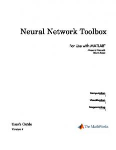
If Xd (t) lies inside the work envelope and does not go through singularities, then a joint space trajectory q˙d (t) can be obtained by q˙ = J −1 x˙ and the control torque is given by Eq.11. The singularities associated with the Jacobian matrix are often too complicated to be determined analytically. In order to provide an innovative solution to this singularity problem, we propose to use the previous Neural network in the position control scheme. For this purpose, the robot endeffector is commanded to follow various straight-line trajectories ( this robot has l1 = 2m, l2 = 0.5m, l3 = 0.5m). 1. The X1 (t) trajectory starts from point A at the neighborhood of a singularity (q2 = π ⇔ x1 = 0.71m, x2 = 0.71m). Fig.6a shows the robot end-effector motion using RMRC controller (dotted line). We see that this kind of controller leaves the manipulator uncontrolled since oscillations occur. Fig.6b shows the robot attempting to follow the same trajectory utilizing the neural network controller. This controller allows the whole trajectory to be achieved with small deviations at the beginning, near the singular point. 2. The X2 (t) starts from point C inside the manipulator workspace and tends to the workspace singular point D(q2 = 0 ⇔ x1 = 2.12m, x2 = 2.12m). Fig.7a and Fig.7b give the end-effector trajectory (dotted line) respectively using the inverse Jacobian based controller and the neural controller. The desired trajectory is represented in dashed line. With the first controller, the robot end-effector has an unexpected behavior near the boundary singularity while with the neural controller, it approximately follows the

1860

desired path. 2.1

2.14

D

2.12

D

2.12 2.1 2.08

x2

x2

2.06 2.04

2.04

2.02

2.02

2

2

C

1.98

2.05

2

(a)

x1

2.1

2.15

1.98

C 2

2.05

(b)

x1

2.1

2.15

Figure 7: Results: (a) using the classical controller (b), using the neural controller 3. The X3 (t) trajectory goes outside the manipulator workspace to the point E(x1 = 2.14m, x2 = 2.14m). The position response (Fig.8a) with the inverse Jacobian based controller shows very large deviations, the end-effector continuing its displacement anywhere in the workspace. With a neural controller (Fig.8b), the arm attempts to stay close to the desired trajectory. Hence, these results prove that the neural network controller compared to the classical RMRC scheme ensures a good trajectory tracking even near singularities. The performance of this controller only depends on the neural network accuracy to approximate the inverse extended geometrical function.

References 2.25

2.16

2.2

[1] A. Guez and Z.Ahmad. Accelerated convergence in the inverse kinematics via multiplayer feedforward networks. In IEEE International Conference on Neural Networks, pages 341-344, Washington, USA, June 1989.

E

2.14 2.12

E

2.15

x2

x22.1 2.08

2.1

2.06

[2] S. Kieffer, V. Morellas, and M. Donath. Neural network learning of the inverse kinematic relationships for a robot arm. In IEEE International Conference on Robotics and Automation, pages 2418—2425, Sacramento, California, USA, April 1991.

2.04 2.02

2

C

C

2

1.95 2

2.05

(a)

x1

2.1

2.15

2

2.05

(b)

x1

2.1

2.15

[3] A. Ramdane-Cherif, V. Perdereau, and M. Drouin. Acceleration of back-propagation for learning the forward and inverse kinematic equations. In ISNINC, The 2nd International Symposium on Neuroinformatics and Neurocomputers, Rostov-on-Don, Russia, September 1995.

Figure 8: Results: (a) using the classical controller (b) using the neural controller.

The neural network configuration is chosen using qualitative and quantitative assessment techniques. Our approach offers substantially better accuracy than classical methods and also better than other N N -based methods. In the literature we find only a few N N based methods applied to kinematics inversion problem. All these methods use generally the inverse Jacobean matrix to obtain the N N training set. Their accuracy at the vicinity of singularities is less performed. The number of neurons of the hidden layer is chosen using the analysis comparison technique for several trials which leads to find the number n as follows (I : number of inputs O : number of outputs): I 2 < n < 2O2 We have noticed that the fast minimization of the criterion function and the better accuracy of the MN N or N N depend mostly on the best selected training set.

5

Conclusion

In this paper, an artificial neural network is investigated for application to trajectory control problems in robotics. A MNN network is applied to learn the inverse geometrical model. Then is used in the position based controller for redundant robot subject to some constraints. Good results have been obtained: the tracking error is very small and the criterion is well minimized. This neural network can be used in other command structures and transformations. In this paper we showed that the cognitive approach through the neural network paradigm allows more to solve some complex problems which one cannot solve currently with conventional methods.

1861

[4] A. Ramdane-Cherif, V. Perdereau, and M. Drouin. Optimization schemes for learning the forward and inverse kinematic equations with neural network. In IEEE, International Conference on Neural Networks, Perth, Australia, Nov.Dec. 1995. [5] K. H. Hunt. Robot kinematics- a compact analytic inverse solution for velocities. ASME Journal of Mechanisms, Transmissions and Automation in Design, vol. 109, pp. 42-49, March 1987. [6] M. Kircanski and T. Petrovic, ’ Combined analytical-pseudoinverse inverse kinematic solution for simple redundant manipulators and singularity avoidance’, Int. Journal of Robotics Research, vol.12, no.1, pp.188-196, 1993. [7] R. Featherstone. Accurate trajectory transformations for redundant and non-redundant robots. IEEE International Conference on Robotics and Automation, pp.1867-1872, San Diego, USA, 1994. [8] Y. Bestaoui. An unconstrained optimization approach to the resolution of the inverse kinematic problem of redundant and non-redundant robot manipulators. Robotics and Autonomous Systems, 7, pp.37-45, 1991. [9] J. Baillieul. Kinematic programming alternatives for redundant manipulators. IEEE International Conference on Robotics and Automation, 1985, pp.722-728. [10] N. Chatry, V. Perdereau, M. Drouin, M. Milgram and J. C. Riat. A new design method for dynamical feedback networks. In proceedings of the In-

ternational symptium on soft computing for industry. ISSCI’96 (WAC’96), May 27-30, Montpellier, France, 1996. [11] P. S. Sastry, G. Santharam and K. P. Unnikrishnan. Memory neuron networks for identification and control of dynamical systems, IEEE, March 1994. [12] A. Ramdane-Cherif, V. Perdereau, and M. Drouin. Penalty approach for a constrained optimization to solve on-line the inverse kinematic problem of redundant manipulators. In IEEE International Conference on Robotics and Automation, Minneapolis, USA, April 1996.

1862