Meshless Computation of Water Hammer

Meshless Computation of Water Hammer

Arris S. TIJSSELING (corresponding author) Department of Mathematics and Computer Science Eindhoven University of Technology Den Dolech 2 P.O. Box 513, 5600 MB Eindhoven, The Netherlands Phone: +31 40 247 2755; Fax: +31 40 244 2489; Email: [email protected]

Anton BERGANT Litostroj E.I. d.o.o. Litostrojska 50 1000 Ljubljana, Slovenia Phone: +386 1 5824 284; Fax: +386 1 5824 174; Email: [email protected]

1

Abstract Water hammer concerns the generation, propagation, reflection and damping of pressure waves in liquidfilled pipe systems. The numerical simulation of water-hammer events is usually based on one-dimensional mathematical models. Two equations representing the conservation of mass and momentum govern the unsteady flow in the pipes. Boundary and/or intermediate conditions model the behaviour of hydraulic machinery and the additional complication of column separation. The method of characteristics is the preferred method of solution and the conventional approach is to define a fixed grid in the distance-time plane. On this grid, the unknown pressures and velocities (or heads and discharges) are numerically computed in a time-marching procedure that starts from a given initial condition. Rectangular or diamond grids are used that in general do not exactly match the given pipe lengths or the chosen time step. Therefore numerical interpolations and/or adjustments of wave speeds or pipe lengths are necessary, and these necessities introduce error. This paper presents a different way of water-hammer computation. The procedure is based on the method of characteristics, but a numerical grid is not required. Any point in the distance-time plane can be selected to compute the local solution without explicitly using stored previous solutions. The computation is based on back-tracking waves by means of a very simple recursion, so that the programming effort is small. Exact solutions are thus obtained for frictionless water-hammer. Approximate solutions are obtained when the distributed friction in individual pipes is concentrated at the pipe boundaries. The new algorithm is fully described and the new method is evaluated and compared with conventional water-hammer calculations. The following boundary conditions are tested: reservoir, instantaneous and gradual valve closure, and pipe junction. The algorithm is easy to implement and its exact solutions can be used to asses the numerical error in more conventional methods for the test cases of frictionless waterhammer and lumped friction.

Key words Unsteady pipe flow; Hydraulic transients; Pressure surges; Water hammer; Wave propagation; Wave reflection; Method of characteristics; Mesh-free method; Exact solution.

2

1.

Introduction

1.1.

Water-hammer equations

Classical water-hammer theory [1-7] adequately describes the low-frequency elastic vibration of liquid columns in fully-filled pipes. The pipes are straight, prismatic, thin-walled, linearly elastic and of circular cross-section. The two equations, governing velocity, V, and pressure, P, are

∂V ∂t ∂V ∂z

+

+

1 ∂P

ρ ∂z 1 ∂P K

*

∂t

= − f

VV

,

(1)

4R

=0 ,

(2)

with

1 K

*

=

1

+

K

2R

.

(3)

Ee

Notation: E = Young modulus, e = wall thickness, f = Darcy-Weisbach friction factor, K = bulk modulus, K* = effective bulk modulus, R = inner pipe radius, t = time, z = distance along pipe, and ρ = mass density. The pressure wave speed is

c =

1.2.

K

*

ρ

.

(4)

Conventional methods of solution

The method of characteristics (MOC) is the preferred technique to solve the water-hammer equations [8-9], because the wave speed c is constant and, unlike finite-difference [10-11], finite-volume [12-13], finiteelement [14-15] and lattice-Boltzmann [16] methods, steep wave fronts can be properly dealt with. The distance-time (z-t) plane is covered with either a rectangular (collocated) or a diamond (staggered) computational grid in accordance with the Courant condition ∆ x = c ∆t . Horizontal-vertical [1-7] or diagonal [17] time-marching from a known initial condition gives approximate and exact solutions in systems

3

with and without friction, respectively. In multi-pipe systems the Courant condition cannot be satisfied in all pipes if a common time step ∆t is adopted, and wave-speed or pipe-length adjustments and/or interpolations have to be applied. These introduce numerical error. In single pipes, interpolations are necessary when numerical data is required in between grid points, for example at the exact location of measuring equipment. Wood et al. [18, 19] developed and commercialised an alternative MOC-based solution procedure. Closedform analytical solutions can be obtained for water hammer in a single pipe with lumped [20] or linearised [21] friction.

1.3.

New algorithm

The new approach presented in this paper has no adjustments (of wave speeds or pipe lengths), no numerical interpolations and no approximations (except for lumped friction). The method automatically tracks waves backward in time by means of a simple recursion. The exact solutions obtained for frictionless water-hammer in multi-pipe systems can be used: to check numerical results and schemes, to serve as reference solutions in benchmark problems, and to perform parameter variation studies without parameter changes generated by the numerical method itself (e.g. changed wave speeds or pipe lengths). The method is mesh-free in the sense that a conventional computational grid is not required. The theory is presented in general form so that it can be applied to analogous two-equations systems in, for example, open channel flow, structural vibration, and electronics. It can be extended to four-equation systems encountered in, for example, the theory of linear(ised) waves in two-phase flows, two-layer density currents, liquid-saturated porous media, and water hammer with fluid-structure interaction [22]. The method even works for higher-order systems like those developed for water hammer by Bürmann [23], noting that then the necessary eigenvalues and eigenvectors cannot be found in closed form.

2.

Theory

2.1.

General hyperbolic equations

4

The general linear equations

A

∂

φ( z ,t ) + B

∂t

∂ ∂z

φ( z ,t ) + C φ( z ,t ) = 0

(5)

describe wave propagation in one spatial dimension. The constant matrices A and B are invertible and A−1 B is diagonalizable. The constant matrix C, which may be non-invertible, causes frequency dispersion (if C ≠ O). The N dependent and coupled variables φi , constituting the state vector φ , are functions of the independent variables z (space: 0 ≤ z ≤ L) and t (time: t ≥ 0). Herein N = 2 and C = O.

2.2.

Method of characteristics (MOC)

The MOC introduces a new set of dependent variables through

η ( z , t ) = S −1 φ ( z , t )

or

φ( z ,t ) = S η( z , t ) ,

(6)

so that each ηi is a linear combination of the original variables φi . Substitution of (6) into (5), with C = O, gives

AS

∂ ∂t

η( z , t ) + B S

∂ ∂z

η( z ,t ) = 0 .

(7)

Multiplication by S−1A−1 yields

∂ ∂t

η( z ,t ) + Λ

∂ ∂z

η( z ,t ) = 0 ,

(8)

in which −1

−1

Λ =S A BS .

(9)

A set of decoupled equations is obtained when Λ is diagonal:

 λ1

0 

0

λ2 

Λ =

.

(10)

Substitution of (10) into (9) and solving for S reveals that a non-trivial solution exists only when the diagonal elements of Λ are eigenvalues satisfying the characteristic equation

det ( B − λ A ) = 0 ,

(11)

5

in which case S consists of the eigenvectors ξ i belonging to λ i :

S = ( ξ1 ξ 2 ) .

(12)

The decoupled equations (8),

∂ η i ( z ,t ) ∂t

+ λi

∂ ηi ( z ,t ) ∂z

=0 ,

i = 1, 2 ,

(13)

transform to

d ηi ( z , t )

=0 ,

i = 1, 2 ,

(14)

dt when they are considered along characteristic lines in the z-t plane defined by

dz dt

= λ i , i = 1, 2 .

(15)

The solution of the ordinary differential equations (14) and (15) is

η i ( z , t ) = η i ( z − λ i ∆t , t − ∆ t ) ,

i = 1, 2 ,

(16)

when a numerical time step ∆t is used, or, more general and with reference to Fig. 1,

η i ( P ) = η i ( Ai ) , i = 1 , 2 ,

 η ( A1 )  η ( P) =  1  . η 2 ( A 2 ) 

or

(17)

The value of the unknown variable ηi does not change along the line Ai P. The original unknowns in φ are obtained from η through (6). This gives 2

φ(P) =

∑ S R i S −1

φ ( Ai ) ,

(18)

i =1

where the i-th diagonal element of the matrix R i is 1 and all other elements are 0.

2.3.

Boundary conditions

At the boundaries at z = 0 and z = L, the relations (16) or (17) provide just one equation (see Fig. 2). To find the two unknowns ηi (P), i = 1, 2, at z = zb (zb = 0 or zb = L), one additional equation per boundary is required. These are given by the linear boundary conditions

d Tz (t ) φ( zb , t ) = qz (t ) b

b

or

d Tz (t ) S η( zb , t ) = qz (t ) , b

b

6

(19)

where d Tz is a row vector with 2 coefficients and the scalar qz is the (boundary) excitation. For b

b

convenience, the two row vectors d T0 and d TL are stacked in the 2 by 2 matrix D, and the vector q consists of the two scalars q1 = q0 and q2 = qL. Section 2.6 gives an example of matrix D.

Fig. 1 Interior point P and "feeding" characteristic lines in the distance-time plane.

Fig. 2 Boundary point P and "feeding" characteristic line in the distance-time plane.

7

2.4.

Junction conditions

At junctions at z = zj the unknowns ηi (P) may be discontinuous. The relations (16) or (17) provide two equations for ηi (P ± ) , i = 1, 2 (see Fig. 3). Two additional equations are required to find the unknowns at both sides of the junction, z = z j − and z = z j +. These are given by the linear junction conditions

J1(t ) φ ( z j− , t ) = J2(t ) φ ( z j+ , t ) + r (t )

or

J1(t ) S1 η1 ( z j , t ) = J2(t ) S2 η2 ( z j , t ) + r (t ) ,

where J1 and J2 are 2 by 2 coefficient matrices and the vector r is the (junction) excitation. Section 2.6 gives an example of J1 and J2. Thus the state vector φ can be discontinuous at z = z j . In general, the Riemann invariants η1 = S1 −1 φ and η2 = S2 −1 φ in the domains left and right of the junction are different. Only if J1(t ) S1 = J2(t ) S2 the junction will not cause wave reflection.

Fig. 3 Junction point P and "feeding" characteristic lines in the distance-time plane.

8

(20)

2.5.

Initial conditions

The initial condition at t = 0 can be the steady-state solution φ ( z ,0) = φ0 , where the constant state φ0 is consistent with the boundary and junction conditions, or it can be any non-equilibrium state φ ( z ,0) = φ0 ( z ) exciting the system (e.g. sudden release of pressure).

2.6.

Water-hammer two-equation model

In terms of the general equation (5), frictionless water-hammer [Eqs. (1-2) with f = 0] is represented by the state vector

V  φ=  P

(21)

and the matrices of coefficients

0  1 A =  * −1   , 0 K 

(22)

 0 ρ −1  B =   . 1 0 

(23)

The characteristic (dispersion) equation (11), corresponding to the matrices (22) and (23), yields

λ1,2 2 =

K*

ρ

= c2 ,

(24)

where λ1 is positive and λ2 is negative. The transformation matrix used [Eq. (12)] is S = ( TA )

–1

with T defined by

1 ( ρ c) −1   1 λ1  −1 T=  .  , so that S =  1 λ 2  1 −( ρ c) −1     

(25)

It is noted that transformation matrices are not unique. For example, S = ( TB )

–1

is an equally valid

transformation matrix. The boundary conditions are defined through coefficient matrix D and excitation vector q [see Eq. (19)]. For example, a reservoir at z = 0 and a valve at z = L, as in the test problems in Section 4, are represented by

9

d T0 = ( 0 1)

and

q 0 = Pres ,

(26)

d TL = (1 0 )

and

qL = 0 ,

(27)

where Pres is the reservoir pressure. Now Eqs. (26) and (27) are combined to give

0 1 D=  1 0

and

P  q =  res  .  0 

(28)

The junction conditions are defined through coefficient matrices J1 and J2, and excitation vector r [see Eq. (20)]. For example, continuity of flow rate and pressure at the junction of two pipes requires that

 A1 0  J1 =  ,  0 1

 A2 J2 =   0

0  1

and

0 r=  , 0

(29)

where A1 and A2 are the cross-sectional pipe areas left and right of the junction.

2.7.

Nonlinear non-instantaneous valve closure

In steady turbulent pipe flow the pressure loss, ∆ P0 , across a fully open valve is given by the orifice equation

∆ P0 = ξ0 12 ρ V0 V0 ,

(30)

where ξ 0 is an empirical loss coefficient [4, pp. 44-45]. The same relation is assumed to hold for a closing valve,

∆P = ξ

1 2

ρV V ,

(31)

where ξ depends on valve position and hence of time. Division of (31) by (30) and introduction of the dimensionless valve closure coefficient τ = ξ 0 / ξ gives the nonlinear boundary condition

P0 V V = τ 2 (t ) V0 V0 P ,

(32)

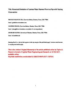
where the pressure downstream of the valve has been taken zero, so that ∆ P0 = P0 and ∆ P = P . The specific function τ (t ) used herein is  (1 − t / Tc ) 3.53 for 0 ≤ t ≤ 0.4 Tc  τ ( t ) =  0.394 (1 − t / Tc )1.70 for 0.4 Tc ≤ t ≤ Tc ,  0 for t ≥ T c 

(33)

10

in which Tc is the valve closure time and ξ 0 = 0.2 (see Fig. 4). This function, which is based on measured ball-valve discharge coefficients, was provided by Professor DC Wiggert (Michigan State University, USA) to Delft Hydraulics (The Netherlands) in 1987. More information on ball-valve discharge characteristics can be found in [24-25]. The quadratic equation (32) is solved simultaneously with one linear equation (one compatibility equation). This is done exactly in Appendix A. In using the quadratic formula for (32), care should be taken of possible cancellation [26]. The resistance of the valve in steady state leads to a small initial pressure, so that

 V0  φ0 =   ,  P0 

(34)

with P0 equal to Pres to ensure initial equilibrium.

tau (-)

1

0.5

0

0

0.01 0.02 time (s)

0.03

Fig. 4 Valve-closure function τ(t) for Tc = 0.03 s.

11

2.8.

Modelling of friction

Distributed friction (f > 0) is modelled by lumping it to one of the pipe ends, which is the common procedure in graphical [27] and wave-plan [18] methods. For example, the pressure loss at a reservoir-pipe entrance is then represented by the boundary condition [4, p. 103]

Pres − P = (1 + k + f

L ρV V ) 2R 2

,

(35)

where k is the (minor) entrance loss and L is the pipe length. The term 1+k is neglected herein.

2.9.

Modelling of column separation

Column separation [28] occurs when the absolute pressure drops to the vapour pressure Pv . This can be modelled at closed pipe ends by adopting the boundary condition P = Pv as long as the cavity volume ∀ is positive. The calculation of ∀ through

∀ (t ) =∀ (t − ∆t ) ± A V (t ) ∆t

(36)

can only be done by explicitly storing (and interpolating) previous cavity volumes.

3.

Algorithm

This section with its two appendices is the heart of the paper. It describes an algorithm for finding the exact value of the state vector φ in any point (z, t) in the distance-time plane. The algorithm is formulated in terms of the Riemann invariants ηi , i = 1, 2 , and it is based on a "coast-to-coast" approach, which is explained in words now. Figure 2 is essential. The vector η in point P on the left boundary at z = 0 at time t consists of the two components η 1 and η 2. The component η 2 is assumed to be known because, according to equation (17), it is equal to η 2 in the point A2, on the right boundary at z = L. The component η 1 follows from the boundary condition (19) and it depends on d T0 , S, q0 and η 2. Naturally, the same story holds for any point P on the right boundary. For the calculation of η in point P on the left boundary, one needs information from the "earlier"

12

point A2 on the right boundary; and for the calculation of η in the point A2 on the right boundary, one needs information from the "earlier" point A1 on the left boundary. This whole process can nicely be captured in a simple recursion that stops when characteristic lines intersect the t = 0 line, at which η has a given initial value. The recursion and the treatment of internal points (Fig. 1) are presented for a single pipe in Appendix B. The treatment of junctions (Fig. 3) and double pipes is similar and dealt with in Appendix C.

4.

Results

The new method is validated through the calculation of some basic results for frictionless water-hammer. The obtained exact solutions give details as fine as the chosen resolution in time or distance. Conventional MOC results obtained on very fine computational grids are given as a control.

P IP E

R E S E R V O IR

VALVE

Fig. 5 Single-pipe test problem.

4.1.

Single pipe

The single-pipe test problem [22] sketched in Fig. 5 is a water-filled reservoir-pipe-valve system defined by: L = 20 m, R = 398.5 mm, e = 8 mm, E = 210 GPa, K = 2.1 GPa, ρ = 1000 kg/m3, f = 0, and Q0 = 0.5 m3/s, so that the initial flow velocity V0 = 1.002 m/s and the wave speed c = λ1 = −λ2 = 1025.7 m/s [Eq. (24)]. A pressure transducer (PT) is assumed to be located at distance z = 11.15 m from the reservoir. Rapid closure of

13

the valve generates the Joukowsky pressure P = ρ cV0 = 1.028 MPa only if the closure time Tc is smaller than the wave reflection time 2L/c. This is the case for the pressure histories (taken relative to a constant static pressure high enough to prevent the occurrence of cavitation) portrayed in Fig. 6. The classical case of instantaneous valve closure is shown in Fig. 6a. Figure 6b, which is for non-instantaneous valve closure with Tc = 0.03 s, reveals that the pressure effectively starts to rise after time 0.7Tc . Figure 7 displays the corresponding pressure distribution along the pipe at time t = 0.24 seconds. The results in Figs. 6 and 7 were obtained with the new method and with the conventional MOC method utilising a very fine computational grid (924 reaches and a time step of 21 microseconds) and a marginally changed wave speed c = 1025.3 m/s. Both solutions are displayed in the Figs. 6 and 7, but the differences are hardly visible, thus confirming the validity of the new method. The new method calculated solutions in 240 points in time (1 millisecond step) to produce Fig. 6 and in 240 reaches to produce Fig. 7. These values were chosen to obtain high resolution, not high accuracy, because exact solutions are always obtained. It is noted that finding exact solutions for frictionless water-hammer in a single pipe is nothing special, except that the

pressure (Pa)

exact solutions are not necessarily in equidistantly spaced grid points.

1.5 .10

6

1 .10

6

5 .10

5

0 5 .10

5

1 .10

6

1.5 .10

6

0

0.05

0.1 0.15 time (s)

(6a)

14

0.2

pressure (Pa)

1.5 .10

6

1 .10

6

5 .10

5

0 5 .10

5

1 .10

6

1.5 .10

6

0

0.05

0.1 0.15 time (s)

0.2

(6b)

Fig. 6 Single-pipe test problem. Pressure history calculated at z = 11.15 m: (a) Tc = 0 s, (b) Tc = 0.03 s.

pressure (Pa)

Solid line: new method. Dotted line: conventional method.

1.5 .10

6

1 .10

6

5 .10

5

0

0

2

4

6

8 10 12 distance (m)

(7a)

15

14

16

18

20

pressure (Pa)

0 5 .10

5

1 .10

6

1.5 .10

6

0

2

4

6

8 10 12 distance (m)

14

16

18

20

(7b)

Fig. 7 Single-pipe test problem. Pressure distribution along the pipe calculated at t = 0.24 s: (a) Tc = 0 s, (b) Tc = 0.03 s. Solid line: new method. Dotted line: conventional method.

1 1 .1 5

3 .8 5

20 0 .8

0

zj

PT

L

Fig. 8 Double-pipe test problem. Distances in metres.

4.2.

Double pipe

In the double-pipe test problem sketched in Fig. 8, the first 3.85 m of the pipeline has a twice thicker wall (e1 = 16 mm, e2 = 8mm). The wave speed in the thick section is c1 = 1184.0 m/s, which is larger than c2 = 1025.7 m/s. The calculated pressure histories are shown in Fig. 9. The instantaneous valve closure in Fig. 9a clearly brings out all the reflections from the thicker pipe at the inlet. Joukowsky’s value is exceeded and a

16

beat is starting to develop. The mathematical challenge is to capture all the tiny peaks in the entire period of simulation. The new method is able to do so, because it is exact. The traditional water-hammer simulation can only achieve this by using again a very fine computational grid of 900 reaches with a time step of 21 microseconds, and marginally changed wave speeds c1 = 1184.3 m/s and c2 = 1025.5 m/s. The new method used a time step of 500 microseconds to produce Fig. 9 and 480 reaches to produce Fig. 10. Figure 9b is the more realistic case of gradual valve closure. All tiny peaks are smeared out now, but Joukowsky is still exceeded and a beat still develops. Figure 10 is the pressure distribution along the pipeline at time t = 0.24 seconds. Both new and conventional solutions are displayed in the Figs. 9 and 10, but the differences are hardly visible, thereby confirming again the validity of the new method. Finding exact solutions for frictionless

pressure (Pa)

water-hammer in a double pipe is − to the author’s knowledge − new.

1.5 .10

6

1 .10

6

5 .10

5

0 5 .10

5

1 .10

6

1.5 .10

6

0

0.05

0.1 0.15 time (s)

(9a)

17

0.2

pressure (Pa)

1.5 .10

6

1 .10

6

5 .10

5

0 5 .10

5

1 .10

6

1.5 .10

6

0

0.05

0.1 0.15 time (s)

0.2

(9b)

Fig. 9 Double-pipe test problem. Pressure history calculated at z = 11.15 m: (a) Tc = 0 s, (b) Tc = 0.03 s. Solid line: new method. Dotted line: conventional method.

18

pressure (Pa)

1 .10

6

8 .10

5

6 .10

5

4 .10

5

2 .10

5

0 2 .10

5

4 .10

5

6 .10

5

0

2

4

6

8 10 12 distance (m)

14

16

18

20

8 10 12 distance (m)

14

16

18

20

(10a)

pressure (Pa)

0 2 .10

5

4 .10

5

6 .10

5

8 .10

5

1 .10

6

1.2 .10

6

1.4 .10

6

0

2

4

6

(10b)

Fig. 10 Double-pipe test problem. Pressure distribution along the pipeline calculated at t = 0.24 s: (a) Tc = 0 s, (b) Tc = 0.03 s. Solid line: new method. Dotted line: conventional method.

19

5.

Conclusion

The equations for water hammer without friction have been solved exactly for time-dependent boundary and constant (steady state) initial conditions with a new method based on the MOC. The strength of the method is the simplicity of the algorithm (recursion) and the fast and accurate (exact) calculation of transient events. Its weakness is that the calculation time strongly increases for events of longer duration. The solutions are exact for the selected points of calculation in the distance-time plane, but they do not give information on what exists in between these points (no guaranteed constant values as in methods that track discontinuities). The efficiency of the algorithm can be much improved because many repeat calculations occur, but this will be at the expense of simplicity and clarity. The method is mesh-free and ideal for parallellisation and adaptivity. It is highly suitable to quickly calculate a limited number of exact transient pressure histories and distributions in simple frictionless pipe systems. The new method has been successfully validated against conventional water-hammer software in two simple test problems. In the second test problem, for the first time, an exact solution for frictionless waterhammer in a two-pipe system is presented.

20

Nomenclature

Scalars A

cross-sectional area, m2

c

pressure wave speed, m/s

det

determinant

E

Young modulus of pipe wall material, Pa

e

pipe wall thickness, m

f

Darcy-Weisbach friction factor

K

bulk modulus, Pa

K*

effective bulk modulus, Pa

k

minor (entrance) loss

L

pipe length, m

P

pressure, Pa

Q

flow rate, m3/s

qz

b

boundary excitation

R

inner radius of pipe, m

Tc

valve closure time, s

t

time, s

V

velocity, m/s

∀

cavity volume, m3

z

axial coordinate, m

∆

numerical step size; change in magnitude

λ

eigenvalue, wave speed, m/s

ξ

valve loss coefficient

ρ

mass density, kg/m3

τ

valve closure function - see Eq. (33)

21

Matrices and Vectors A

coefficients - see Eqs. (5) and (22)

B

coefficients - see Eqs. (5) and (23)

C

coefficients - see Eq. (5) and C = O herein

D

boundary condition coefficients - see Eqs. (19) and (28)

d Tz

row of matrix D

J1, J2

junction condition coefficients - see Eqs. (20) and (29)

O

zero matrix

q

boundary excitation vector - see Eqs. (19)

R

matrix - see Eq. (18)

r

junction excitation vector - see Eqs. (19)

S

transformation matrix - see Eqs. (12) and (25)

T

transformation matrix - see Eq. (25)

Λ

diagonal matrix of eigenvalues - see Eq. (10)

η

Riemann invariants - see Eq. (6)

ξ

eigenvector - see Eq. (12)

φ

dependent variables - see Eqs. (5) and (21)

b

Subscripts b

boundary

j

junction

L

boundary position z = L

res

reservoir

v

vapour

0

boundary position z = 0; initial state t = 0

Extensions 1

pipe 1

2

pipe 2

22

Appendix A

Solution of nonlinear equation (32)

The nonlinear boundary condition (32) is solved simultaneously with one linear equation for the two variables V and P. The system of equations can be written as

a1 V + a2 P = a3 ,

(37a)

b1 V 2 + b2 P = b3 ,

(37b)

where the coefficients ai and bi (i = 1, 2, 3) can be time dependent and a2 ≠ 0 and b1 ≠ 0 . Elimination of P gives

a2 b1 V 2 − a1 b2 V + a3 b2 − a2 b3 = 0 ,

(38)

so that 1

a b ± {a12 b22 − 4 a2 b1 (a3 b2 − a2 b3 )}2 V = 1 2 . 2 a2 b1

(39)

This formula is susceptible to numerical error, because of cancellation [26]. In the present paper the coefficients in (37) for the single pipe are 1 a1 = S −11 ,

1 a2 = S −12 ,

a3 = η1 (A1 ) ,

b1 = ± 1 ,

b2 = −τ 2 (t ) V 0 V 0 / P0 ,

b3 = 0 ,

and for the double pipe these are 1 a1 = S2 −11 ,

1 a2 = S2 −12 ,

a3 = η 21 ("A1 ") ,

b1 = ± 1 ,

b2 = −τ 2 (t ) V 20 V 2 0 / P 20 ,

b3 = 0 .

The matrices S and S2 are given by (25) and the function τ(t) by (33). According to relation (32), which describes positive flow (in z-direction) for positive pressure P, the following condition must hold:

b1 V ≥ 0 .

(40)

In the examples presented herein, b1 = + 1 and the + sign (+ root) in (39) gave valid solutions satisfying condition (40).

23

Appendix B

Recursion for a single pipe

Input

The coefficient matrices A, B, D(t), the excitation vector q(t), the initial condition φ0 ( z ) , the length L, and the positive wave speed λ1 = −λ2 describe the complete single-pipe system in general terms. It is stressed once again that C = O in Eq. (5), so that the algorithm does not apply to systems with distributed friction, viscous damping, etc.

Output

The output is the state vector φ = Sη as a function of distance and time.

Boundary points

See Figure 2. The subroutine BOUNDARY calculates η in the boundary points (finally) from constant initial values. The pseudo-code reads:

BOUNDARY (input: z, t ; output: η) if (t ≤ 0) then

η := η 0 else if (z = 0) then CALL BOUNDARY (L, t + L / λ2 ; η)

η2 := η 2

η 1 := α12(t) η2 + β11(t) q1(t) η 2 := η2

24

if (z = L) then CALL BOUNDARY (0, t – L / λ1 ; η)

η1 := η 1

η 1 := η1 η 2 := α21(t) η1 + β22(t) q2(t) if (z ≠ 0 AND z ≠ L) then "z is not at a boundary" end

Note that λ2 is a negative number herein. The coefficients α and β are given in Table 1. They define the unknowns η 1 and η 2 at the left and right boundaries, respectively, as the exact solution of the linear equation (19). For the case of nonlinear non-instantaneous valve closure, as described in Section 2.7, in subroutine BOUNDARY: q2 (t ) = V from Eq. (39), for z = L.

Interior points

See Figure 1. The subroutine INTERIOR calculates η in the interior points from the boundary values. The pseudo-code reads:

INTERIOR (input: z, t ; output: η) if (0 < z < L) then CALL BOUNDARY (0, t – z / λ1 ; η)

η1 := η 1 CALL BOUNDARY (L, t – (z−L) / λ2 ; η)

η2 := η 2

η 1 := η1 η 2 := η2

25

else "z is not an interior point" end

Implementation

The algorithms have been implemented in Mathcad 11 [29]; the interested reader may find the Mathcad worksheet in Appendix D.

z=0 α12( t ) :=

z=L

−DS ( t) 1 , 2

α21( t ) :=

DS ( t ) 1 , 1 β11( t) :=

1

DS ( t) 1 , 1

−DS ( t) 2 , 1

DS ( t ) 2 , 2 β22( t) :=

1

DS ( t) 2 , 2

Table 1 Definition of the coefficients α and β in subroutine BOUNDARY. DS(t) is the matrix product of D(t) and S.

26

Appendix C Recursion for a double pipe

Input

The coefficient matrices A1, B1, A2, B2, D(t), J1(t), J2(t), the excitation vectors q(t) and r(t), the initial conditions φ1 0 ( z ) and φ 2 0 ( z ) , the lengths z j and L, and the positive wave speeds λ11 = −λ12 and λ21 =

−λ22, describe the complete double-pipe system in general terms. The extensions 1 and 2 in the notation refer to the domains left and right of the junction at z = z j . See Figure 3.

Output

The output is the state vector φ = Sη as a function of distance and time, with φ = S1 η1 if 0 ≤ z ≤ z j− and φ = S2 η2 if z j+ ≤ z ≤ L .

Boundary and junction points

See Figure 3. The subroutine BOUNDARY calculates η1 and η2 in the boundary and junction points (finally) from constant initial values. The pseudo-code reads:

BOUNDARY (input: z, t ; output: η1, η2) if (t ≤ 0) then

η 1 := η1 0 η 2 := η2 0 else if (z = 0) then CALL BOUNDARY (z j, t + z j / λ12 ; η1, η2)

η2 := η1 2

27

η11 := α12(t) η2 + β11(t) q1(t) η1 2 := η2 if (z = L) then CALL BOUNDARY (z j, t – (L–z j) / λ21 ; η1, η2)

η1 := η 2 1

η 2 1 := η1 η 2 2 := α21(t) η1 + β22(t) q2(t) if (z = z j) then CALL BOUNDARY (0, t – z j / λ11 ; η1, η2)

η1 := η11 CALL BOUNDARY (L, t – (z j−L) / λ22 ; η1, η2)

η2 := η 2 2

η11 := η1 η 2 1 := γ11(t) η1 + γ12(t) η2 + δ11(t) r1(t) + δ12(t) r2(t) η1 2 := γ21(t) η1 + γ22(t) η2 + δ21(t) r1(t) + δ22(t) r2(t) η 2 2 := η2 if (z ≠ 0 AND z ≠ L AND z ≠ z j) then "z is not at a boundary or junction" end

Note that λ12 and λ22 are negative numbers herein. The coefficients α and β are given in Table 2. They define the unknowns η 1 and η 2 at the left and right boundaries, respectively, as the exact solution of the system of two linear equations (19). For the case of nonlinear non-instantaneous valve closure, as described in Section 2.7, in subroutine BOUNDARY: q2 (t ) = V from Eq. (39), for z = L. The coefficients γ and δ are given in Table 3. They define the unknowns η 2 and η 1 at the left and right sides of the junction, respectively, as the exact solution of the system of two linear equations (20).

28

Interior points

The subroutine INTERIOR calculates in the interior points from the boundary and junction values. The pseudo-code reads:

INTERIOR (input: z, t ; output: η1, η2) if (0 < z < z j) then CALL BOUNDARY (0, t – z / λ11 ; η1, η2)

η1 := η11 CALL BOUNDARY (z j, t – (z− z j) / λ12 ; η1, η2)

η2 := η1 2

η 1 := η1 η 2 := η2 if (z j < z < L) then CALL BOUNDARY (z j, t – (z−z j) / λ21 ; η1, η2)

η1 := η 2 1 CALL BOUNDARY (L, t – (z−L) / λ22 ; η1, η2)

η2 := η 2 2

η 1 := η1 η 2 := η2 else "z is not an interior point" end

Implementation

29

The algorithms have been implemented in Mathcad 11 [29]; the interested reader may find the Mathcad worksheet in Appendix E.

z=0

z=L

−DS1 ( t) 1 , 2

α12( t) :=

α21( t) :=

DS1 ( t) 1 , 1 β11( t) :=

−DS2 ( t) 2 , 1

DS2 ( t) 2 , 2

1

β22( t) :=

DS1 ( t) 1 , 1

1

DS2 ( t) 2 , 2

Table 2 Definition of the coefficients α and β in subroutine BOUNDARY. DS1(t) is the matrix product of D(t) and S1, and DS2(t) is the matrix product of D(t) and S2.

junction side 1, z = zj− γ21( t) :=

γ22( t) :=

junction side 2, z = zj+

JS2( t) 2 , 1⋅ JS1( t) 1 , 1 − JS2( t)1 , 1⋅ JS1( t) 2 , 1

γ11( t) :=

det ( t)

JS2( t) 1 , 1⋅ JS2( t) 2 , 2 − JS2( t)2 , 1⋅ JS2( t) 1 , 2

γ12( t) :=

det ( t)

δ21( t) :=

δ22( t) :=

−JS2( t) 2 , 1

det ( t)

JS1( t) 1 , 2⋅ JS2( t) 2 , 2 − JS1( t)2 , 2⋅ JS2( t) 1 , 2 det ( t)

δ11( t) :=

det ( t)

JS2( t) 1 , 1

δ12( t) :=

det ( t) det ( t ) :=

JS1( t) 2 , 2⋅ JS1( t) 1 , 1 − JS1( t)1 , 2⋅ JS1( t) 2 , 1

−JS1( t) 2 , 2 det ( t)

JS1( t) 1 , 2 det ( t)

JS1( t) 2 , 2⋅ JS2( t) 1 , 1 − JS1( t) 1 , 2⋅ JS2( t) 2 , 1

Table 3 Definition of the coefficients γ and δ in subroutine BOUNDARY. JS1(t) is the matrix product of J1(t) and S1, and JS2(t) is the matrix product of J2(t) and S2.

30

References

[1]

Aronovich, G. V., Kartvelishvili, N. A., and Lyubimtsev, Ya. K., 1968, Gidravlicheskii Udar i

Uravnitel’nye Rezervuary, (Water Hammer and Surge Tanks,) Izdatel’stvo “Nauka”, Moscow, Russia (in Russian). (English translation by D. Lederman, 1970, Israel Program for Scientific Translations, Jerusalem, Israel.)

[2]

Fox, J. A., 1977, Hydraulic Analysis of Unsteady Flow in Pipe Networks, Macmillan Press Ltd,

London, UK; Wiley, New York, USA.

[3]

Chaudhry, M. H., 1987, Applied Hydraulic Transients (2nd edition), Van Nostrand Reinhold, New

York, USA.

[4]

Wylie, E. B., and Streeter, V. L., 1993, Fluid Transients in Systems, Prentice Hall, Englewood Cliffs,

New Jersey, USA.

[5]

Záruba, J., 1993, Water Hammer in Pipe-Line Systems (2nd edition), Czechoslovak Academy of

Sciences, Prague, Czech Republic; Developments in Water Science, 43, Elsevier Science Publishers, Amsterdam, The Netherlands.

[6]

Popescu, M., Arsenie, D., and Vlase, P., 2003, Applied Hydraulic Transients for Hydropower Plants

and Pumping Stations, A.A. Balkema Publishers, Lisse, The Netherlands.

[7]

Thorley, A. R. D., 2004, Fluid Transients in Pipeline Systems (2nd edition), Professional Engineering

Publishing, London, UK.

[8]

Ghidaoui, M. S., Zhao, M., McInnis, D. A., and Axworthy, D. H., 2005, “A Review of Water Hammer

Theory and Practice,” ASME Applied Mechanics Reviews, 58, 49-76.

31

[9]

Bergant, A., Tijsseling, A. S., Vítkovský J. P., Covas D., Simpson A. R., and Lambert M. F., 2007,

“Parameters Affecting Water-Hammer Wave Attenuation, Shape and Timing,” Accepted for Publication in IAHR Journal of Hydraulic Research.

[10]

Chaudhry, M. H., and Hussaini, M. Y., 1985, “Second-Order Accurate Explicit Finite-Difference

Schemes for Waterhammer Analysis”, ASME Journal of Fluids Engineering, 107, pp. 523-529.

[11]

Arfaie, M., and Anderson, A., 1991, “Implicit Finite-Differences for Unsteady Pipe Flow,”

Mathematical Engineering for Industry, 3, pp 133-151.

[12]

Guinot, V., 2000, “Riemann Solvers for Water Hammer Simulations by Godunov Method,”

International Journal for Numerical Methods in Engineering, 49, pp. 851-870.

[13]

Hwang Yao-Hsin, and Chung Nien-Mien, 2002, “A Fast Godunov Method for the Water-Hammer

Problem,” International Journal for Numerical Methods in Fluids, 40, pp. 799-819.

[14]

Jović, V., 1995, “Finite Elements and the Method of Characteristics Applied to Water Hammer

Modelling,” Engineering Modelling, 8(3-4), pp. 51-58.

[15]

Shu, J.-J., 2003, “A Finite Element Model and Electronic Analogue of Pipeline Pressure Transients

with Frequency-Dependent Friction,” ASME Journal of Fluids Engineering, 125, pp. 194-199.

[16]

Cheng Yong-guang, Zhang Shi-hua, and Chen Jian-zhi, 1998, “Water Hammer Simulations by the

Lattice Boltzmann Method,” Transactions of the Chinese Hydraulic Engineering Society, Journal of Hydraulic Engineering, 1998(6), pp. 25-31 (in Chinese).

[17]

Thanapandi, P., 1992, “An Efficient Marching Algorithm for Waterhammer Analysis by the Method

of Characteristics,” Acta Mechanica, 94, pp. 105-112.

32

[18]

Wood, D. J., Dorsch, R. G., and Lightner, C., 1966, “Wave-Plan Analysis of Unsteady Flow in

Closed Conduits,” ASCE Journal of the Hydraulics Division, 92, pp. 83-110.

[19]

Wood, D. J., Lingireddy, S., Boulos, P. F., Karney, B. W., and McPherson, D. L., 2005, “Numerical

Methods for Modeling Transient Flow in Distribution Systems,” Journal AWWA, 97(7), pp. 104-115.

[20]

Jones, S. E., and Wood, D. J., 1988, “An Exact Solution of the Waterhammer Problem in a Single

Pipeline with Simulated Line Friction,” ASME - PVP, 140, pp. 21-26.

[21]

Sobey, R. J., 2004, “Analytical Solutions for Unsteady Pipe Flow,” Journal of Hydroinformatics, 6,

pp. 187-207.

[22]

Tijsseling A. S., 2003, “Exact Solution of Linear Hyperbolic Four-Equation Systems in Axial Liquid-

Pipe Vibration,” Journal of Fluids and Structures, 18, pp. 179-196.

[23]

Bürmann, W., 1975, “Water Hammer in Coaxial Pipe Systems,” ASCE Journal of the Hydraulics

Division, 101, pp. 699-715. (Errata in 101, p. 1554.)

[24]

Rij, A. A. van, 1970, “Standaard Afsluiterkarakteristieken (Standard Valve Characteristics),” Delft

Hydraulics Laboratory, Report V 195, Delft, The Netherlands (in Dutch).

[25]

Schedelberger, J., 1975, “Closing Characteristics of Spherical Valves,” 3R international, 14, pp. 333-

339 (in German).

[26]

Bergant, A., and Simpson, A. R., 1991, “Quadratic-Equation Inaccuracy for Water Hammer,” ASCE

Journal of Hydraulic Engineering, 117, pp. 1572-1574.

[27]

Bergeron, L., 1961, Waterhammer in Hydraulics and Wave Surges in Electricity, John Wiley & Sons,

New York, USA.

33

[28]

Bergant, A., Simpson, A. R., and Tijsseling, A. S., 2006, “Water Hammer with Column Separation:

A Historical Review,” Journal of Fluids and Structures, 22, pp. 135-171.

[29]

Mathcad 11, 2002, User's Guide, MathSoft Engineering & Education, Inc., Cambridge, USA.

34