Meson Structure Functions in Valon Model

arXiv:hep-ph/0307221v2 13 Jan 2004

Meson Structure Functions in Valon Model Firooz Arash1,2∗ 1

2

Department of Physics, AmirKabir University, Tafresh Campus, Tehran, Iran 15914 Center for Theoretical Physics and Mathematics, AEOI P.O.Box 11365-8486, Tehran, Iran

February 7, 2008

Abstract Parton distributions in a valon in the next-to-leading order is used to determine the patron distributions in pion and kaon. The validity of the valon model is tested and shown that the partonic content of the valon is universal and independent of the valon type. We have evaluated the valon distribution in pion and kaon, and in particular it is shown that the results are in good agreement with the experimental data on pion structure in a wide range of x = [10−4 , 1]. PACSnumbers: 14.40.-n, 12.39.-x, 14.65.-q

1

INTRODUCTION

Unlike the structure function of proton, there are relatively fewer information on the structure of meson and in particular pion. The parton distributions in proton have been studied extensively, both theoretically and experimentally, in a wide range of Q2 = [0.45, 10000] GeV 2 and x = [10−5 , 1]. Yet, pion plays an important role in QCD and its presence is felt everywhere in hadron physics: pion cloud of nucleon, baryon-meson fluctuation, and decay of quark to pion-quark which can explain certain aspects of flavor symmetry breaking in the nucleon sea, are just a few to name . As a result it is important to determine and understand its internal structure, which also renders useful information about nonperturbative QCD. However, at present, the parton distribution functions of pion are far from being satisfactory. The meson structure is measured in a number of Drell-Yan processes [1] [2]. ∗

email: [email protected]

1

Such measurements are concentrated in the intermediate and large x region, mostly above 0.2, and hence, pertinent to the valence quark distribution. Recently, ZEUS Collaboration have published pion structure function data at very low x values from the leading neutron production in e+ p collision [3] which provides some details about the sea quark distribution in pion. Unfortunately, there exists ambiguity in the normalization of ZEUS data. ZEUS collaboration have used two different methods to normalize the data. The results differ by a factor of two. In a recent paper [4] attempts are made to clarify the normalization ambiguity in the ZEUS data and independently calculate the pion structure function based on the valon model. The valon model essentially treats the hadron as the bound state of its valons. Each valon has its own partonic structure calculated in QCD. Measurements of Natchmann moments of proton structure function at Jefferson Laboratory [5] makes the valon model more credible. The findings of Ref.[5] points to a new type of scaling which can be interpreted as a constituent form factor, consistent with the elastic nucleon data. This, in turn, suggests that the proton structure originates form the elastic coupling with the extended objects inside the proton [6]. If confirmed, such an extended object can be identified as valon. Of course, the notion of structureful objects in hadrons is not new. Altarelli and Cabibo [7] have used the concept in the context of SU (3) × O(3) and R.C. Hwa has termed them as valons and further developed the concept and showed its application to many physical processes [8]. It is now well established that one can perturbatively dress a QCD Lagrangian field to all orders and construct a structureful object (valon) in conformity with the color confinement [9] [10]. More recently, the partonic content of a valon is calculated in the Next-to-Leading Order (NLO) [11] and shown that if convoluted with the valon distribution in proton, it gives a fairly accurate description of the proton structure function data in the entire kinematical range of measured values. The underlying assumption of the valon model is that the structure of a valon is independent of valon type and the hosting hadron. Therefore, it should provide insight into the structure of hadrons other than proton, for which the experimental information are either a rarity or less accurate. In fact, in Ref. [4] the method described in Ref. [11] is used to calculate the pion structure function. However, the focus was on the low x region and the knowledge gained was pertinent to the sea quark distribution in the pion; and to provide a resolution of the normalization ambiguity. Thus, the aim of this paper is three-fold: (a) to extend the analysis to include the inter2

mediate and large x region; (b) To test the validity of the valon model and extract the valon distribution of mesons, and (c) to elaborate on the kaon structure.

2

The Valon Model

In the valon model, we assume that baryons and mesons consist of three, and two valons, respectively. Each valon contains a valence quark of the same flavor as the valon itself and a sea of partons (quarks, antiquarks, and gluons). At low enough Q2 the structure of a valon cannot be resolved and the hadron is viewed as the bound state of its valons. At high Q2 the structure of a valon is described in terms of its partonic content. For a U-type valon, say, we may write its structure function as 1 4 F2U (z, Q2 ) = z(G Uu + G u¯ ) + z(G d + G d¯ + G Us + G s¯ ) + ... U U U 9 9 U

(1)

where all the functions on the right-hand side are the probability functions for quarks having momentum fraction z of a U-type valon at Q2 . A similar expression can be written for other types. In Ref. [11] the probability functions, or parton distributions in the valon are calculated in QCD to the NLO at the scales of Q20 = 0.283 GeV 2 and Λ = 0.22 GeV. Without going into the details, it suffices here to give the functional forms of them as follows, valon zqvalence (z, Q2 ) = az b (1 − z)c , (2) valon zqsea (z, Q2 ) = αz β (1 − z)γ [1 + ηz + ξz 0.5 ].

(3)

The parameters a, b, c, α, β, γ, η, and ξ are functions of Q2 and are given in the appendix of Ref. [11]. Gluon distribution in a valon has an identical form as in Eq. (3) but with different parameter values. Eqs. (1)-(3) completely determine the partonic structure of the valon without any new parameter. We note that the sum rule reflecting the fact that each valon contains only one valence quark is satisfied for all Q2 : Z

0

1

vaon (z, Q2 )dz = 1. qvalence

3

(4)

3 3.1

The Meson Structure Functions A. Pion

The determination of parton content of hadron requires the knowledge of the valon distribution in that hadron. Let us denote the probability of finding a valon carrying momentum fraction y of the hadron by G valon (y), which h describes the wave function of hadron in the valon representation, containing all the complications due to confinement. Following [4, 8, 11] and [12], we write the valon distribution in a meson as: G valon (y) = meson

1 y µm (1 − y)νm . β[µm + 1, νm + 1]

(5)

with the requirements that the above form satisfies the number and momentum sum rules: Z

0

X Z

1

G valon dy = 1 meson

valon 0

1

yG valon dy = 1 meson

(6)

where, β[i, j] is the Euler beta function and G valon (y) stands for the distrih

bution of a U-valon in π + or a D-valon in π − . By interchange of µ ↔ ν the anti-valon distribution in the same meson is obtained. An essential property of the valon model is that the structure of hadron in the valon representation is independent of the probe. This means that the parton distribution in a hadron can be written as the convolution of the partons in the valon and the valon distribution in the hadron. For the case of pion, this translates into: +

xuπvalence (x, Q2 ) = + xd¯πvalence (x, Q2 ) =

− xdπvalence (x, Q2 )

=

x¯ uπvalence (x, Q2 ) = −

Z Z Z

1 x 1 x 1

x

Z

1

x

x x dy G U (y)u valence ( , Q2 ) U y π+ y

(7)

x x dy G D¯ (y)d¯valence ( , Q2 ) ¯ + D y π y

(8)

x x dy G D (y)d valence ( , Q2 ) − D y π y

(9)

x x dy G U¯ (y)¯ u valence ( , Q2 ) ¯ U y π− y

(10)

As for the sea quark distribution , we will take the example of π + . π + has ¯ and each contributes to the sea and gluon content of two valons, U and D 4

xuv 0.35 0.3 0.25 0.2 0.15 0.1 0.05 0.2

0.4

0.6

0.8

1

x

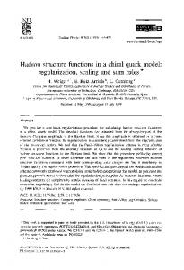
Figure 1: Comparison of the pion valence distribution,uπvalence (x), result from the valon −

model calculation (solid line), SMRS, Ref. [13] (dashed line), GRS, Ref. [14] (dotted line), and the data from E615 [2] at Q2 = 25GeV 2 .

pion as: Z

1

x x dy G U (y)q sea ( , Q2 ) + U y π+ y

Z

1

x x dy G D¯ (y)q sea ( , Q2 ) ¯ D + y y π x x (11) Evaluation of these convoluted integrals requires us to determine G valon (y) π or, alternatively, finding µm and νm . Since the two valons in the pion, apart from flavor, cannot be distinguished and since the masses of the U ¯ valons are the same, therefore their average momentum also must and D be the same. This can be achieved only if µm = νm , leaving us with only one parameter. We use the valence distribution data in π − at Q2 = 25 GeV 2 from the Drell-Yan experiment of E615 collaboration [2] to find this parameter. The fit to the data of Ref. [2] is shown in Fig. (1), which is obtained by taking the starting scale,Q20 = 0.47 GeV 2 with ΛQCD = 0.22 GeV. The goodness of the fit is checked by χ2 minimization procedure. We find that the χ2 per degree of freedom is 1.2 and that µm = νm = 0.01. As a comparison, in Fig.(1) we have also shown the results from the determination of [13] as dashed line and those of [14] as dotted line, both at Q2 = 25 GeV 2 . In fitting the data we have also allowed both ΛQCD and Q20 to be free parameters and obtained an equally good description of the data with Q20 = 0.35 GeV 2 and ΛQCD = 0.175 GeV resulting in µm = νm = 0.03. However, it seems that ΛQCD = 0.175 is too low for four active flavor. As such, we choose the former against the latter. With the Determination of these parameters, it is important to check the valence quark sum rule in π+ xqsea (x, Q2 )

=

5

valon (z = x/y, Q2 ), from pion. Using the explicit form of Eq. (2), i.e. zqvalence the appendix of Ref. [11], we find that each of the integrals in Eqs. (710) gives 0.9994, 1.002, and 1.008 at Q2 = 3, 10, 20 GeV 2 , respectively; an excellent confirmation of the valence quark sum rule. The first two moments of pion valence quark distribution is also calculated at Q2 = 49 GeV 2 for the purpose of comparison with the findings of Ref. [13]. We find that 2 < xq valence >= 0.378 and 2 < x2 q valence >= 0.151. This is to be compared π π with 0.40 ± 02 and 0.16 ± 0.01 of Ref. [13], respectively. From Eq. (5) we can infer some knowledge about the charge and matter distributions of the pion [8]. The longitudinal momentum space is related to the coordinate space by a Fourier Transform and a boost to infinitemomentum frame. Since the valon structure originates from QCD virtual processes, which are flavor independent, the matter and the charge densities in the valon ought to be flavor independent. Hence, the charge density in, say, π + is 1 2 (12) ρq (y) = G U (y) + G D¯ (y), 3 π+ 3 π+ whereas for the matter density distribution we assume that it is proportional to the total valon distribution, i.e. ,

ρm (y) =

1 (G U (y) + G D¯ (y)). 2 π+ π+

(13)

The integral of both quantities in Eqs.(12) and (13) are equal to one. Let us write the explicit form of G valon : π+

G

U π+

=G

¯ D π+

= 1.020(1 − y)0.01 y 0.01 .

(14)

It is evident that this function is very broad in momentum space. This feature is expected, for, it indicates that the valons are tightly bound. This is also a reflection that the pion is much lighter than the mass of its constituent quarks. The parameters, µm and νm obtained here are slightly different from those used in Ref. [4,11,12] and are significantly different from those quoted in [15]. In [4,11] the values µm = 0.01 and νm = 0.06 were used, while the determination of Ref. [12] is µm = νm = 0, thus, there is no significant differences among this work and those of Ref.[4,11,12]. In Ref. [15] the pion cloud model in conjunction with the valon model is used to calculate the pion structure. They find that µm = 0.044 and νm = 0.372. In this work and in Ref. [4] the parton distribution in a valon is derived from 6

QCD alone, with no phenomenological assumption. However, in Ref. [4], the focus was on the low x behavior of the pion structure function, whereas here we have used data at rather large x (x > 0.2) region to determine the valon distribution in the pion. In Fig. (2) we present the full pion structure function at Q2 = 7 and Q2 = 15 GeV 2 at small x, (x = [10−4 , 10−2 ]), region and compared the results with those obtained from Sutton,et al. [13] and Gluck, Reya, and Schienbein [14] parameterizations. In Fig. (2) two sets of data points are shown, which correspond to the two different methods of normalization used by ZEUS collaboration.While the results from Ref. [14] agrees with the additive quark model normalization, the parameterization of Ref. [13] is qualitatively closer to the effective one-pion-exchange model normalization. Note that although the parameterization of Ref.[14] provides a good description of the additive quark model normalization of the data, it fails to describe the large x data of Ref. [2] as is apparent from Fig. (1). As can be seen from the figure, the valon model results are in good agreement with the pion flux normalization of the data. It is also interesting to note that in the valon model a simple relationship holds rather well between proton and pion structure functions, namely, F2π = kF2p , with k ≃ 0.37 [4]. This observation has also been made by the ZEUS Collaboration [3]. The ZEUS group will soon release two new measurement: one is photoproduction study from which the pion trajectory can be determined; and the second is a measure of the exponential Pt slopes in deep inelastic scattering that can be used to limit the choice for the form factor F (t) [16]. These measurements should help to resolve the normalization issue.

3.2

B. Kaon

The treatment of the kaon structure function is similar to that of pion, except that we need to determine valon distribution in the kaon. We will concentrate on K − , since there are some data [17] which provide information about the valence distribution in K − . In Refs. [8, 11, 12] it is stated that the general form of the exclusive valon distribution in a meson is as follows GV1 V2 (y1 , y2 ) = [β(µk + 1, νk + 1)]−1 y1µk y2νk δ(y1 + y2 − 1)

(15)

Integrating over either of yi will give the individual valon distribution in the meson, as in Eq. (5). So, we can write a similar equation for the valon distributions in K − , except that µm and νm are different and we label them as µk and νk , respectively. One way to determine these parameters is fitting G valon (y) to some experimental data. Unfortunately, there is hadron

7

Fpion 2

Fpion 2 1.4

1

1.2 0.8

1 0.8

0.6

0.6 0.4

0.4 0.2

0.2 0.001

0.002

0.003

0.004

0.005

0.006

0.007

x

0.005

0.01

0.015

0.02

Figure 2: Pion structure function at Q2 = 7GeV 2 (Left) and at Q2 = 15GeV 2 (Right). The diamonds and squares are pion flux and additive quark model normalization of the data [3], respectively. The solid line represents the calculated results from the valon model. The bdashed line is the result from SMRS [13] and the dotted line corresponds to GRS [14]determination.

no experimental data on the valon distribution of any hadron, and from the theoretical point of view, the function G valon (y) cannot be evaluated hadron accurately. However, there are some limited data on the ratio R=

x¯ uk− x¯ uπ−

(16)

at large x values [17], and can be used to fit equations of the form (7-10) to get µk and νk . Maintaining the same values for Q20 and Λ as in the case of pion, we have fit the data of Ref. [17] and obtained µk = 0.13 and νk = 0.28 with a χ2 = 0.646 per degrees of freedom. The fit is shown in Fig. (3). In our fit to this data set, both valence and sea u ¯ are included, although the data points are at rather large x and hence, the sea quark contribution to R is marginal. In the alternative, we can be guided by making a simple phenomenological assumption as follows [12]. Since K − consists of two valons with different masses. It is obvious from Eq. (15) that the average momentum fractions of the light valon, y¯1 and the heavy valon, y¯2 , are y¯1 = (µk +1)/(µk +νk ) and y¯2 = (νk +1)/(µk +νk ), respectively. Thus, letting the ratio of the momenta be equal to ratios of their masses, we get µk + 1 mU 300 y¯1 = = 0.6 (17) = ≃ y¯2 mS 500 νk + 1 In this way νk is restricted by νk = (µk + 0.4)/0.6, 8

(18)

x

R 1 0.8 0.6 0.4 0.2

0.2

0.4

0.6

0.8

1

x

Figure 3: The ratio R as a function of x as measured by [17]. The curve is obtained from the model by fitting the data at Q2 = 25 GeV 2 . R 2

1.5

1

0.5

0.2

0.4

0.6

0.8

1

x

Figure 4: The ratio R as a function of x as measured by [17]. the curve is obtained with µk = −0.35 at Q2 = 25 GeV 2 . hence, leaving us with only one parameter, µk , to be determined. A one parameter fit to the data of Ref. [17] is highly unsatisfactory, with µk = −0.35 as can be seen in Fig. (4). Authors of Ref. [12] have used inclusive distribution of K + → π + and K + → π − and found µk = 1 and νk = 2 which also do not support the data of Ref. [17]. An earlier QCD calculation [18] of the ratio, which takes into account the difference in quark mass, however agrees with the data. Nevertheless, it seems that R being around 0.5 at x = 0.95 is too high. Considering the large error bars in the data, the accuracy of the data, at least, at large x is suspect. One possible way of determining the valence quark density in kaon would be the difference of two cross sections in K + p → µ+ µ− + X and K − p → µ+ µ− + X processes. While the determination of the valon distribution in kaon remains uncertain, we will proceed with the values obtained for µk and µk without the 9

xUvalence 0.3 0.25 0.2 0.15 0.1 0.05 0.2

0.4

0.6

0.8

1

x

Figure 5: The valence quark distribution, x¯u(x), in π − (solid curve) and in K − (dashed curve) . The curves are obtained from the model at Q2 = 25 GeV 2 .

restriction of Eq. (18), namely, µk = 0.13 and νk = 0.28 and arrive at the following valon distributions in K − ; GkS (y) = 1.4768y 0.28 (1 − y)0.13 (19) ¯ With these relations the average momentum fraction carried by U and S valons are 0.469 and 0.531, respectively. Using these valon distributions along with Eqs. (7-10) for K − , the valence quark distributions for π − and k− are calculated at Q2 = 25GeV 2 and shown in Fig.(5). It should be noted that in Drell-Yan processes, obtaining experimental information on the strange valence and sea quark distribution in kaon is not practical. Because those components in kaon only contribute to the total cross section of the Drell-Yan processes through valence-sea and s − s¯ annihilation and these contributions being small makes it difficult to separate them. The valon model, on the other hand, provides valuable information about these components. Figures (6) shows the strange valence and sea quark distributions in K − . Both are calculated at Q2 = 25 GeV 2 from the model. For the purpose of comparison, in Figure (7) we show sea quark distributions in a valon. The sea quark distribution is calculated originally for u and d type partons. The strange sea quark distributions are generally ¯ ∼ smaller than the light sea quark distributions so that in proton 2¯ s/(¯ u + d) −4 0.5[19] Nevertheless, by the time x ∼ 10 s¯ ≈ u ¯. GkU¯ (y) = 1.4768y 0.13 (1 − y)0.28 ,

−

−

10

xSsea 0.14

xSvalence 0.3

0.12

0.25

0.1

0.2

0.08

0.15

0.06

0.1

0.04

0.05

0.02

0.2

0.4

0.6

0.8

1

x 0.2

0.4

0.6

0.8

Figure 6: Strange quark distribution in K − at . Q2 = 25 GeV 2 . Left figure is the valence component and the right figure is that of strange sea distribution.

z qsea 0.25

0.2

0.15

0.1

0.05

0.2

0.4

0.6

0.8

z

Figure 7: Sea parton distributions in a valon at Q2 = 25 GeV 2 .

11

1

x

4

Conclusion

We have used the notion of the valon model to determine the structure of mesons. Since the partonic structure of a valon is already known, the structure function of any meson needs only two parameters to be completely determined. The valon model provides information about the sea quark distribution of mesons that are out of reach experimentally. While the pion structure is determined fairly accurately, the structure of kaon remains uncertain, due to the lack of accurate data or incompatibility of data sets from different experiments.

References [1] J. Badier et al., Z. Phys. C 18, 281. (1983); J. Badier et al., Phys. Lett. B 93,(1980) 354; M. Bonesini et al., Z. Phys. C 37, 538 (1988). [2] J. S. Conway et al., Phys. Rev. D 39, 92 (1989). [3] ZEUS Collaboration, S. Chekanov et al., Nucl. Phys B 637 (2002) 3. [4] Firooz Arash, Phys. Lett. B 557 (2003) 38. [5] M. Osipenko et al., Phys. Rev. D 67(2003) 092001; hep-ph/0301204. [6] R. Petronzio, S. Simula, and G. Ricco, hep-ph/0301206. [7] G. Altarelli, N. Cabibo, L. Maiani, and R. Petronzio, Nucl. Phys. B69, 531 (1974). [8] R. C. Hwa, M. S. Zahir, Phys. Rev. D 23, 2539 (1981); R. C. Hwa, Phys. ReV. D 22 (1980) 1593. [9] M. Lavelle, D. McMullan, Phys. Lett. B 371 (1996) 83. [10] M. Lavelle, D. McMullan, Phys. Rep. 279 (1997) 1. [11] Firooz Arash, Ali N. Khorramian, Phys. Rev. C 67 045201 (2003). [12] Rudolph C. Hwa and C. B. Yang, Phys. Rev. C 66, 025205 (2002). [13] P.J. Sutton, A.D. Martin, R. G. Roberts, and W. J. Stirling, Phys. Rev. D 45, 2349 (1992).

12

[14] M. Gluck, E. Reya, I. Schienbein, Eur. Phys. J. C 10, 313-317 (1999). [15] C. Avila, J. C. Sanabria, and J. Magnin, Phys. ReV. D 67 (2003) 054020; hep-ph/0210421. [16] M. Derrick, ZEUS Coll., Private Communication. [17] Klause Freudenreich, Int. Jour. Mod. Phys. A 5 (1990) 3643; Alos, see the second paper in Ref. [1]. [18] F. Martin et al., XV th Recontre de Moriond (1980). [19] H. Abramowicz et al. (CDHSW Coll.), Z. Phys. C15 (1982)19; Z. Phys. C17(1983) 283; K. Lang et al. (CCFR Coll.), Z. Phys. C33(1987)483; C. Foudas et al. (CCFR Coll.), Phys. Rev. Lett. 64 (1990) 1207.

13