Mesozooplankton structure and functioning during the onset of ... - Core

Mesozooplankton structure and functioning during the onset of the Kerguelen phytoplankton bloom during the KEOPS2 survey F Carlotti, M.-P Jouandet, A Nowaczyk, M Harmelin-Vivien, D Lefèvre, P Richard, Y Zhu, M Zhou

To cite this version: F Carlotti, M.-P Jouandet, A Nowaczyk, M Harmelin-Vivien, D Lefèvre, et al.. Mesozooplankton structure and functioning during the onset of the Kerguelen phytoplankton bloom during the KEOPS2 survey. Biogeosciences, European Geosciences Union, 2015, 12, pp.4543-4563. .

HAL Id: hal-01231387 https://hal-amu.archives-ouvertes.fr/hal-01231387 Submitted on 20 Nov 2015

HAL is a multi-disciplinary open access archive for the deposit and dissemination of scientific research documents, whether they are published or not. The documents may come from teaching and research institutions in France or abroad, or from public or private research centers.

L’archive ouverte pluridisciplinaire HAL, est destinée au dépôt et à la diffusion de documents scientifiques de niveau recherche, publiés ou non, émanant des établissements d’enseignement et de recherche fran¸cais ou étrangers, des laboratoires publics ou privés.

Biogeosciences, 12, 4543–4563, 2015 www.biogeosciences.net/12/4543/2015/ doi:10.5194/bg-12-4543-2015 © Author(s) 2015. CC Attribution 3.0 License.

Mesozooplankton structure and functioning during the onset of the Kerguelen phytoplankton bloom during the KEOPS2 survey F. Carlotti1,4 , M.-P. Jouandet1,4 , A. Nowaczyk1,4 , M. Harmelin-Vivien1,4 , D. Lefèvre1,4 , P. Richard2 , Y. Zhu1,3,4 , and M. Zhou1,3,4 1 Aix

Marseille Université, CNRS/INSU, IRD, Mediterranean Institute of Oceanography (MIO), UM 110, Marseille, France Environnement et Sociétés, UMR 7266 CNRS-Université de La Rochelle, 2 Rue Olympe de Gouges, 17000 La Rochelle, France 3 Department of Environmental, Earth and Ocean Sciences, University of Massachusetts Boston, Boston, MA 02125, USA 4 Université du Sud Toulon-Var, CNRS/INSU, IRD, Mediterranean Institute of Oceanography (MIO), UM 110, La Garde, France 2 Littoral

Correspondence to: F. Carlotti ([email protected]) Received: 28 November 2014 – Published in Biogeosciences Discuss.: 04 February 2015 Revised: 03 June 2015 – Accepted: 14 June 2015 – Published: 31 July 2015

Abstract. This paper presents results on the spatial and temporal distribution patterns of mesozooplankton in the naturally fertilized region to the east of the Kerguelen Islands (Southern Ocean) visited at early bloom stage during the KEOPS2 survey (15 October to 20 November 2011). The aim of this study was to compare the zooplankton response in contrasted environments localized over the Kerguelen Plateau in waters of the east shelf and shelf edge and in productive oceanic deep waters characterized by conditions of complex circulation and rapidly changing phytoplankton biomass. The mesozooplankton community responded to the spring bloom earlier on the plateau than in the oceanic waters, where complex mesoscale circulation stimulated initial more or less ephemeral blooms before a broader bloom extension. Taxonomic compositions showed a high degree of similarity across the whole region, and the populations initially responded to spring bloom with a large production of larval forms increasing abundances, without biomass changes. Taxonomic composition and stable isotope ratios of sizefractionated zooplankton indicated the strong domination of herbivores, and the total zooplankton biomass values over the survey presented a significant correlation with the integrated chlorophyll concentrations in the mixed layer. The biomass stocks observed at the beginning of the KEOPS2 cruise were around 1.7 g C m−2 above the plateau and 1.2 g C m−2 in oceanic waters. Zooplankton biomass

in oceanic waters remained on average below 2 g C m−2 over the study period, except for one station in the Polar Front zone (F-L), whereas zooplankton biomasses were around 4 g C m−2 on the plateau at the end of the survey. The most remarkable feature during the sampling period was the stronger increase in abundance in the oceanic waters (25 × 103 to 160 × 103 ind m−2 ) than on the plateau (25 × 103 to 90 × 103 ind m−2 ). The size structure and taxonomic distribution patterns revealed a cumulative contribution of various larval stages of dominant copepods and euphausiids particularly in the oceanic waters, with clearly identifiable stages of progress during a Lagrangian time series survey. The reproduction and early stage development of dominant species were sustained by mesoscale-related initial ephemeral blooms in oceanic waters, but growth was still food-limited and zooplankton biomass stagnated. In contrast, zooplankton abundance and biomass on the shelf were both in a growing phase, at slightly different rates, due to growth under sub-optimal conditions. Combined with our observations during the KEOPS1 survey (January–February 2005), the present results deliver a consistent understanding of patterns in mesozooplankton abundance and biomass from early spring to summer in the poorly documented oceanic region east of the Kerguelen Islands.

Published by Copernicus Publications on behalf of the European Geosciences Union.

4544 1

Introduction

The eastern part of the Kerguelen Plateau sustains one of the most important local foraging areas for land-based marine predators (birds, penguins, seals and elephant seals) and for whales (Hindell et al., 2011; Blain et al., 2013). Satellitebased chlorophyll images of this region highlight the intensive seasonal Kerguelen bloom and its south-east extension off the archipelago (Schlitzer, 2002; Thomalla et al., 2011; Blain et al., 2013; Trull et al., 2015). During the KEOPS1 survey (KErguelen Ocean and Plateau compared Study), the origin and fate of the elevated phytoplankton biomass over the Kerguelen Plateau were addressed (Blain et al., 2008), with a focus on the mechanisms supplying the surface waters with iron. The Kerguelen Plateau, oriented along the 70◦ E meridian, forms a large north-west/south-east topographical barrier of the Antarctic Circumpolar Current, forcing the Polar Front (PF) to pass above the plateau south of the Kerguelen Islands in a meandering course (Fig. 1). The PF flow on the shelf induces entrainment and mixing of Feenriched shelf waters from plateau sediments in the oceanic upper layer in the area east of Kerguelen, and is a driver of relatively high phytoplankton bloom concentrations, with a strong increase from October to December (Blain et al., 2007, 2013), initially dominated by diatoms of high growth rates (Quéguiner, 2013) contrasting with the generally highnutrient low-chlorophyll (HNLC) surface oceanic waters of the Southern Ocean. This enhanced biological productivity in the eastern area fuels the trophic level of zooplankton and micronekton, which are potential prey of fish and squid forage required to meet the demand of top predators. During the KEOPS1 cruise (January–February 2005), the mesozooplankton populations, mainly copepods, were already well established without significant spatial and temporal changes in species composition and biomass, around 10.6 g C m−2 above the plateau and around 5 g C m−2 in HNLC oceanic waters (Carlotti et al., 2008). The KEOPS1 survey occurred during the decline phase of a natural long-term spring bloom initiated in November. How the zooplankton populations increase from overwinter stocks by exploiting new primary production in early spring is still poorly documented because descriptions of seasonal variations of mesozooplankton standing stocks in oceanic Antarctic regions are scarce. The implementation of the Southern Ocean CPR survey delivers consistent information regarding the seasonal succession of zooplanktonic communities in the Southern Ocean south of Australia (Hosie et al., 2003; Hunt and Hosie, 2006a, b). In the PF zone, a relatively strong increase in zooplankton abundance occurs in spring, from October to November (see Hosie et al., 2003, their Fig. 3), mainly due to changes in density of all common taxa from average winter levels still maintained until October (Hunt and Hosie, 2006b). The largest copepods of the region (Rhincalanus gigas, Calanoides acutus, Ctenocalanus citer) are seasonal migrators which arrive in the surface layer Biogeosciences, 12, 4543–4563, 2015

F. Carlotti et al.: Mesozooplankton structure and functioning from winter diapause depths when Chl a concentrations increase (October to November). Overwintering females may spawn reserves even before the full bloom, whereas overwintering stages other than adult stages resume their growth in surface water up to mature adults which produce new cohorts during the full bloom period (Atkinson, 1998; Hunt and Hosie, 2006b). Other smaller species (Calanus similimus, Oithona sp., etc.) resume their population development from survivors from the previous year and start reproduction earlier in spring (Atkinson, 1998). There are no historical CPR data around the Kerguelen Islands, but some pieces of the puzzle suggest similar patterns. Zooplankton distribution patterns observed by Semelkina (1993) during the SKALP cruises around the Kerguelen Islands (46–52◦ S, 64–73◦ E) from February 1997 to February 1998 showed a change in biomass (fourfold higher) from winter (July–August) to midsummer (February), but did not describe this early spring period. It is also worth noting that the seasonal zooplankton abundances recorded from February 1992 to January 1995 at the KERFIX station, located around 60 miles south-west of the Kerguelen Islands in 1700 m of water, show a major increase in copepod densities from September to January (Razouls et al., 1998). The main objective of the KEOPS2 study was to investigate the early phase (October–November 2011) of the seasonal marine productivity in this Kerguelen region in order to gain new insights into the biogeochemistry and ecosystem response to iron fertilization. The study was conducted in contrasted environments differently impacted by iron availability, i.e. on the plateau waters, in areas common with KEOPS1, and in productive oceanic deep waters with strong mesoscale activity to the east of the Kerguelen Islands. The focus of the present paper is to document the responses of zooplankton in terms of species diversity, density and biomass in the mosaic of blooms observed during the survey, and to characterize the trophic pathways from primary production to large mesozooplanktonic organisms.

2 2.1

Material and methods Study site and sampling strategy

The KEOPS2 survey was performed east of the Kerguelen Islands in the Indian sector of the Southern Ocean, on board R.V. Marion Dufresne, between the 15 October and the 20 November 2011. It firstly consisted of predefined stations along two transects (Fig. 1) the first oriented north– south between 46◦ 50 and 49◦ 08 S, and subsequently referred to as the TNS transect (stations TNS1 to TNS10, blue dots in Fig. 1), and the second oriented east-west between 69◦ 50 and 74◦ 60 E, referred to as the TEW transect (stations TEW1 to TEW8, green dots on Fig. 1). Along these two transects, zooplankton samples were collected once at each station. The TEW transect crossed the Polar Front (PF) twice, first bewww.biogeosciences.net/12/4543/2015/

F. Carlotti et al.: Mesozooplankton structure and functioning

4545

70°E

72°E TNS-1

40°S

200 m

50°S 60°S

Kerguelen I. R-2

Polar Front

TNS-2

TNS-3 TNS-4 TEW-5 TEW-3 TEW-2 TNS-7 TEW-1 TNS-8 TNS-9 TNS-10 A3-1 / A3-2

TEW-7 TEW-8 F-L TNS-4 E-5 TNS-5 TEW-5 TEW-4 E-2 E-1 E-4E E-3 E-4W TNS-6

TEW-6

Figure 1. Map of the KEOPS2 study area and station locations. The locations of the stations are marked by coloured dots. The southern station A3 (red dot) was visited twice at the beginning (station A3-1) and the end (station A3-2) of the KEOPS2 survey. This station, A3, situated in the middle of the shelf, was the reference station for the shelf bloom observed during KEOP1. The stations of the north–south transect (shown by blue dots) are located in oceanic waters and were sampled just after the first visit to A3, from south to north (stations TNS1 to TNS10), from the central plateau (TNS10) across the recirculation feature (TNS7 toTNS3) and the Polar Front (TNS3, TNS2) and into subantarctic waters (TNS1). Station R-2 (black dot) in the west of the Kerguelen Plateau represented a HNLC reference station. The TEW transect (east–west transect) was sampled from west to east from the near coast of Kerguelen Island (TEW1) above the shelf (TEW32) and shelf break (TEW3) across the middle of the recirculation system (TEW4 to TEW6), and beyond the southward meandering Polar Front (TEW7 and TEW8) in the extreme east of the study region. The survey ended with a quasi-Lagrangian time series (stations E1–E5 in orange dots in the zoom panel), during a progressive phase of the bloom within the recirculation system in the meander of the Polar Front. In addition, one station (station F-L) situated in high-biomass waters in the extreme north-east of the study region, near the downstream location of the PF, was sampled within the period of the time series.

tween TEW3 and TEW4 where the southern branch of the PF flows northwards along the shelf break, and secondly between TEW6 and TEW7, where the PF is directed southwards after a semicircle trajectory maintaining a large stationary meander in this area. The most westerly stations were located over the inner (TEW1) and outer (TEW2) parts of the Kerguelen shelf. The most easterly stations (TEW7 and TEW8) were situated in Subantarctic Mode Water whereas the central section (TEW4 to TEW6) within the stationary meander was covered by mixed Antarctic surface water (Farías et al., 2015; Trull et al., 2015). In addition, intensive sampling (24 h) was performed at nine strategic stations (Fig. 1) located in the eastern bloom in the Polar Front zone (F-L station), in the north-eastern bloom (set of E stations), in the south-eastern bloom above the Kerguelen Plateau (A3 station) and in the deep waters southwest of the Kerguelen Islands considered as a HNLC reference station (R station). Station A3 (common with KEOPS1) was sampled twice during KEOPS2: at the winter (A3-1) stage and the spring stage (A3-2). The patterns of change over time of the north-eastern bloom, located in a complex recirculation area inside the stationary meander of the Polar Front (Park et al., 2014; Zhou et al., 2014), was studied by a quasi-Lagrangian survey including five stations (E1-E2-E3E4E-E5). Real-time-satellite images (chlorophyll and altimetry) in combination with trajectories of 50 drifters released during the first part of the cruise were used to carefully decide the

www.biogeosciences.net/12/4543/2015/

positions of these five stations (Trull et al., 2015, their Fig. 2). In addition, we visited a productive station (E4W, red dot in Fig. 1) located in the plume of chlorophyll observed downstream of the plateau and close to the jet induced by the PF. 2.2

Mesozooplankton sampling

Zooplankton collection was conducted at 27 stations with a double Bongo (60 cm mouth diameter) with one 330 µm mesh net and a 120 µm mesh net mounted with filtering cod ends. Hauls were done from a 250 m depth to the surface at 0.5 ms−1 . The stations of the TNS transect (stations TNS 1 to TNS10) and the stations of the TEW transect (stations TEW1 to TEW8) were each sampled once. During the intensive stations study (including A3 – which was visited twice – R2, F-L, and the set of E stations), zooplankton samples were taken twice daily, by day and by night (stations were named R2-d and R2-n, for instance). For each sampling station, two successive net hauls at each station were done: the first net haul was taken for ZOOSCAN processing, taxonomy study and dry weight measurements, and a second net haul was taken for isotope analysis. The cod-end contents of the first haul were kept fresh and split into two parts with a Motoda box (Motoda, 1959). The first part was preserved in 4 % borax-buffered formalin seawater for further laboratory study of zooplankton community structure (taxonomy, abundance and size structure) and for biomass estimates from organism biovolume (see beBiogeosciences, 12, 4543–4563, 2015

4546


low). The second half of the sample was preserved for dry weight measurements. As many of the 120 µm size nets were clogged with phytoplankton cells and aggregates, we could not finally use the sample for dry weight measurements and ZOOSCAN processing. However we used the 120 µm mesh net samples for isotope analysis (as described in the following paragraph). To prepare samples for isotope analysis, size fractions were obtained as follows. Samples from the second 330 µm net haul at each station were passed sequentially through five sieves arranged in a column (2000, 1000, 500, 200 and 80 µm meshes). The three largest sizes were then collected, and for the largest size (2000 µm) large organisms such as salps and euphausiids were separated into additional containers. To provide more material for the two smallest sizes (200, 80 µm), these materials were retained on the sieves and the contents of the 120 µm net haul were passed through the entire set of five sieves (with the overlying 2000, 1000 and 500 µm sieves serving to block larger organisms and aggregates, but without those materials being collected). All samples were placed in small containers and immediately deepfrozen (−80 ◦ C). 2.3

ing set of images. The biovolume (BV; mm3 ) was calculated from the organism image areas and morphometric parameters. In order to estimate the biomass of each organism, we used the same conversion as in Carlotti et al. (2008); each measured biovolume (BV; mm3 ) of a zooplankton individual was converted into biomass (W , in units of mg dry weight, DW) using the following relationship: log (W ) = 0.865 log (BV) − 0.887 (Riandey et al., 2005). Carbon content was assumed to be 50 % of body dry weight. In this article, the terms “ZOOSCAN abundance” and “ZOOSCAN biomass” will designate the values derived from the laboratory ZOOSCAN processing. The abundance and biomass of organisms were then grouped into four size fractions (< 500, 500–1000, 1000–2000 and > 2000 µm) based on their ECD, and summed to deliver the total abundance and biomass per sample over the upper 250 m. The choice of the net haul sampling depth was based on mixed layer depth found at the first station of the cruise, and maintained afterwards. Abundance and biomass values are normalized to the volume of water filtered in situ. An ANOVA test (5 % significance level) was used to test differences of abundance and biomass between stations or oceanic areas.

Abundance and biomass using the Zooscan 2.4

For each station, the cod-end content of a 330 µm mesh size net was processed using ZOOSCAN (www.zooscan. com) to determine the zooplankton community size structure. ZOOSCAN has recently been used to study the zooplankton community in various areas and has been validated by comparisons with traditional sampling methods (Grosjean et al., 2004; Schultes and Lopes, 2009; Gorsky et al., 2010). Our ZOOSCAN setup is similar to the one described by Gorsky et al. (2010), and our sample processing protocol is fully presented in Nowaczyk et al. (2011), following the recommendations of Gorsky et al. (2010). After homogenization, each sample was quantitatively split with a Motoda box once back in the laboratory and a fraction of each preserved sample containing a minimum of 1000 particles (in general 1/32 or 1/64 of the whole sample) was placed on the glass plate of the ZOOSCAN. Organisms were carefully separated one by one manually with a long wooden needle, in order to avoid overlapping. Each image was then run through the ZooProcess plug-in using the image analysis software Image J (Grosjean et al., 2004; Gorsky et al., 2010). Several measurements of each organism were then computerized. Organism size is given by its equivalent circular diameter (ECD) and can then be converted into biovolume, assuming each organism is an ellipsoid (more details in Grosjean et al., 2004). The lowest ECD detectable by this scanning device is 300 µm. To discriminate between aggregates and organisms, we used a training set of about 1000 objects which were selected automatically from 40 different scans. This protocol allows discrimination between aggregates and organisms by building the initial trainBiogeosciences, 12, 4543–4563, 2015

Taxonomic determination

Common taxa were counted with the binocular microscope for taxonomy. For the 330 µm mesh size net, around 600 organisms were counted from subsamples 1/32 or 1/64). For the 120 µm mesh size net, around 400 organisms were counted from diluted samples (dilution from one to ten thousandths). The whole sample was examined for either rare species and/or large organisms (i.e. euphausiids, amphipods). Identification of the copepod community was done down to species level and groups of developmental stage when possible. Species/genus identification was done according to Rose (1933), Tregouboff and Rose (1957) and Razouls et al. (2014). Organisms other than copepods as well as meroplankton were identified down to taxa levels. Identifications were done to genus level for copepods, amphipods, pelagic molluscs, polychaetes, Thaliacea and Cnidarians; and to taxa level for other major holoplanktonic and meroplanktonic groups. To identify which taxonomic groups contribute to the four size fractions defined from ZOOSCAN measurements done on the 330 µm mesh net samples (see above), each observed organism was classified as small, medium, large or very large mesozooplankton, which approximately corresponds to the four size fractions determined by ZOOSCAN (see above). Similarly, the organisms observed and counted from the 120 µm mesh size net samples were also classified into small and medium size fractions. Distribution in larger size fractions was not considered from the 120 µm mesh size net samples, the large organisms being undersampled.



4547

Figure 2. Integrated 0–200 m mesozooplankton abundance counted from ZOOSCAN for the different stations sampled during KEOPS2 with size-fraction distributions. Size fractions: < 500 µm, black; 500–1000 µm, dark grey; 1000–2000 µm, light grey; > 2000 µm, white.

2.5

Biomass measurement

The subsample of the 330 µm mesh net for bulk biomass measurement was filtered onto a pre-weighed and precombusted GF/F filter (47 mm) which was quickly rinsed with distilled water and dried in an oven at 60 ◦ C for 3 days on board. The dry weight (mg) of 19 samples was calculated from the difference between the final weight and the weight of the filter, and biomass (mg DW m−2 ) was extrapolated from the total volume sampled by the net. 2.6

Stable isotope analysis

Before processing, identification of the broad taxonomic composition of each sample preserved for isotopic measurements was performed under a binocular microscope. When possible, the main group of organisms in the largest > 2000 µm size fraction were sorted out and processed separately. Then, zooplankton fractions were freeze-dried and ground into a homogeneous powder. As they may contain carbonates, an acidification step was necessary to remove 13 C-enriched carbonates (DeNiro and Epstein, 1978; Søreide et al., 2006). A subsample was acidified with 1 % HCl, rinsed, dried and used for determination of δ 13 C values, while the other untreated subsample was used for determination of nitrogen isotopic composition. Three replicates were performed on each plankton fraction per sampled station for both δ 13 C and δ 15 N values. Stable isotope measurements were performed with a continuous-flow isotope-ratio mass spectrometer (Delta V Advantage, Thermo Scientific, www.biogeosciences.net/12/4543/2015/

Bremen, Germany) coupled to an elemental analyzer (Flash EA1112 Thermo Scientific, Milan, Italy). Results are expressed in parts per thousand (‰) relative to Vienna Pee Dee Belemnite and atmospheric N2 for δ 13 C and δ 15 N, respectively, according to the equation: δX = [(Rsample /Rstandard )− 1] ×103 , where X is 13 C or 15 N, and R is the isotope ratio 13 C / 12 C or 15 N / 14 N, respectively. Calibration was performed using certified reference materials (USGS-24, IAEACH6, -600 for carbon; IAEA-N2, -NO-3, -600 for nitrogen). Analytical precision based on repeated analyses of acetanilide (Thermo Scientific) used as an internal standard was < 0.15 ‰. Percentage of organic C and organic N were obtained using the elemental analyzer and were used to calculate sample C / N ratios. Lipids are depleted in δ 13 C relative to proteins and carbohydrates, and variation in lipid content between organisms can introduce considerable bias into carbon-stable isotope analyses (Bodin et al., 2007; Post et al., 2007). Like most polar marine organisms (Lee et al., 2006), KEOPS2 zooplankton fractions could present a high lipid content (up to 20 % dry mass, data not shown), reflected by high C / N values. Thus, δ 13 C acidified sample values of fractions > 200 µm were corrected according to the formula calculated by Post et al. (2007) for aquatic organisms, using the C / N ratio of each sample: δ 13 Cnormalized = δ 13 Cacidified – 3.32 + 0.99 × C / N Acidified δ 13 C values of the lowest size fraction (80– 200 µm) were not lipid-corrected due to their low lipid content (< 5 %, data not shown). The resulting δ 13 Cnormalized provides an estimate of δ 13 C corrected for the effects of

Biogeosciences, 12, 4543–4563, 2015

4548


lipid concentration. Lipid correction calculated by Smyntek et al. (2007) for zooplankton give δ 13 C values 0.63 ± 0.01 ‰ lower than those of Post et al. (2007). As δ 13 C values provided by Trull et al. (2015) were not lipid-normalized, acidified δ 13 C values for all zooplankton size fractions are indicated in Table 2, along with lipid-normalized δ 13 C values, to allow comparisons between the two data sets. To consider the relationships between zooplankton and phytoplankton, we used the groups of stations (T-groups) defined by Trull et al. (2015) based on chemometric measurements of phytoplankton. The HNLC reference station R2 belonged to T-group 1, along with station TEW4. Stations located on the plateau (A3 and E4) and in the eddy (E1 to E5) are included in T-group 2 and T-group 3, respectively. The two most easterly stations, located in the open ocean near the Polar Front (F-L and TEW8), belonged to T-group 5. Trull’s T-group 4 corresponded to coastal stations not sampled for zooplankton analysis. 2.7

Data analysis

The effect of stations and dates (n = 12) on zooplankton abundance and biomass was tested statistically using oneway ANOVA with the statistical software Statistica v7. The statistical significance was tested at the 95 % confidence level. Community patterns for taxa abundance were explored using the Primer (V6) software package which has been shown to reveal patterns in zooplankton communities (e.g. Clarke and Warwick, 2001; Wishner et al., 2008). Data sets were power-transformed (fourth root), and the Bray–Curtis dissimilarity index between stations (Bray and Curtis, 1957) was calculated employing all taxonomic categories that contributed at least 1 % to any sample in that data set. Different groups of zooplankton (BC groups) were individualized based on their taxonomic composition. Mean C- and Nstable isotope values among size fractions and between day and night within each fraction were compared by one-way ANOVAs followed by Tukey post-hoc tests, after testing for normality by a Levene test. 3 3.1

Results Hydrology and trophic conditions

The KEOPS2 campaign was characterized by conditions of complex circulation and rapidly changing phytoplankton biomass (see Trull et al., 2015, their Figs. 1 and 2 and Suppl.). During the survey, the horizontal circulation pattern was dominated by the northernmost branch of the PF (Park et al., 2014) flowing across the plateau in the narrow, middepth (1000 m) channel just to the south of Kerguelen Island (Fig. 1). After passing to the east of the plateau, the jet flows outside the shelfbreak northwards and enters in a bathymetrically trapped cyclonic recirculation system (d’Ovidio et al., 2015; Park et al., 2014, Trull et al., 2015). The variations of Biogeosciences, 12, 4543–4563, 2015

the PF position during the KEOPS2 survey are documented in Trull et al. (2015, in supplement). The PF jet separated the central plateau and offshore stations to the south (A3, TNS 10 to TNS 3, TEW3 to TEW6, and E stations) from those to the north and east (TNS1,TNS2, TEW7, TEW8, F-L) and those stations close to the coast (TEW1 and TEW2). At the beginning of our study (during the visit to station A3-1 and to the TNS transect), slight chlorophyll accumulation was visible from satellite images (see complementary information on satellite-image-derived primary production supplied by Trull et al. (2015), their Fig. 2 and Supplement), but the sampling on the first visit to station A3 (A3-1, on 20 October) revealed pre-bloom conditions on the plateau and some stations (TNS9, TNS4) of oceanic waters (Jouandet et al., 2014; Lasbleiz et al., 2014). The bloom started in earnest in early November, first massively on the plateau and in coastal waters, and secondly in spatially heterogeneous low biomass oceanic waters (during our TEW transect and stations E1-E3), with higher chlorophyll values at stations (TEW 7, TEW 8, F-L) downstream from the Polar-Front bloom (Lasbleisz et al., 2014; Trull et al., 2015). In midNovember, the central plateau bloom was well-developed (station A3-2) and afterwards started to decrease slightly, whereas downstream in the Polar Front, bloom was most extensive south of PF and showed its highest biomass there (stations E4–5). The vertical depth stratification was variable over both space and time (see Trull et al. (2015), their Table 4a). Station R2 presented a MLD around 117 m. At station A3, the water column was characterized by a deep mixed layer (around 150 m) during the pre-bloom (station A3-1) and early bloom (station A3-2) surveys, with a range of 120 to 171 m (Jouandet et al., 2014). The Chl a concentrations showed a fourfold increase from A3-1 (21 October) to A3-2 (15–17 November), with Chl a concentrations at the surface increasing from 0.5 to 2 mg m−3 (Jouandet et al., 2014, their Figs. 1 and 2). The mixed layer depth of the TNS stations south of the PF decreased northward from around 150 m (TNS10) to 100 m (except TNS6), with accompanying chlorophyll a concentrations between 0.5 and 1.5 mg m−3 (Lasbleisz et al., 2014, their Fig. 3). During the following visits to the region within the recirculation system in the PF meander (square zoom in Fig. 1), the MLD progressively decreased from 100 to 50 m (stations E1, TEW4 to TEW5), and then below 50 m (stations TEW6, E2 to E5, – except E4 decreasing slightly around 70 m) with similar chlorophyll a concentrations between 1.0 and 1.5 mg m−3 (Lasbleisz et al., 2014, their Fig. 4). The highest chlorophyll a concentrations (values up to 4.7 mg m−3 ) were found in the 40 upper metres of the 100 m water column of the coastal stations (TEW1 and TEW2, Lasbleisz et al., 2014), whereas the TEW3 above the shelf break presented lower chlorophyll a concentrations (< 1.0 mg m−3 ) in its 60 m mixed layer, possibly due to its proximity to the PF jet.



4549

Figure 3. Integrated 0–200 m mesozooplankton biomass estimated from ZOOSCAN for the different stations sampled during KEOPS2 with size-fraction distributions. Size fractions: < 500 µm, black; 500–1000 µm, dark grey; 1000–2000 µm, light grey; > 2000 µm, white.

250

x 103 Ind m-2

200 150

TNS TEW E A3 R FF-L

Abundances

3.2

A

100 50 0 18-Oct 23-Oct 28-Oct 02/11 02-Nov 07/11 07-Nov 12-Nov 17-Nov 22-Nov 18/10 23/10 28/10 12/11 17/11 22/11

Time (day / month) Biomasses

5

gC m-2

4

160 140

3 2

Ratio Abundance / Biomass

180

B

TNS TEW E A3 R F F-L

x 103 Ind gC-1

6

120 100

C

TNS TEW E A3 R F-L F

80 60 40

1

20

0 18/10 18-Oct 23/10 23-Oct 28/10 28-Oct 02/11 02-Nov 07/11 07-Nov 12/11 12-Nov 17/11 17-Nov 22/11 22-Nov

0 18-Oct 28-Oct 02/11 02-Nov 07-Nov 17-Nov 22/11 22-Nov 18/10 23-Oct 23/10 28/10 07/11 12-Nov 12/11 17/11

Time (day / month)

Time (day / month)

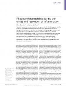
Figure 4. (a) Abundance and (b) biomass values and (c) ratio abundance on biomass for the different stations visited during KEOPS2 over sampling dates. Abundance and biomass values from Figs. 2 and 3.

The sampled stations in the Subantarctic Mode Water presented very low chlorophyll a concentration in TNS2 (0.65 mg m−3 in the upper 60 m), but much higher 10 days later, in TEW-7 and TEW-8 (average above 3 mg m−3 in the upper 60 m, with peak concentrations up to 5.0 mg m−3 ; Lasbleisz et al., 2014, their Fig. 4).


Temporal and spatial variations of zooplankton abundance and biomass

Zooplankton abundances and biomass from ZOOSCAN processed samples of the 330 µm mesh net varied from 14 × 103 to 200 × 103 ind m−2 (Fig. 2) and from 0.25 to 4.94 g C m−2 (Fig. 3), respectively. Comparisons of abundance (ind m−2 ) and biomass (g C m−2 ) between ZOOSCAN-derived data and direct measurements showed that ZOOSCAN-derived data slightly overestimated direct measurements from regression forced through the origin: slope equal to 1.0015 for abundance (R2 = 0.75, n = 37, p < 0.01) and slope equal to 1.1246 for dry weight (R 2 = 0.803, n = 19, p < 0.01). Abundance values followed a normal distribution pattern with an average of 73103 ind m−2 (SD: 42). ANOVA with main effects (stations and dates) without interaction showed clear effects for dates (p < 0.05) but not for stations. All abundance values plotted against dates (Fig. 4a) showed a general increase, and the linear regression (R 2 = 0.42, n = 37) predicted a ratio of 3.7 between abundance at the beginning and at the end of the survey. Highest abundance (above the regression line on Fig. 4a) was observed for oceanic stations within the PF meander, both for the stations of the two transects (stations TNS4, 5, 7, 8, and TEW 4, 6, 7, 8, and stations E, except for E4-West). By contrast, the lowest abundance was found to the east and north of this PF meander, as well as for the first visit to A3. One exception was station TEW5, which presented the lowest abundance, whereas nearby spatial and temporal sampling stations presented much higher abundance. Between the two visits to staBiogeosciences, 12, 4543–4563, 2015


3.3

Metazooplankton community composition and distribution

From the 330 µm mesh size net, 65 taxa were identified for the 37 stations of this study (Table 1) with 26 genera/species of copepods. Copepods contributed the bulk of the zooplankBiogeosciences, 12, 4543–4563, 2015

6

TNS TEW E A3 R FF-L

5 4

6

A

4

3

2

1

1

0

0.5

1

mg Chla

1.5

m-3

2

2.5

B

3

2

0

TNS TEW E A3 R F-L

5

gC m-2

tion A3 at the beginning and the end of the survey, the total abundance had multiplied by 3.5. The fraction 500–1000 µm (see Fig. 3) presented the most abundant number of organisms (62.0 % on average), followed by the < 500 µm fraction (18.8 % on average), the 1000–2000 µm fraction (14.2 % on average) and the > 2000 µm fraction (5.0 % on average). The contribution of the smaller size fraction (< 500 µm) increased with time from the beginning to the end of the survey (8.1 % on average), whereas the 500–1000, 1000–2000, and > 2000 µm decreased to 5.0, 0.8 and 2.3 %, respectively. However, these temporal changes were not significant in any of the four regressions due to the variability in size distribution between the stations. In addition, no clear diurnal pattern was observed from the day/night samplings performed at nine sampling dates. Log-transformed biomass values followed a normal distribution pattern. As for the abundance, ANOVA with main effects (stations and dates) without interaction for biomass values showed an effect for dates (p < 0.05) but not for stations. Average biomass was 2.32 g C m−2 (SD: 1.33), and the linear regression against time (not significant) predicted a ratio of 1.7 between biomass values at the beginning and the end of the survey (Fig. 4b). However, the biomass ratio between the two visits at station A3 showed an increase of 2.9, whereas the biomass values at station E (the Lagrangian survey) showed a slightly decreasing trend (with the exception of E4-En). The fraction > 2000 µm represented the highest biomass of organisms (57.1 % on average), followed by the 1000–2000, 500–1000 and < 500 µm fractions with 22.8, 18.2 and 1.9 % on average, respectively (see Fig. 2). None of the regressions between the percentage value and dates presented a significant correlation, and the slopes of the regression were all near to zero for the intermediate size fractions. From the beginning to the end of the survey, the largest size fraction (> 2000 µm) decreased in its contribution to the biomass (−1.5 %), whereas the contribution to the biomass increased with time by 0.1, 0.5 and 0.9 %, respectively, for the 1000–2000, 500–1000 and < 500 µm fractions. The total zooplankton biomass values presented a significant correlation (p < 0.01) with the average chlorophyll concentrations in the 100 upper metres, as well as with the integrated chlorophyll concentrations in the mixed layer depth (Fig. 5). Only stations TEW1 and TEW2 presented low zooplankton biomass for relatively high fluorescence concentrations (> 1 µg Chl a L−1 , Fig. 5a), but not versus the integrated Chl a biomass in their shallow (< 80 m) mixed layers (Fig. 5b).

gC m-2

4550

0

0

100

200

300

400

mg Chla m-2

Figure 5. Zooplankton biomass values against average Chl a in the upper 100 m (a) and against the integrated Chl a in the mixed layer depth (b) for the different stations visited during KEOPS2. Biomass values from Fig. 3.

ton community abundance with 78.4 % (SD = 13.13 %) of the counted organisms over the whole area, and copepodites represented a little more than half of the counted copepods (mean = 52.5 %, SD = 8.2 %). ANOVA with main effects (stations and dates) without interaction showed no effect either for dates or for stations, either for the percentage of copepods against the whole zooplankton abundance, or for the percentage of copepodites stages against the total copepods abundance. Nauplii represented an average 2 % of the total abundance, and showed an increasing abundance with time up to 4 %, although they were undersampled with our net. The copepod communities were dominated by Ctenocalanus citer, followed by Oithona similis and O. frigida, Metridia lucens, Scolecithricella minor, Calanus simillimus, Paraeuchaeta spp., Rhincalanus gigas, and near the coastal area Drepanopus pectinatus. Other dominant taxa were the different larval stages of euphausiids (eggs, nauplii, metanauplii, proto et metaozoe), appendicularians (Oïkopleura spp., Fritillaria spp.), chaetognaths, pteropods (Limacina retroversa) and amphipods (Themisto gaudicaudii, Hyperia spp.). Radiolarians and foraminifera were regularly sampled as well. In some stations, other taxa occurred in low numbers, such as salps. With the 120 µm mesh size net, the number of identified taxa for the 37 stations was reduced to 28 taxa (Table 1), strongly dominated by copepod species. Copepod larval forms as nauplii, undetermined copepod nauplii and copepodites, and copepodid stages of Oithona sp., Oncoea sp., and Ctenocalanus citer represented 20.4 % of organisms in 120 µm mesh size nets. Adult forms (73 % of the organisms in nets) were mainly from small and medium size copepods such as Oithona similis and O. frigida, Microsetella rosea, Oncaea spp., Triconia sp., Microcalanus pygmaeus and Scolecithricella minor. Other dominant taxa in this net were the different larval stages of euphausiids, appendicularians, chaetognaths, pteropods (Limacina antarctica), as well as, at a few stations, echinoderm larvae. Comparison between the community compositions in the two nets clearly showed that some key groups were undersampled in the 330 µm mesh net: mainly the larval stages of many copepods, small copepods such as Oithona sp. Miwww.biogeosciences.net/12/4543/2015/


4551

Table 1. List of zooplanktonic taxa collected and identified during the 2011 KEOPS2 cruise (average values for the 37 stations, in ind m−3 ). Samples from the 330 µm (left) and 120 µm mesh size (right) nets. 330 µm mesh size net

Copepods Oithona similis Oithona frigida Microsetella rosea Oncaea spp. Triconia sp. Clausocalanus laticeps Ctenocalanus citer Microcalanus pygmaeus Metridia lucens Calanus propinquus Calanus simillimus Calanoides acutus Scolecithricella minor Scaphocalanus spp. Drepanopus pectinatus Pleuromamma robusta Candacia maxima Heterorhabdus spp. Aetideus armatus Haloptilus oxycephalus Paraeuchaeta spp. Rhincalanus gigas Subeucalanus longiceps Euchirella rostramagna Gaetanus pungens Undeuchaeta incisa Undetermined nauplii Undetermined copepodites

Adult forms

Copepodites stages

8.1 14.8 1.9 1.3 8.7 3.9 35.8 0.7 9.6 0.02 6.45 1.1 9.2 0.7 0.6 0.9 rare rare rare rare 0.54 2.93 0.14 rare rare rare

2.8 2.8

120 µm mesh size net Nauplii stages

0.1 0.8 56.5 8.9 1.9 1.6 6.4 2.5 2.7 0.2 rare rare rare rare 14.29 7.34 0.02 0.04

3.1

Adult forms

Copepodites stages

489.8 71.5 79.0 58.2 20.7 1.5 47.8 23.2 4.6

1362.5 1362.5

1.4 0.2 10.1

1.62 0.41 8.4

1.4 0.4

13.7

1.1 0.4

Amphipods Themisto gaudicaudii Hyperia spp. Primno macropa Vibilia sp. Scina sp. Molluscs Limacina retroversa Limacina helicina Spongiobranchaea sp. Clio sp. Polychaetes Pelagobia sp. Tomopteris spp. Travisiopsis sp. Undetermined Appendicularians

53.6 11.4 0.1 195.7 39.3

14.1 7.9

26.63

0.04

2.1

1071.7

22.4

253.5

330 µm mesh size net

Euphausiids Undetermined species Ostracods Isopods Mysid Decapod

Nauplii stages


Adult forms

Larval forms

Eggs

0.27 2.3 0.05

6.22

32.23

Adult forms

Larval forms

Eggs

6.8

33.2

7.9 rare rare

0.26 0.86 0.10 rare rare

0.04

3.45 rare rare rare 0.22 rare rare rare 8.45


33.2

0.32

rare 149.1

9.28


4552


Table 1. Continued. 330 µm mesh size net Adult forms Thaliacea Salpa thompsoni Pyrosomid Ctenophores Cnidarians Undetermined larvae Undetermined adult Bougainvillia sp. Dimophyes arctica Pyrostephos vanhoeffeni Rosacea plicata Muggiaea bargmannae Solmundella bitentaculata Pegantha sp. Chaetognaths Radiolarians Foraminifera Meroplankton Cirripedia Echinodermata Fish Mysid Polychaeta Bivalvia

Larval forms

Eggs

Adult forms

Larval forms

Eggs

0.07 rare rare rare

rare

rare rare rare rare rare rare rare rare 4.15 0.93 0.98

crosetella rosea, Oncaea spp. Triconia sp., Microcalanus pygmaeus, Ctenocalanus citer. The impact of 120 µm mesh size and clogging on the larger planktonic organisms was difficult to assess as many groups were in any case in low density in the 330 µm mesh size net, except for the copepods Clausocalanus laticeps, Calanus simillimus and Calanoides acutus. The taxonomic distributions are presented in more detail for stations A3 (the two visits A3-1 and A3-2) and for stations E3 and E5 in Fig. 6 for the four size fractions from the 330 µm mesh size net sample, and only in the small and medium size fractions from the 120 µm mesh size net sample. The distribution pattern from the 330 µm mesh size net samples is first presented below. The zooplankton community structure in A3-1 was numerically dominated by the medium size fraction (nearly comparable to the fraction 500–1000 µm in total abundance in Fig. 2) comprising more than 50 % of copepods, characterized by the abundant cyclopoïd Oithona similis, along with unspecified calanoid copepodites, and the harpacticoid Microsetella rosea. The rest of this fraction included metanauplii of euphausiids, appendicularians, ostracods and small chaetognaths. The fraction of “large size” mesozooplankton, similar to the 1000– 2000 µm fraction counted with ZOOSCAN and representing 10.7 % of the total abundance, was composed of 98 % cope-



5.7

rare rare 0.05 rare rare

11.4 rare

pods with some major taxa (Ctenocalanus citer, Metridia lucens, Scolecithricella minor, Calanus simillimus, Scaphocalanus spp., Clausocalanus laticeps), and early copepodites of Paraeuchaeta and of Calanidae. The highest size fraction was dominated by more than 75 % by Rhincalanus gigas and amphipods Hyperia spp. and Themisto gaudicaudii. It corresponds to the fraction > 2000 µm from the ZOOSCAN which contributes to two-thirds of the mesozooplancton biomass at station A3-1 (see Fig. 2). The lowest size fraction was mainly composed of euphausiid eggs and nauplii, copepod nauplii, small forms of the pteropod Limacina retroversa and in small densities foraminifera and radiolarians. As a whole, the mesozooplancton community in A3-1 was mainly composed of herbivorous species in all fractions, such as the copepods R. gigas, C citer, O. similis, M. rosea, but also pteropod L. retroversa, appendicularians and different nauplii stages of copepods and euphausiids. In lowest densities, omnivores and detritivores (such as the copepods M. lucens, S. minor, C. simillimus) and carnivores (such as chaetognaths and amphipods, and the copepod Paraeuchaeta) were found. During the second visit to station A3 (A3-2), the size distribution in abundance was dominated by fractions with ECD < 1000 µm (up to 83 % of the total abundance, see in Fig. 3). The taxa distribution in A3-2 differed from the first visit (station A3-1) both in the “small” size fractions by an increase in



4553

Figure 6. Distributions of main taxa abundance at stations A3-1, A3-2, E3 and E5 from binocular observation. Distributions are presented from left to right for the four stations, and from top to bottom for the four size fractions (four upper bands: small, medium, large, and very large) observed in the 330 µm mesh size net samples, and for the two lower size fractions (two lower upper bands: small and medium) for the 120 µm mesh size net samples. Distributions are average values between day and night samples. For each size fraction (the four pie charts on the same horizontal band), the colour labels for the different taxa are similar.

copepod nauplii and euphausiid eggs, and in the “medium” size fraction by a large proportion of appendicularians and early copepodid stages of copepods. The two largest fractions (“large” and “very large”) were not very different at A3-1 and A3-2 in taxonomic composition and distribution (the only difference being the appearance of late larval stages of euphausiid in the “very large” fraction). The major features in taxonomic changes between stations E3 (04 November) and E5 (18 November) (Fig. 6) were the increasing contribution of calanoid copepodids in the medium and large size fractions, with the concomitant increase of contribution of these fractions to the total abundance (see also Fig. 2), and the increase of euphausiid larvae in the largest fraction. The smaller fraction presented a rather stable distribution of dominant taxa, with copepod nauplii www.biogeosciences.net/12/4543/2015/

and Limacina as dominant groups (Fig. 6). As a whole, while omnivores, carnivores and scavengers are present, the herbivorous component is strongly dominant with all these larval forms. It is of interest to note that the dominant species for the different fractions at E5 were quite similar to those at A31, but with the noticeable difference that many larval stages occurred in all size fractions, inducing the highest observed abundance during the survey (see Fig. 2), although finally representing a lower biomass (see Fig. 3). In the 120 µm mesh size net samples, the taxonomic observation generally delivered the same dominant taxa in the medium size fraction as for the 330 µm mesh size net, but with larger proportions of small copepodid forms and small adult copepods, such as Oncoea spp. and Microsetella rosea.


4554


Table 2. Isotopic composition of size-fractionated zooplankton (mean and standard deviation). Mean δ 13 C, values of acidified samples; mean δ 13 C-norm, lipid-normalized values (except for the lowest size fraction); mean δ 15 N, values of untreated samples. Fraction

Mean δ 13 C

SD δ 13 C

Mean δ 13 C-norm.

SD δ 13 C-norm.

Mean δ 15 N

SD δ 15 N

C/N

µm

‰ PDB

‰ PDB

‰ PDB

‰ PDB

‰ air

‰ air

mass

A3-1 day 20/10/2011

80 200 500 1000 2000

−25.52 −26.48 −26.20 −24.52 −25.16

0.10 0.05 0.05 0.14 0.03

−25.52 −24.00 −23.10 −22.67 −22.97

0.06 0.08 0.07 0.12 0.03

4.01 4.89 4.87 3.21 3.58

0.05 0.12 0.02 0.07 0.05

5.31 5.85 6.48 5.22 5.57

TNS-7 day 22/10/2011

80 200 500 1000 2000

−23.26 −25.18 −25.74 −24.76 −25.84

0.06 0.03 0.06 0.01 0.03

−23.26 −23.70 −23.29 −23.03 −23.21

0.07 0.02 2.00 0.00 0.06

3.45 3.41 4.29 4.21 4.60

0.09 0.15 0.04 0.06 0.22

4.55 4.85 5.82 5.10 6.01

R-2 day 26/10/2011

80 200 500 1000 2000

−27.93 −27.69 −27.11 −26.43 −26.15

0.02 0.07 0.06 0.10 0.06

−27.93 −25.84 −24.93 −24.52 −24.59

0.03 0.10 0.15 0.11 0.03

4.36 4.97 4.79 3.24 5.09

0.08 0.03 0.19 0.06 0.10

4.87 5.23 5.55 5.28 4.93

E-1 night 30/10/2011

80 200 500 1000 2000

−23.61 −25.37 −25.73 −25.26 −26.27

0.05 0.04 0.03 0.05 0.03

−23.61 −23.91 −23.26 −22.80 −22.75

0.06 0.03 0.03 0.05 0.08

3.62 3.04 3.67 3.58 4.69

0.23 0.05 0.03 0.01 0.32

4.70 4.83 5.85 5.84 6.91

E-2 day 01/11/2011

80 200 500 1000 2000

−24.62 −25.86 −25.70 −25.54 −26.12

0.04 0.02 0.04 0.02 0.02

−24.62 −23.48 −22.77 −22.45 −22.74

0.12 0.09 0.08 0.01 0.14

3.93 3.83 4.38 3.65 5.48

0.19 0.03 0.08 0.11 0.15

4.89 5.75 6.32 6.47 6.77

TEW-4 day 01/11/2011

80 200 500 1000 2000

−25.15 −25.98 −25.23 −26.01 −27.02

0.01 0.01 0.02 0.03 0.06

−25.15 −24.73 −23.39 −21.98 −21.52

0.05 0.02 0.02 0.04 0.04

4.06 3.61 3.24 3.50 5.23

0.11 0.23 0.06 0.07 0.03

4.67 4.62 5.21 7.42 8.90

TEW-8 day 02/11/2011

80 200 500 1000 2000

−22.58 −23.29 −23.73 −23.60 −23.29

0.05 0.03 0.04 0.07 0.05

−22.58 −21.00 −21.62 −21.73 −21.61

0.04 0.04 0.07 0.08 0.05

3.88 3.90 4.28 4.30 3.78

0.03 0.03 0.08 0.04 0.02

5.24 5.67 5.48 5.24 5.05

E-3 night 03/11/2011

80 200 500 1000 2000

−24.70 −25.79 −25.60 −25.67 −25.62

0.02 0.02 0.02 0.03 0.04

−24.70 −23.52 −23.24 −22.63 −23.20

0.03 0.03 0.03 0.11 0.03

3.02 3.50 4.14 3.67 4.58

0.13 0.04 0.07 0.02 0.35

4.84 5.65 5.74 6.42 5.79

E-3 day 04/11/2011

80 200 500 1000 2000

−24.82 −25.99 −26.26 −25.57 −26.71

0.04 0.02 0.02 0.03 0.03

−24.82 −23.51 −22.79 −22.41 −22.19

0.07 0.05 0.05 0.03 0.06

2.98 3.58 3.90 3.68 5.23

0.10 0.06 0.04 0.06 0.48

4.71 5.85 6.86 6.54 7.92

F-L day 06/11/2011

80 200 500 1000 2000

−23.69 −24.06 −24.59 −24.31 −24.64

0.03 0.01 0.03 0.03 0.01

−23.69 −21.42 −21.62 −21.58 −21.48

0.05 0.06 0.14 0.07 0.04

3.66 4.20 5.08 4.44 5.00

0.09 0.10 0.08 0.10 0.17

5.87 6.02 6.35 6.11 6.55

Station Date




4555

Table 2. Continued. Fraction

Mean δ 13 C

SD δ 13 C

Mean δ 13 C-norm.

SD δ 13 C-norm.

Mean δ 15 N

SD δ 15 N

C/N

F-L night 06/11/2011

80 200 500 1000 2000

−21.77 −23.41 −24.67 −23.75 −22.38

0.02 0.03 0.08 0.05 0.01

−21.77 −20.96 −21.01 −21.58 −21.53

0.01 0.03 0.12 0.06 0.02

4.06 3.54 4.41 4.06 3.61

0.10 0.03 0.09 0.05 0.06

4.80 5.83 7.05 5.54 4.21

E-4W day 11/11/2011

80 200 500 1000 2000

−23.26 −24.66 −25.05 −24.21 −25.01

0.08 0.05 0.02 0.02 0.02

−23.26 −22.93 −22.70 −22.31 −21.38

0.02 0.05 0.02 0.08 0.01

3.17 3.43 3.85 3.97 4.64

0.12 0.11 0.07 0.08 0.17

5.14 5.10 5.73 5.28 7.53

E-4W night 11/11/2011

80 200 500 1000 2000

−23.24 −24.83 −25.30 −24.83 −24.92

0.03 0.07 0.06 0.07 0.06

−23.24 −23.10 −22.81 −22.52 −22.10

0.05 0.13 0.06 0.04 0.07

2.97 3.33 3.94 3.91 3.85

0.29 0.06 0.02 0.04 0.12

4.72 5.09 5.86 5.68 6.20

E-4E night 12/11/2011

80 200 500 1000 2000

−23.47 −25.24 −26.07 −26.02 −27.12

0.04 0.04 0.04 0.07 0.11

−23.47 −22.59 −19.61 −18.92 −17.64

0.04 0.10 0.06 0.45 0.26

2.42 3.77 4.72 4.82 4.76

0.14 0.06 0.14 0.20 0.59

5.14 6.03 9.88 10.53 12.93

E-4E day 13/11/2011

80 200 500 1000 2000

−23.65 −25.32 −25.97 −25.38 −25.76

0.02 0.06 0.02 0.08 0.11

−23.65 −21.90 −20.81 −21.06 −22.67

0.03 0.11 0.17 0.21 0.09

3.17 4.02 4.40 4.63 3.96

0.52 0.15 0.08 0.08 0.49

5.53 6.81 8.56 7.72 6.48

A3-2 day 16/11/2011

80 200 500 1000 2000

−22.82 −23.58 −24.19 −23.44 −23.09

0.09 0.02 0.04 0.05 0.04

−22.82 −22.42 −22.38 −21.91 −21.42

0.22 0.05 0.15 0.04 0.07

1.71 3.89 5.45 4.66 3.71

0.17 0.02 0.16 0.07 0.20

4.49 4.53 5.19 4.89 5.04

A3-2 night 16/11/2011

80 200 500 1000 2000

−22.42 −23.47 −23.98 −24.99 −23.22

0.02 0.04 0.05 0.04 0.05

−22.42 −22.31 −22.33 −20.38 −21.46

0.06 0.09 0.16 0.10 0.04

2.43 3.98 4.90 5.04 4.11

0.09 0.16 0.06 0.04 0.06

4.44 4.53 5.02 8.01 5.13

E-5 day 18/11/2011

80 200 500 1000 2000

−25.88 −26.64 −26.01 −25.89 −27.74

0.06 0.36 0.03 0.05 0.01

−25.88 −23.91 −23.04 −23.00 −21.59

0.09 0.30 0.04 0.09 0.20

2.45 3.10 3.24 3.30 6.19

0.01 0.22 0.17 0.02 0.14

3.71 6.11 6.35 6.27 9.56

E-5 night 19/11/2011

80 200 500 1000 2000

−26.18 −25.90 −26.07 −25.90 −27.39

0.03 0.02 0.01 0.04 0.02

−26.18 −22.64 −22.54 −22.71 −22.83

0.07 0.05 0.04 0.09 0.10

2.87 3.45 3.61 3.76 4.37

0.27 0.09 0.02 0.05 0.38

6.01 6.64 6.92 6.58 7.97

Station

Copepod nauplii and early copepodid contributed with high abundance (see Table 1) to the small size fraction. To compare the taxonomic composition between all stations, a cluster dendrogram quantifying the compositional www.biogeosciences.net/12/4543/2015/

similarity of taxa distributions between the different stations was constructed from the Bray–Curtis coefficient using the 330 µm mesh size net samples which presented the largest number of taxa. Figure 7 presents the cluster dendrogram and Biogeosciences, 12, 4543–4563, 2015

4556


Table 3. Mean (±SD) stable isotope values of the main groups of organisms sorted in the largest size fraction (> 2000 µm). n is the number of samples analysed. Groups Salps Copepods Euphausiacea Amphipods Pteropods Gymnosoms Chaetognaths Polychaetes Tomopteris Fish larvae

n

δ 13 C (‰ )

δ 15 N (‰ )

12 15 12 9 5 12 3 3

−22.36 ± 0.82 −21.98 ± 0.95 −21.03 ± 2.34 −23.19 ± 0.24 −23.44 ± 0.04 −22.94 ± 0.18 −22.52 ± 0.03 −21.60 ± 0.05

3.87 ± 1.29 4.40 ± 0.54 4.24 ± 0.63 4.14 ± 0.41 4.56 ± 0.09 5.93 ± 0.60 7.72 ± 0.06 5.99 ± 0.08

the PF meander and including eastern stations east of PF (F-L and TW7), and a second group of dispersed stations (BC group 2, with less than 80 % similarity – differences in day–night sampling were not considered in this analysis), including the R2 station on the western side of the Kerguelen Plateau characterized by higher abundance of large calanoid copepods such as Rhincalanus gigas and Paraeuchaeta spp., the TEW1 and TEW2 stations, near the Kerguelen coast and dominated by Drepanopus pectinatus and bivalvia meroplanktonic larvae, the TNS1and TNS2 stations in Subantarctic Surface Water waters dominated by medium size cyclopoid and calanoids and larval forms of euphausiids, the A3 and TNS10 stations in the southern part (see detail below), and stations TEW3, TEW5, TEW8, which were characterized by relative differences in very few taxa, compared to other stations of the TEW transect (high density of Metridida lucens in TEW3, relatively lower density of Ctenocalanus citer in TEW5, and high density of Triconia sp. in TEW8). 3.4

Figure 7. Dendrogram (a) and MDS plot (b) produced by the clustering of the 37 samples (28 stations, among them nine stations with day–night sampling) during KEOPS2 based on the density (ind m−3 ) of mesozooplankton taxa. Density values were fourthroot-transformed prior to analysis of the Bray–Curtis similarity matrix. The stress statistic for the MDS plot is 0.12.

its associated 2-D multidimensional scaling plot. This analysis showed a high degree of similarity across the whole region related to the initial phase of zooplankton development. The shelf stations presented the highest level of dissimilarity compared to the other stations. The cluster dendrogram sliced at 80 % similarity distinguished two BC groups: a first one (BC group 1, with more than 80 % similarity) grouping the oceanic stations within Biogeosciences, 12, 4543–4563, 2015

Isotopic composition of size-fractionated zooplankton and within zooplankton taxa

A wide range of δ 13 C (> 8 ‰ ) and δ 15 N (> 4 ‰) values were recorded among zooplankton size fractions and stations (Table 2). A slight general increase of δ 13 C with increasing size fraction was observed, while the difference was not significant due to wide differences between sites (F = 1.818, p = 0.132) (Fig. 8a). A significant increase in δ 15 N with increasing size was observed (F = 11.67, p < 0.001), particularly between the two smallest fractions (80–200 and 200– 500 µm) and the three largest ones (Fig. 8b). However, no significant difference in mean δ 15 N was apparent between the 500–1000 and > 2000 µm fractions, while the 1000–2000 µm fraction exhibited a slightly lower δ 15 N than the two others. Within each size fraction, no difference was observed between mean day and night δ 13 C and δ 15 N values (p > 0.05 for both), in spite of differences at site level (Table 2). Thus, for both δ 13 C and δ 15 N values, the main difference occurred between the two smallest size classes (< 500 µm) and the three largest ones (> 500 µm). At the station level, mean δ 13 C and δ 15 N values differed. Station R2 presented the lowest mean δ 13 C (−25.26 ‰) and the highest mean δ 15 N (4.49 ‰), while stations F-L, TEW-8 and E4-E were characterized by the highest δ 13 C (> −21.2 ‰) and rather high δ 15 N values (> 4 ‰ ). All the other stations exhibited mean δ 13 C values (from −23.26 to −21.76 ‰) and a wide range of mean δ 15 N values (from 3.63 to 4.25 ‰). Differences in mean δ 15 N between small (< 500 µm) and large (> 500 µm) zooplankton size fractions were low in Tgroup 1 (0.3 ‰), increased in T-group 5 (0.6 ‰) and were highest at most stations located in the eddy (Fig. 9). This trend suggested higher food overlap among size fractions in zooplankton associated with phytoplankton T-group 1 and Tgroup 5, and more partitioned food resources in phytoplankwww.biogeosciences.net/12/4543/2015/


4557

Table 4. Seasonal variations of zooplankton abundance and biomass from KEOPS2 (15 October to 20 November 2011) and KEOPS1 (19 January to 13 February 2005) surveys with contribution of different size fractions (< 500, 500–1000; 1000–2000 and > 2000 µm). The reference stations were A3 (shelf waters) and C11 (oceanic waters) for KEOPS1 (see Carlotti et al. (2008), their Figs. 3 and 5), and A3 (shelf waters) and TNS6-TNS5 and E4E-E5 (oceanic waters) for KEOPS2. KEOPS2 Area

Date

Shelf waters

Abundance

20–22/10

13–16/11

22–28/1

4–5/2

12/2

× 106 m−2

26

90

600

700

450

< 500 µm

10 %

34 %

55 %

46 %

41 %

500–1000 µm 1000–2000 µm > 2000 µm

60 % 23 % 7%

50 % 13 % 3%

32 % 12 % 1%

35 % 18 % 2000

1.5 1,5

-28,0 -28.0

2500

Size classes (µm)

Figure 8. Distribution of δ 13 C (a) and δ 15 N (b) of zooplankton across size fractions during KEOPS2. White symbols represent day; black symbols represent night.


KEOPS1

ton T-group 2 and T-group 3, as indicated by a more even increase in δ 15 N with zooplankton size at these stations. The smaller size fraction (80–200 µm) was differently composed according to stations, being dominated either by diatoms (A3-2, E-4W), foraminifera (A3-1), small copepods (R2), or a mixture of these groups (most stations). Copepods, eggs, thecosome pteropods foraminifera and small aggregates contributed to 200–500 µm fractions. The following size fractions (500–1000, 1000–2000 and > 2000 µm) were all dominated by copepods (60–95 %), but amphipods, euphausiids, appendicularians and chaetognaths increased in abundance from the 500–1000 to the 1000–2000 µm fractions. The largest size fraction (> 2000 µm) was dominated by Rhincalanus gigas and euphausiid larvae or juveniles. Large chaetognaths completed this large fraction. Thus, differences in specific composition of size fractions, particularly the smallest and the largest, could result in isotopic differences between stations within a size fraction. For example, when diatoms dominated the 80–200 µm fraction, δ 15 N values were lower than when composed of foraminifera or small copepods (2–3 and 4–4.5 ‰, respectively).


4558

F. Carlotti et al.: Mesozooplankton structure and functioning 4 4.1

Figure 9. Distribution of δ 13 C (left column, a) and δ 15 N (right column, b) values across zooplankton size fractions for four of the five T-groups of stations identified by Trull et al. (2015) for phytoplankton. Station E4-E is included here in T-group 5 instead of T-group 2. From top to bottom: a1 and b1, T-group 1 (diamonds); a2 and b2, T-group 2 (triangles); a3 and b3, T-group 3 (dots); and a4 and b4, Tgroup 5 (squares). T-group 4 included coastal stations not sampled in the zooplankton analysis.

Groups of organisms individualized in the > 2000 µm fraction presented highly different isotopic signatures according to their main feeding behaviours (Table 3). Filtering salps presented the lowest δ 15 N (< 4 ‰), the mostly herbivorous copepods, amphipods, euphausiids, and pteropods intermediate values (4 to 4.6 ‰), while predatory chaetognaths, fish larvae and polychaetes exhibited higher δ 15 N values (> 5 ‰). Thus, δ 15 N differences of the > 2000 µm fraction between stations resulted mainly from the relative contributions of these groups to bulk samples (e.g. higher proportion of salps and euphausiids at A3-2, and large chaetognaths at E5). Accordingly, differences in δ 13 C values could be linked to difference in both size and composition of the ingested food. The lower δ 13 C recorded in gymnosomes and copepods suggested the consumption of small phytoplankton particles, while the higher δ 13 C of euphausiids suggested a consumption of larger-sized phytoplankton. Higher δ 13 C in euphausiids compared to copepods was also observed in Arctic seas (Schell et al., 1998).


Discussion Zooplankton development during the 2011 early spring bloom and comparison with other seasons

In high latitudes, zooplankton first increase in abundance more than biomass in response to initial phytoplankton spring bloom due to stimulated reproduction of overwintering adults of dominant copepods. This induces a lag-time in the grazing response of herbivorous zooplankton at the beginning of blooms, which further promotes the rapid phytoplankton accumulation. Higher phytoplankton concentrations then stimulate grazing by overwintering stages and new cohorts which results in build-up of zooplankton biomass. With the succession of new cohorts in full bloom conditions (> 0.8 mg Chl a m−3 ), continuous egg production and individual growth induce proportional increase of abundance and biomass. Such a response of zooplankton to an early phase of the north-eastern Kerguelen bloom was observed during the Lagrangian survey within the stationary meander of the Polar Front (stations E1 to E5, except E4-W, Figs. 2, 3 and 4). The average integrated Chl a concentrations were rather low (0.49 to 0.77 µg Chl a m−3 ) for these E stations and but slightly higher than the previous weeks – transects TNS and TEW- (Lasbleisz et al., 2014). The POC was constant in the surface layer up to the time of E3, with an average of 83 mg C m−3 , and then slightly increased at E4 and E5 (with an average up to 109 mg C m−3 ) (Lasbleisz et al., 2014). Zooplankton densities increased from 60 × 103 ind m−2 (E1d) to 200 × 103 ind m−2 (E5-d) whereas biomass gradually decreased (excepted E4-E-n) from 2.3 g C m−2 (E1-d) to 1.7 g C m−2 (E5-n). Two processes may favour the shift towards smaller size classes. Firstly, the contribution of the larger size classes to biomass decreased with time (Fig. 3) due to the reduction of initial standing stock of overwintering zooplankton by mortality and by investment in egg production. The dominant overwintering copepods (Ctenocalanus citer, Rhincalanus gigas) are known to be strong seasonal migrants able to spawn in early spring even at low chlorophyll concentrations (Schnack-Schiel, 2001; Atkinson, 1998), i.e. before the full bloom conditions. Moreover, smaller copepod species and copepodids of large copepods may better exploit these low food concentrations (Atkinson et al., 1996), allowing individuals to develop and grow, whereas large copepods are food limited. The response to chlorophyll increase in waters above the plateau (station A3 in Fig. 4c) was proportional in abundance and biomass (threefold higher at A3-2 than at A3-1). Lasbleisz et al. (2014) mention that the Chl a increase at station A3-2 was accompanied by an increase of the Phaeo : Chl a ratio, reflecting a potential higher grazing activity. The mesozooplankton at A3-2 (see Fig. 6) presented a grazer community structure able to feed on a wide spectrum of cells from small diatoms to phytodetritus aggregates, as observed www.biogeosciences.net/12/4543/2015/

F. Carlotti et al.: Mesozooplankton structure and functioning at this station (Lasbleisz et al., 2014; Laurenceau-Cornec et al., 2015), as well as small nano-/microzooplankton (Christaki et al., 2014) and carnivorous zooplankton. Compared to A3-1, the medium size and small size mesozooplankton fractions had a much larger contribution of microphagous organisms (appendicularians, copepod nauplii, etc.) which could quickly remove the smaller planktonic forms (below 20 µm). The larger zooplankton size fractions were a mixture of efficient grazers on large diatoms (> 20 µm), omnivores and detritivores able to feed on aggregates, and carnivores consuming micro- and mesozooplanckton. The mesozooplankton biomass stocks observed at the beginning of the KEOPS2 cruise (Table 4) were around 1.7 g C m−2 above the plateau (A3) and 1.2 g C m−2 in oceanic waters (TNS transect). Oceanic biomass slightly increased during the cruise, except the biomass observed in the eastern bloom (station F-L) in the Polar Front zone (above 4 mg C m−2 ), and station A3 also presented biomass around 4 mg C m−2 at the end of the survey. These different results during KEOPS2 suggest that the zooplankton community is able to respond to the growing phytoplankton blooms earlier on the plateau than in the oceanic waters, where complex mesoscale circulation stimulates initial more or less ephemeral blooms before a broader bloom extension. Due to our constrained sampling for oceanic stations, it was not possible to determine whether the observed zooplankton biomass variability between oceanic stations was linked to enhanced local production (except for stations near the permanent Polar Front sustaining high level of production). Our results in the quasi-Lagrangian survey within the meander suggests that the heterogeneous primary production linked to oceanic mesoscale activity in the early bloom phase may stimulate the production of new zooplankton cohorts, without sustaining individual growth, slowing down the built-up of new zooplankton biomass. In addition, potential predation on mesozooplankton by euphausiid populations was expected, from observations of the increasing contribution of euphausiid larval stages in our Bongo net samples (see Fig. 6) and of long faecal pellets in gel traps (Laurenceau-Cornec et al., 2015). In contrast, stations F-L (06 November) and A3-2 (16 November) presented the highest biomass (maintained below 5 g C m−2 ) observed in November (Figs. 4 and 5) and a similar ratio of abundance to biomass, around 20 × 103 ind per g C (Fig. 4c) and a lower contribution of smaller size fractions (ESD < 1000 µm) to total biomass comparatively to station E5. These characteristics could be the results of a phytoplankton-sustained zooplankton development over the previous weeks. 4.2

Comparison with previous results

If we group our observations of KEOPS1 and KEOPS2 (Table 4), the zooplankton seems to continuously increase from mid-October to early February, with a ratio higher on shelf www.biogeosciences.net/12/4543/2015/

4559 waters (abundance ×20 and biomass ×9) than in oceanic waters (abundance ×3 and biomass ×2.5). After early February, the zooplankton community structure remained rather stable (Carlotti et al., 2008). Over the whole spring to summer seasons, the small size fractions (< 500 and 500–1000 µm) significantly contribute to the increase in abundance (from 70 to 85 %), with the production of calanoid copepod larval stages and large numbers of cyclopoid copepods, whereas the increase in biomass is mainly due to the fraction 1000– 2000 µm with calanoid copepod late larval stages (with a contribution doubling from spring to summer). The taxonomic composition did not show major differences between shelf and oceanic waters, except that the contribution of copepods to the whole mesozooplankton was higher in oceanic waters than on the shelf, and these taxonomic patterns were quite similar between the KEOPS 1 (see Fig. 7 in Carlotti et al., 2008) and KEOPS2 survey (Fig. 6). The use of different laboratory technologies (Lab OPC during KEOPS1 and ZOOSCAN during KEOPS2) to optically measure and size plankton organisms from net haul samples must be considered. In their comparative study between LOPC and ZOOSCAN, Schultes and Lopes (2009) found good agreement in the normalized biomass size spectra (NBSS) for particles in the size range of 500 to 1500 µm in equivalent spherical diameter (ESD). Several disparities for smaller and larger particles size range in their study were due both to in situ sampling (LOPC and net have different sampling efficiencies), in situ vs. lab counting (LOPC counts any particles, not only zooplankton, with potential overlapping between particles, whereas ZOOSCAN samples are carefully distributed on a scanned window), etc. Our present comparison of estimated abundance and biomass for KEOPS1 and KEOPS2 is based on similar sampling protocols with a 330 µm mesh net on the Bongo frame, and in both cases a delicate laboratory protocol. The flow-through system used with the Lab-OPC for KEOPS1 samples was controlled to avoid coincidence of organisms counted by the laser (count rate at 20 particles min−1 ; see Carlotti et al., 2008) and organisms were carefully separated on the ZOOSCAN window for the KEOPS2 samples. In both studies, a large number of individuals were counted (1000 particles per samples) to correctly count and size larger organisms. Finally, the lower and higher range of counted and measured zooplankton organisms are mainly due to the 330 µm mesh net efficiency, and the abundance and biomass results of both studies might be compared. In addition to the recent survey of the CPR data for the region (see in Introduction), which shows the strong development of mesozooplankton abundance in October–November, the overall results of KEOPS 1 and 2 in terms of seasonal changes in abundance and biomass values are highly consistent with the information provided by Semelkina (1993) and Razouls et al. (1996, 1998). During the SKALP cruises, all around the Kerguelen Islands (46–52◦ S, 64–73◦ E), Semelkina (1993, her Table 1) observed an increase from Biogeosciences, 12, 4543–4563, 2015

4560


62 × 103 ind m−2 in July–August 1987 (average values between 0 and 200 m depth for the whole sampled area, nearly double from 0–1000 m) to 570 × 103 ind m−2 in February 1988 (values between 0 and 200 m, 100 × 103 ind m−2 more in the layer 200–400 m). In terms of biomass, assuming a carbon content to be 50 % of body dry weight, the biomass increase in the upper 200 m was from 2.2 g C m−2 to 19 g C m−2 . The sampled areas during the SKALP cruises covered a much larger area than that studied during KEOPS2, but these average values corresponded to those observed on the eastern side of the Kerguelen Islands (see Semelkina (1993), her Fig. 2). Concerning the taxonomic composition of the mesozooplankton, this author mentioned no seasonal variations but differences in population development and distribution. Razouls et al. (1998) presented the seasonal changes in copepod distributions at the KERFIX station, a fixed timeseries station, situated 60 miles south-west of the Kerguelen Islands (50◦ 400 S, 68◦ 250 E), in 1700 m of water, characteristic of the Permanently Open Ocean Zone (POOZ). The copepod abundance sampled from vertical hauls (300 m – surface) ranged from less than 30 × 103 ind m−2 in winter and 45 × 103 ind m−2 in October up to 222 × 103 ind m−2 in January. The nearest station during KEOPS1 and 2 was station R2 which presented biomasses (respectively abundance densities) of 10.7 g C m−2 (272 × 103 ind m−2 ) in February 2005 and 4.5 g C m−2 (80 × 103 ind m−2 ) in November 2011. Abundances during KEOPS1 and 2 were largely dominated (> 80 %) by copepods (Carlotti et al., 2008, their Fig. 7; distribution not shown for KEOPS2). In addition, during a coastal annual survey in Morbihan Bay at the Kerguelen Islands, Razouls et al. (1996) found a ratio of 10 between winter and spring–summer mesozooplankton density (from 2 to 20 × 103 ind m−3 ) and a ratio of 20 for the corresponding biomass (from 20 to 400 mg DW m−3 ). 4.3

Effects of primary production on trophic pathways through mesozooplankton

The KEOPS2 cruise illustrates the complexity of the phytoplankton bloom in spring in the oceanic waters of the Kerguelen Islands, linked to the intense mesoscale activity both in species diversity and spatial production. Comparatively, the mesozooplankton presents initial standing biomass stocks between 1 and 2 g C m−2 everywhere in the region, ready to exploit any new phytoplankton production. When this occurs, the initial response is to produce new cohorts which grow further as the bloom builds up, delaying the major grazing impact when these cohorts reach the later stages. Sustained full blooms at plateau stations or permanent fronts favour the highest and longest secondary production rate. The spring period usually shows the greatest increase in grazing pressure on phytoplankton (Razouls et al., 1998). The comparison of the sinking particle composition at early and advanced stages of the bloom at station A3 Biogeosciences, 12, 4543–4563, 2015

(Laurenceau-Cornec et al., 2015 for KEOPS2; Ebersbasch et al., 2008 for KEOPS1) shows that early bloom stage is characterized by particles dominated by phyto-aggregates due to relatively weak grazing pressure on phytoplankton stocks, whereas faecal aggregates characterized the vertical matter flux as soon as zooplankton grazing substantially affects the phytoplankton stock. The qualitative composition of the bloom had a direct impact in terms of species dominance (mostly herbivorous species) and biochemical composition of the zooplankton organisms. The spatial differences observed in isotopic signatures of phytoplankton were tracked up to the higher zooplankton levels and showed the impact of the food source. Differences in the isotopic ratios of zooplankton were observed between stations during the KEOPS2 survey. Station R2 exhibited a 2.2 ‰ lower δ 13 C than stations located on the plateau (A3) or in the eddy (E1 to E5), while δ 13 C of stations located in the open ocean (F-L) was increased by ∼ 1.5 ‰ compared to them. A similar increase in carbon isotopic signature was observed by Trull et al. (2015) for phytoplankton, with the lowest δ 13 C at the HNLC reference station (R2) and the highest at stations located in the open ocean downstream near the Polar Front (F-L, TEW8) (Fig. 10). The trophic relationship between mesozooplankton and phytoplankton (Trull et al., 2015) was evidenced by the significant positive correlation of their δ 13 C values (δ 13 CZooplankton = 0.745 δ 13 CPhytoplankton − 5.465, r = 0.85, p < 0.001). As shown in Fig. 10, mean δ 13 C values of zooplankton were related to those of phytoplankton, testifying to the consumption of phytoplankton by zooplankton at station level. The mean trophic fractionation factor from phytoplankton to zooplankton was 0.40 ± 0.71 ‰ for δ 13 C and 2.69 ± 0.65 ‰ for δ 15 N. These values corresponded to a mean increase lower than one trophic level, if we apply the commonly used trophic fractionation factors (1 ‰ for δ 13 C and 3.14 ‰ for δ 15 N) that are in agreement with previous studies on zooplankton (Fry and Quinones, 1994). Such low values again indicated a dominance of herbivory among zooplankton organisms, which confirmed the conclusions based on zooplankton composition. The mean increase in δ 15 N in small zooplankton size classes (from 80–200 to 500–1000 µm) was higher than among larger size fractions (from 500–1000 µm to > 2000 µm) (1 ‰ and 0.28 ‰ respectively). This lower increase in mean δ 15 N from 500–1000 to > 2000 µm suggested a high food overlap among the three largest size fractions, with a dominance of herbivorous organisms. Within the largest size fraction (> 2000 µm), an increase in trophic level (δ 15 N) was observed from filtering (salps) and mostly herbivorous organisms (copepods, pteropods, etc.) to predatory carnivores (chaetognaths), as observed in other regions (Tarling et al., 2012; Banaru et al., 2014). While different feeding behaviours can be observed among euphausiids (Mauchline, 1980), most euphausiids collected during the KEOPS2 survey were mainly herbivores or omnivores www.biogeosciences.net/12/4543/2015/


4561 5

Figure 10. Mean δ 13 C and δ 15 N values of phytoplankton (5– 210 µm) (Trull et al., 2015) and zooplankton (200 to > 2000 µm) (present study) for stations sampled during the KEOPS2 cruise. Symbols correspond to the phytoplankton groups based on chemometric measurements identified by Trull et al. (2015): diamonds, T-group 1; triangles, T-group 2; dots, T-group 3; squares, T-group 5.

with a δ 15 N varying between 3.5 and 5.0 ‰ for individuals > 2000 µm, a range value already observed in the Southern Ocean (Gurney et al., 2001; Schmidt et al., 2003). High feeding overlap across size-fractionated zooplankton is reported in most studies (Fry and Quiñones, 1994; Bode et al., 2007) and may increase during food shortage (Tarling et al., 2012; Banaru et al., 2014). During KEOPS2, the highest food overlap among zooplankton size fractions seemed to be associated with phytoplankton T-group 1 and T-group 5 in which small-sized cells dominated, while more partitioned food resources among size fractions seemed to occur in zooplankton associated with phytoplankton T-group 2 and T-group 3, where large phytoplankton cells dominated (Trull et al., 2015).The direct comparison between stable isotope values of size-fractionated zooplankton and their abundance or biomass in water masses is difficult. Zooplankton isotopic values are firstly related to those of the phytoplankton they feed on, themselves being linked to water characteristics and nutrient cycling (Trull et al., 2015). The stable isotope values recorded during the KEOPS2 survey suggest a general increase in herbivory in zooplankton during the bloom in accordance with the increase in the abundance of smallsized zooplankton, and corroborate the finding of Lasbleiz et al. (2015) based on the Phaeo : Chl a ratio.

Conclusions

The complexity of the oceanic processes inducing the largescale phytoplankton bloom in the eastern area of the Kerguelen Islands occurs over scales ranging from the very large (1000 s of kilometres) down to the submesoscales (10 s of kilometres), marked by intense oceanic–plateau interactions linked to the meandering circulation of the Polar Front (PF) and by a myriad of secondary circulations linked to circulations resulting in a patchy distribution of the new production with different intensity and duration. The KEOPS2 survey addressed the challenge of examining the large-scale phytoplankton bloom that forms over and downstream of the Kerguelen Plateau in the most productive season, but also of carrying out observations at a finer resolution in order to understand the influence of spatial and temporal variability of biogeochemical and biological processes on the overall regional ecosystem dynamics and carbon export. Our results on the mesozooplankton dynamics during KEOPS2 suggest that the zooplankton community maintains relatively high winter stocks both on the plateau and in the oceanic waters, mostly distributed in mesopelagic waters, ready to exploit the early phytoplankton blooms. The timing and intensity of the bloom on the plateau allow an earlier and longer period favourable for zooplankton development and growth compared to the surrounding oceanic waters. A longer lag-time (several weeks) between an initial reproduction phase of the zooplankton organisms and the biomass increase, and thus their grazing impact, was clearly observed in oceanic waters. Acknowledgements. We thank the project coordinator, S. Blain, and the chief scientist on board, B. Quéguiner, for inviting us to take part in the KEOPS2 project and for supplying data. We thank the captain Bernard Lassiette and crew of the R/V Marion Dufresne for their support aboard. We also thank G. Guillou LIENSs Laboratory at the Université de La Rochelle for processing stable isotope analysis, and Tom Trulls and Marc Pagano for valuable comments on the manuscript. We thank the three reviewers for their comments and suggestions, which significantly contributed to improving the quality of the publication, and M. Paul for English proof-reading. This work was supported by the French Research program of INSU-CNRS LEFE – CYBER (“Les enveloppes fluides et l’environnement – Cycles biogéochimiques, environnement et ressources”), the French ANR (Agence Nationale de la Recherche, ANR-10-BLAN-0614 of SIMI-6 program, and ANR-09-CEXC-006-01 to M. Zhou and F. Carlotti), LABEX OT-MED (no. ANR-11-LABX-0061), the French CNES (Centre National d’Etudes Spatiales) and the French Polar Institute IPEV (Institut Polaire Paul-Emile Victor). Edited by: T. Trull



4562 References Atkinson, A.: Life cycle strategies of epipelagic copepods in the Southern Ocean, J. Marine Syst., 15, 1–4, 289–311, 1998. Atkinson, A., Shreeve, R. S., Pakhomov, E. A., Priddle, J., Blight, S. P., and Ward, P.: Zooplankton response to a phytoplankton bloom near South Georgia, Antarctica, Mar. Ecol.-Prog. Ser., 144, 195– 210, 1996. Banaru, D., Carlotti, F., Barani, A., Gregory, G., Neffati, N., and Harmelin-Vivien, M.: Seasonal variation of stable isotope ratios of size-fractionated zooplankton in the Bay of Marseille (NW Mediterranean Sea), J. Plankton Res., 36, 145–156, 2014. Blain, S., Quéguiner, B., Armand, L., Belviso, S., Bombled, B., Bopp, L., Bowie, A., Brunet, C., Brussaard, C., Carlotti, F., Christaki, U., Corbiere, A., Durand, I., Ebersbach, F., Fuda, J. L., Garcia, N., Gerringa, L., Griffiths, B., Guigue, C., Guillerm, C., Jacquet, S., Jeandel, C., Laan, P., Lefèvre, D., Lo Monaco, C., Malits, A., Mosseri, J., Obernosterer, I., Park, Y. H., Picheral, M., Pondaven, P., Remenyi, T., Sandroni, V., Sarthou, G., Savoye, N., Scouarnec, L., Souhaut, M., Thuiller, D., Timmermans, K., Trull, T., Uitz, J., van Beek, P., Veldhuis, M., Vincent, D., Viollier, E., Vong, L., and Wagener, T.: Effect of natural iron fertilization on carbon sequestration in the southern ocean, Nature, 446, 1070– 1074, 2007. Blain, S., Quéguiner, B., and Trull, T.: The natural iron fertilization experiment KEOPS (Kerguelen Ocean and Plateau Compared Study): an overview, Deep-Sea Res. Pt. II, 55, 559–565, 2008. Blain, S., Renaut, S., Xing, X., Claustre, H., and Guinet, C.: Instrumented elephant seals reveal the seasonality in chloropyll and light-mixing regime in the iron fertilized Southern Ocean, Geophys. Res. Lett., 40, 6368–6372, 2013. Bode, A., Alvarez-Ossorio, M. T., Cunha, M. E., Garrido, S., Peleteiro, J. B., Porteiro, C., Valdés, L., and Varela, M.: Stable nitrogen isotope studies of the pelagic food web on the Atlantic shelf of the Iberian Peninsula, Prog. Oceanogr., 74, 115–131, 2007. Bodin, N., Le Loc’h, F., and Hily, C.: Effect of lipid removal on carbon and nitrogen stable isotope ratios in crustacean tissues, J. Exp. Mar. Biol. Ecol., 341, 168–175, 2007. Bray, J. R. and Curtis, J. T.: An ordination of the upland forest communities of southern Wisconsin, Ecol. Monogr., 27, 273–279, 1957. Carlotti, F., Botha, D., Nowaczyck, A., and Lefèvre, D.: Structure, biomass, feeding and respiration of the mesozooplankton community during KEOPS, Deep-Sea Res. Pt. II, 55, 720–733, 2008. Christaki, U., Lefèvre, D., Georges, C., Colombet, J., Catala, P., Courties, C., Sime-Ngando, T., Blain, S., and Obernosterer, I.: Microbial food web dynamics during spring phytoplankton blooms in the naturally iron-fertilized Kerguelen area (Southern Ocean), Biogeosciences, 11, 6739–6753, doi:10.5194/bg-116739-2014, 2014. Clarke K. R. and Warwick R. M.: Change in Marine Communities: an Approach to Statistical Analysis and Interpretation, 2nd Edn., Primer-E Ltd, Plymouth, UK, 2001. DeNiro, M. J., and Epstein, S.: Influence of diet on the distribution of carbon isotopes in animals, Geochim. Cosmochim. Ac., 42, 495–506, 1978. d’Ovidio, F., Della Penna, A., Trull, T. W., Nencioli, F., Pujol, I., Rio, M. H., Park, Y.-H., Cotté, C., Zhou, M., and


F. Carlotti et al.: Mesozooplankton structure and functioning Blain, S.: The biogeochemical structuring role of horizontal stirring: Lagrangian perspectives on iron delivery downstream of the Kerguelen plateau, Biogeosciences Discuss., 12, 779–814, doi:10.5194/bgd-12-779-2015, 2015. Farías, L., Florez-Leiva, L., Besoain, V., Sarthou, G., and Fernández, C.: Dissolved greenhouse gases (nitrous oxide and methane) associated with the naturally iron-fertilized Kerguelen region (KEOPS 2 cruise) in the Southern Ocean, Biogeosciences, 12, 1925–1940, doi:10.5194/bg-12-1925-2015, 2015. Fry, F. and Quiñones, R.. B.: Biomass spectra and stable isotope indicators of trophic level in zooplankton of the northwest Atlantic, Mar. Ecol. Prog.-Ser., 112, 201–204, 1994. Gorsky, G., Ohman, M. D., Picheral, M., Gasparini, S., Stemmann, L., Romagnan, J. B., Cawood, A., Pesant, S., Garcia-Comas, C., and Prejger, F.: Digital zooplankton image analysis using the ZooScan integrated system, J. Plankton Res., 32, 285–303, 2010. Grosjean, P., Picheral, M., Warembourg, C., and Gorsky, G.: Enumeration, measurement, and identification of net zooplankton samples using the ZOOSCAN digital imaging system, ICES J. Mar. Sci., 61, 518–525, 2004. Gurney, L. J., Froneman, P. W., Pakhomov, E. A., and McQuaid, C. D.: Trophic positions of three euphausiid species from the Prince Edward Islands (Southern Ocean): implications for the pelagic food web structure, Mar. Ecol. Prog.-Ser., 217, 167–174, 2001. Hindell, M. A., Bost, C. A., Charrassin, J. B., Gales, N., Lea, M. A., Goldsworthy, S., Page, B., Robertson, G., Wienecke, W., O’Toole, M,. and Guinet, C.: Foraging habitats of top predators, and areas of ecological significance, on the Kerguelen Plateau, in: The Kerguelen Plateau: marine ecosystem and fisheries, edited by: Duhamel, G. and Welsford, D., Société d’Ichtyologie, 203–215, 2011. Hosie, G. W., Fukuchi, M., and Kawaguchi, S.. Development of the Southern Ocean Continuous Plankton Recorder Survey, Prog. Oceanogr., 58, 263–283, 2003. Hunt, B. P. V. and Hosie, G. W.: Seasonal zooplankton community succession in the Southern Ocean south of Australia, Part I: The Seasonal Ice Zone, Deep-Sea Res. Pt. I, 53, 1182–1202, 2006a. Hunt, B. P. V. and Hosie, G. W.: Seasonal zooplankton community succession in the Southern Ocean south of Australia, Part II: The Sub-Antarctic to Polar Frontal Zones, Deep-Sea Res. Pt. I, 53, 1203–1223, 2006b. Jouandet, M.-P., Jackson, G. A., Carlotti, F., Picheral, M., Stemmann, L., and Blain, S.: Rapid formation of large aggregates during the spring bloom of Kerguelen Island: observations and model comparisons, Biogeosciences, 11, 4393–4406, doi:10.5194/bg-11-4393-2014, 2014. Lasbleiz, M., Leblanc, K., Blain, S., Ras, J., Cornet-Barthaux, V., Helias Nunige, S., and Queguiner, B.: Pigments, elemental composition (C,N,P,Si) and stoichiometry of particulate matter, in the naturally iron fertilized region of Kerguelen in the Southern Ocean, Biogeosciences, 11, 2014. Laurenceau-Cornec, E. C., Trull, T. W., Davies, D. M., Bray, S. G., Doran, J., Planchon, F., Carlotti, F., Jouandet, M.-P., Cavagna, A.-J., Waite, A. M., and Blain, S.: The relative importance of phytoplankton aggregates and zooplankton fecal pellets to carbon export: insights from free-drifting sediment trap deployments in naturally iron-fertilised waters near the Kerguelen Plateau, Biogeosciences, 12, 1007–1027, doi:10.5194/bg-121007-2015, 2015.


F. Carlotti et al.: Mesozooplankton structure and functioning Lee, R. F., Hagen, W., and Kattner, G.: Lipid storage in marine zooplankton, Mar. Ecol. Prog.-Ser., 307, 273–306, 2006. Mauchline, J.: The biology of euphausiids, Adv. Mar. Biol., 18, 370–637, 1980. Motoda, S.: Devices of simple plankton apparatus, Mem. Fac. Fish., Hokkaido University, 7, 73–94, 1959. Nowaczyk, A., Carlotti, F., Thibault-Botha, D., and Pagano, M.: Distribution of epipelagic metazooplankton across the Mediterranean Sea during the summer BOUM cruise, Biogeosciences, 8, 2159–2177, doi:10.5194/bg-8-2159-2011, 2011. Park, Y.-H., Durand, I., Kestenare, E., Rougier, G., Zhou, M., d’Ovidio, F., Cotté, C., and Lee, J.-H.: Polar Front around the Kerguelen Islands: An up-to-date determination and associated circulation of surface/subsurface waters, J. Geophys. Res.Oceans, 119, 6575–6592, doi:10.1002/2014JC010061, 2014. Post, D. M., Layman, C. A., Arrington, D. A., Takimoto, G., Quattrochi, J., and Montaña, C. G.: Getting to the fat of the matter: models, methods and assumptions for dealing with lipids in stable isotope analyses, Oecologia, 152, 179–189, 2007. Quéguiner, B.: Iron fertilization and the structure of planktonic communities in high nutrient regions of the Southern Ocean, Deep-Sea Res. Pt. II, 90, 43–54, 2013. Razouls, C., de Bovée, F., Kouwenberg, J., and Desreumaux, N.: Diversity and Geographic Distribution of Marine Planktonic Copepods, available at: http://copepodes.obs-banyuls.fr/en (last access: 21 July 2015), 2014. Razouls, S., Koubbi, P., and Mayzaud, P.: Spatio-temporal distribution of mesozooplankton in a sub-Antarctic coastal basin of the Kerguelen Archipelago (southern Indian Ocean), Polar Biol., 16, 581–587, 1996. Razouls, S., Du Réau, G., Guillot, P., Maison, J., and Jeandel, C.: Seasonal abundance of copepod assemblage and grazing pressure in the Kerguelen Island area (Southern Ocean), J. Plankton Res., 20, 1599–1614, 1998. Riandey, V., Champalbert, G., Carlotti, F., Taupier-Letage, I., and Thibault-Botha, D.: Zooplankton distribution related to the hydrodynamic features in the Algerian Basin (western Mediterranean Sea) in summer 1997, Deep-Sea Res. Pt. I, 52, 2029– 2048, 2005. Rose, M.: Copépodes pélagiques, Faune de France, Ed. Lechevalier, Paris, 26, 374 pp., 1933. Schell, D. M., Barnett, B. A., and Vinette, K. A.: Carbon and nitrogen isotope ratios in zooplankton of the Bering, Chukchi and Beaufort seas, Mar. Ecol. Prog.-Ser., 162, 11–23, 1998. Schlitzer, R.: Carbon export fluxes in the Southern Ocean: result from inverse modelling and comparison with satellite based estimates, Deep-Sea Res. Pt. II, 49, 1623–1644, 2002.


4563 Schmidt, K., Atkinson, A., Stubing, D., McClelland, J. W., Montoya, J. P., and Voss, M.: Trophic relationships among Southern Ocean copepods and krill: some uses and limitations of a stable isotope approach, Limnol. Oceanogr., 48, 277–289, 2003. Schnack-Schiel, S. B.: Aspects of the study of the life cycles of Antarctic copepods, Hydrobiologia, 453–454, 9–24, 2001. Schultes, S. and Lopes, R. B.: Laser optical plankton counter and ZooScan intercomparison in tropical and subtropical marine ecosystems, Limnol. Oceanogr.-Meth., 7, 771–784, 2009. Semelkina, A. N.: Development of the zooplankton in the Kerguelen Island region in the years 1987–1988, in: Campagnes SKALP 1987 et 1988 aux îles Kerguelen à bord des navires ‘SKIF’ et ‘KALPER’, edited by: Duhamel, G., Institut Français pour la recherche et la technologie polaires, Rapports des campagnes à la mer 93–01, 90–103, 1993. Søreide, J. E., Tamelander, T., Hop, H., Hobson, K. A., and Johansen, I.: Sample preparation effects on stable C and N isotope values: a comparison of methods in Arctic marine food web studies, Mar. Ecol. Prog.-Ser., 328, 17–28, 2006. Tarling, G. A., Stowasser, G., Ward, P., Poulton, A. J., Zhou, M., Venables, H. J., McGill, R. A. R., and Murphy, E. J.: Seasonal trophic structure of the Scotia Sea pelagic ecosystem considered through biomass spectra and stable isotope analysis, Deep-Sea Res. Pt. II, 59–60, 222–236, 2012. Thomalla, S. J., Fauchereau, N., Swart, S., and Monteiro, P. M. S.: Regional scale characteristics of the seasonal cycle of chlorophyll in the Southern Ocean, Biogeosciences, 8, 2849–2866, doi:10.5194/bg-8-2849-2011, 2011. Trégouboff, G. and Rose, M.: Manuel de Planctonologie Méditerranéenne, Paris, Centre National de la Recherche Scientifique, 587 pp., 1957. Trull, T. W., Davies, D. M., Dehairs, F., Cavagna, A.-J., Lasbleiz, M., Laurenceau-Cornec, E. C., d’Ovidio, F., Planchon, F., Leblanc, K., Quéguiner, B., and Blain, S.: Chemometric perspectives on plankton community responses to natural iron fertilisation over and downstream of the Kerguelen Plateau in the Southern Ocean, Biogeosciences, 12, 1029–1056, doi:10.5194/bg-121029-2015, 2015. Wishner, K. F., Gelfman, C., Gowing, M. M., Outram, D. M., Rapien, M., and Williams, R. L.: Vertical zonation and distributions of calanoid copepods through the lower oxycline of the Arabian Sea oxygen minimum zone, Prog. Oceanogr., 78, 163– 191, 2008. Zhou, M., Zhu, Y., d’Ovidio, F., Park, Y.-H., Durand, I., Kestenare, E., Sanial, V., Van-Beek, P., Queguiner, B., Carlotti, F., and Blain, S.: Surface currents and upwelling in Kerguelen Plateau regions, Biogeosciences Discuss., 11, 6845–6876, doi:10.5194/bgd-116845-2014, 2014.


Mesozooplankton structure and functioning during the onset of ... - Core

Mesozooplankton structure and functioning during the onset of ... - Core

Suggest Documents

Changes in mesozooplankton community structure during ... - NOPR

Epipelagic mesozooplankton succession and community structure ...

Structure and grazing impact of the mesozooplankton ... - Springer Link

Morphological Structure and Hemispheric Functioning: The ...

Characterization of microbial community structure during ... - Core

Fine structure of uterus and non- functioning

Neuropsychological functioning in early-onset first

Species loss and the structure and functioning of ... - Biological Sciences

Purpose, structure and functioning of the Strategic Advisory Group of ...

Mesozooplankton community structure in offshore and coastal waters ...

Neuropsychological functioning during the year following severe ...

Postural Stability During Slow-Onset and Rapid-Onset ...

the study of geosystem structure, development and functioning in siberia

The Effect of Family Structure and Family Functioning on Adolescents ...

The structure and functioning of phonological short-term memory

Family structure and functioning: Influences on ...

Family Structure and Functioning and the Implications for ... - CiteSeerX

Phagocyte partnership during the onset and resolution of inflammation

Differential Item Functioning (DIF) - Core

Lexicon Core and Its Functioning - ScienceDirect

Mesograde Amnesia During the Sleep Onset Transition:

Evaluation of the Onset Time and Intubation Conditions of ... - Core

Warm dark matter primordial spectra and the onset of structure

Manufacturing Dissent: Economic Structure and the Onset of Major ...